YAŞAR UNIVERSITY
GRADUATE SCHOOL OF NATURAL AND APPLIED SCIENCES MASTER THESIS
AN EFFICIENT BSSRDF PLUGIN FOR COMPUTER
GRAPHICS SOFTWARE
Sermet Önel
Thesis Advisor: Prof. Dr. Mehmet Cudi Okur Co-Advisor: Prof. Dr. Aydın Öztürk
Department of Computer Engineering Presentation Date: 15.09.2014
Bornova-İZMİR 2014
ii
I certify that I have read this thesis and that in my opinion it is fully adequate, in scope and in quality, as a dissertation for the degree of master of science.
Prof. Dr. Mehmet Cudi Okur (Supervisor)
I certify that I have read this thesis and that in my opinion it is fully adequate, in scope and in quality, as a dissertation for the degree of master of science.
Prof. Dr. Aydın Öztürk I certify that I have read this thesis and that in my opinion it is fully adequate, in scope and in quality, as a dissertation for the degree of master of science.
Assoc. Prof. Dr. Murat Komesli
---
Prof. Dr. Behzat GÜRKAN Director of the Graduate School
iii ABSTRACT
AN EFFICIENT BSSRDF PLUGIN FOR COMPUTER GRAPHICS SOFTWARE
Önel, Sermet
MSc in Computer Engineering Supervisor: Prof. Dr. Mehmet Cudi Okur
Co-Supervisor: Prof. Dr. Aydın Öztürk August 2014, 68 pages
In this thesis, efficient subsurface scattering models of translucent materials are examined and developed as a plugin under Blender 3D modelling tool with the integration of Mitsuba Renderer.
Subsurface scattering on translucent materials is modelled by Bidirectional Scattering Surface Reflectance Distribution Function (BSSRDF). This function captures the motion of the light with the consideration of the light’s multiple scattering characteristics in translucent materials, between its entry and the outgoing point. BSSRDF is originally 8D, however, it can be reduced to 4D by Jensen’s Dipole approach. Heterogeneous translucent materials are not convenient for Dipole approach because of the diversities in their surfaces. Factorization based Tucker and Singular Value Decomposition (SVD) techniques give more efficient results on 4D BSSRDFs. As it will be explained in latter stages of this thesis, SVD technique is chosen in modelling of heterogeneous translucent materials towards performance criteria.
The plugin provides the operation of rendering using Mitsuba renderer on 3D scenes that are created on Blender with different parameters. Its performance is verified through the rendering experiments with different data sets.
Keywords: BSSRDF, Subsurface Scattering Modelling, Homogeneous Subsurface Scattering, Heterogeneous Subsurface Scattering, Factorization, Mitsuba Renderer, Blender, 3D Rendering.
iv ÖZET
BİLGİSAYAR GRAFİĞİ YAZILIMLARI İÇİN ETKİN BİR BSSRDF EKLENTİSİ
Sermet Önel
Yüksek Lisans Tezi, Bilgisayar Mühendisliği Bölümü Tez Danışmanı: Prof. Dr. Mehmet Cudi Okur
İkinci Danışmanı: Prof. Dr. Aydın Öztürk Ağustos 2014, 68 sayfa
Bu tezde, yarı saydam malzemelerdeki yüzey altı ışık saçılımı için etkin modeller incelenerek, Mitsuba görselleştiricisinin eklenmesiyle, 3D modelleme programlarından Blender altında bir eklenti haline getirilmiştir.
Yarı saydam malzemelerde yüzey altı saçılımı modellemesi İki Yönlü Yüzey Saçılımı Yansıma Dağılım Fonksiyonu (Bidirectional Scattering Surface Reflectance Distribution Function – BSSRDF) aracılığıyla sunulmaktadır. Bu fonksiyon yarı saydam malzemelerde yüzeye temas eden ışığın yüzeyden çıkış anına kadar yapmakta olduğu çoklu saçılım doğrultusunda, ışığın hareketini modellemektedir. Özgün hali sekiz boyutlu (8D) olan BSSRDF’ler Jensen’in iki kutuplu (Dipole) yaklaşımı ile 4 boyutlu (4D) hale indirgenmiştir. Heterojen yarı saydam malzemeler, yüzey üzerindeki farklılıklar dolayısıyla iki kutuplu yaklaşıma uygun değillerdir. Ölçümlenen 4D BSSRDF verileri, faktörizasyon tabanlı Tucker ve Tekil Değer Ayrıştırma (SVD) yöntemleri ile daha etkin sonuçlar vermektedirler. Tezin sonraki kısımlarında belirtileceği üzere, performans kriterleri doğrultusunda SVD yöntemi heterojen yarı saydam malzemelerin modellemesinde tercih edilmiştir.
Eklenti, BLENDER üzerinde farklı parametrelerle hazırlanan 3 boyutlu sahnelerin MITSUBA dönüştürücüsü kullanılarak görselleştirme (rendering) işlemine sokulmasını sağlamaktadır. Eklenti performansının doğrulaması, farklı veri setlerinin işleme sokulması aracılığıyla gerçekleştirilmiştir.
Anahtar sözcükler: BSSRDF, Yüzey Altı Saçılımı Modellemesi, Homojen Yüzey Altı Saçılımı, Heterojen Yüzey Altı Saçılımı, Faktörizasyon, Mitsuba Görselleştiricisi, Blender, 3D Görselleştirme.
v
ACKNOWLEDGEMENTS
I would like to thank to my supervisor Prof. Mehmet Cudi Okur and my co-supervisor Prof. Aydın Öztürk for his support and help on my thesis.
I would also like to thank to Res. Asst. Murat Kurt at International Computer Institute, Ege University, for his help and support on my study and for allowing me to use his data sets and high performance computer for my rendering experiments.
In addition, I would like to thank to the members of Software Engineering and Computer Engineering Departments of Yaşar University, for their guidance and interest in my seminar presentation which provided me the opportunity and the motivation of developing my theoretical knowledge and my presentation skills.
The developers of Mitsuba Renderer and exporter plugins (Wenzel Jakob and Francesc Juhé) also merit my thanks, without their support and help this study could not have been completed.
Sermet Önel İzmir, 2014
vi
TEXT OF OATH
I declare and honestly confirm that my study, titled “An Efficient BSSRDF Plugin for Computer Graphics Software” and presented as a Master’s Thesis, has been written without applying to any assistance inconsistent with scientific ethics and traditions, that all sources from which I have benefited are listed in the bibliography, and that I have benefited from these sources by means of making references.
vii TABLE OF CONTENTS Page ABSTRACT iii ÖZET iv ACKNOWLEDGEMENTS v TEXT OF OATH vi
TABLE OF CONTENTS vii
INDEX OF FIGURES x
INDEX OF TABLES xiv
INDEX OF SYMBOLS AND ABBREVIATIONS xv
1 INTRODUCTION 1
2 RENDERING 4
2.1 Description of Rendering 4
Offline Rendering 4
Real Time Rendering 6
2.2 Rendering Techniques 6
Scanline Rendering 7
viii Radiosity 8 Path Tracing 9 Photon Mapping 10 3 PREVIOUS WORK 12 3.1 Properties of BSSRDF 12
3.2 Subsurface Scattering Models 13
Analytical Subsurface Scattering Models 13
Data-Driven Subsurface Scattering Models 18
Multilayered Subsurface Scattering Models 21
4 FACTORIZATION BASED SUBSURFACE SCATTERING 24
4.1 Preparation of the Test Data 24
4.2 Tucker-Based Factorization 27
4.3 SVD Factorization 29
5 THE INTEGRATION PLUGIN 33
6 Experimental Results 40
7 CONCLUSION 44
8 Discussion and Future Work 46
ix
CURRICULUM VITAE 53
x
INDEX OF FIGURES
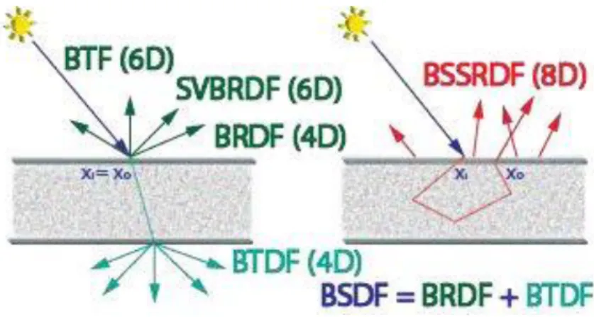
Figure 1.1 The details of the material-light interaction. When the light’s entry and outgoing points are the same, BSDF, SVBRDF or BRDF may be used in the simulation. If the entry point is different than the outgoing point, BSSRDF should be used for the
simulation (Kurt, 2014) 1
Figure 1.2 Rendering sample of orange juice (Donner et al., 2009) 2
Figure 1.3 The output of a rendered human face. The left image is rendered using the BRDF model and the right image is rendered using the BSSRDF model. As it can be seen, the BRDF model gives unnatural, rough appearance where the BSSRDF model gives a smooth appearance (Jensen, 2001) 3
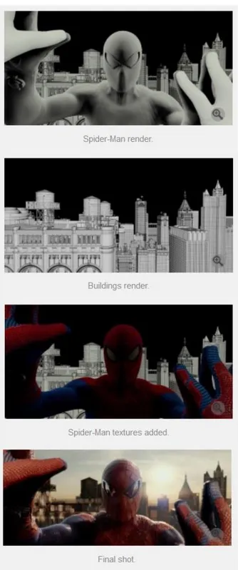
Figure 2.1 An Offline Rendering Sample in Movie Industry – The Ultimate Spiderman
Movie (Seymour, 2012) 5
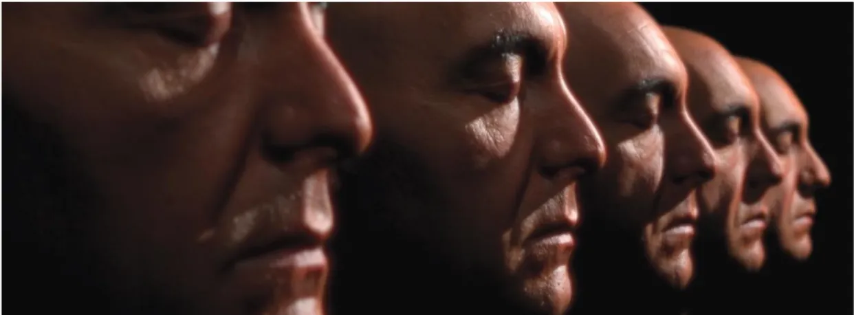
Figure 2.2 A real-time rendering sample of multiple human faces in one scene that performs subsurface scattering (Jimenez et al., 2009) 6
Figure 2.3 Scanline Rendering example that uses triangle as the primitive. The pixels affected by the projection is shown (Kleiman, 2012) 7
Figure 2.4 The demonstration of Ray Tracing technique that shows the rays traced from
the view point. (Cutler, 2008) 8
Figure 2.5 The final image with ray tracing technique that uses direct illumination (upper), the radiosity effect is shown that also uses secondary illumination sources that reflects from the surfaces (lower) (Kinkelin et al, 2008) 9
Figure 2.6 The demonstration of path tracing technique. In path tracing technique, only one secondary ray is traced which is chosen randomly. Tracing operation continues recursively similar to ray tracing (Cutler, 2008) 10
xi
Figure 2.7 The left image shows the casted rays from the light source. The right image shows the photons that are chosen with respect to the interaction points of the casted
rays (Bouatouch, 2012) 10
Figure 2.8 The left image shows the stored photons on a spatial data structure called kd-tree (shown with red) for fast access. The right image shows the k closest photons that are analyzed as an example chosen for the radiance estimation (Bouatouch, 2012)
11
Figure 3.1 Blinn’s simulation of the cloud layer over a hypothetical planet. Left image is the unclouded, randomly color squared planet. The middle image is the cloud layer and the right image is the combination of the planet surface and the cloud layer (Blinn,
1982) 13
Figure 3.2 The simulation of leaves under different lightning conditions. The left two images are backlit, the right two images are front lit (Hanrahan and Krueger, 1982) 14
Figure 3.3 The simulation of the weathering of the marble statue of Diana the Huntress. Erosion and yellowing effects has been handled accurately in their work (Dorsey et al.,
1999) 15
Figure 3.4 The rendered images of translucent teapot. The left image is rendered by a sampled BSSRDF, and the right image is rendered by Jensen and Buhler’s model. The images have similar quality; however, sampled BSSRDF renders the teapot in 18 minutes where Jensen and Buhler’s model renders in 7 seconds (Jensen and Buhler,
2002) 17
Figure 3.5 The output of Mertens et al.’s study of human skin. It is not an applicable solution for heterogeneous translucent materials (Mertens et al., 2005) 17
Figure 3.6 The work of Tong et al.’s on a sponge material. The left image is rendered from a captured material model, the right image is the actual photograph (Tong et al.,
2005) 18
Figure 3.7 A factored composite wax material is applied to the Stanford dragon. The material is composed of two kinds of wax with different scattering properties. Left
xii
image is illuminated by an area light source from above and the right image is illuminated by a texture projection light from above (Peers et al., 2006) 19
Figure 3.8 SubEdit’s output. The left image is the original image. The middle image is applied bilateral filtering to the blue and white stones only. (Song et al., 2009) 20
Figure 3.9 The resulting image of the rendered material made of orange soap. The source image is given in the left corner (Munoz et al., 2011) 20
Figure 3.10 Rendered human skin. The left image is Caucasian skin, the middle image is Asian skin and the right image is African skin (Donner et al, 2006) 21
Figure 3.11 Rendered human skin. Left image is with no subsurface scattering where the model completes the effect in good accuracy (Jimenez et al., 2010a) 22
Figure 3.12 Output of Jimenez et al.’s work which demonstrates different states of human face in manners of physical and psychological terms (Jimenez et al., 2010b) 23
Figure 4.1 The illustration of acquiring 𝑅𝑑′ from 𝑅𝑑 (Kurt et al., 2013) 25 Figure 4.2 The illustration of acquiring G matrix and the final matrix to be used for factorization operation. Left image is G matrix and the right image is the division
operation (Kurt, 2014) 26
Figure 4.3 The illustration of clustering operation on materials with more than one heterogeneous structure (Kurt, 2014) 26
Figure 4.4 (a) The diffuse BSSRDF matrix (b) The substitution operation that is done on 𝑅𝑑 to get 𝑅𝑑′ (c) Shifting operation to get 𝑅𝑑′′ (Kurt, 2014) 28 Figure 4.5 The illustration of error modelling approach on Tucker factorization (Kurt,
2014) 28
Figure 4.6 The Tucker-based factorization model has two parameters; P and T. T is the number of terms and P is the order of the polynomial in the factorization operation. For different values of T and P, RMSE values are achieved (Kurt, 2014) 29
xiii
Figure 4.7 The illustration of error modelling approach on SVD (Kurt, 2014) 31
Figure 4.8 The SVD-based factorization model has one parameter; S. S is the number of terms in the factorization operation. For different values of S, RMSE values are achieved and the compression rate is shown (Kurt, 2014) 31
Figure 5.1 The graphical user interface of our integration plugin in the Blender 3D Modeling Tool (Blender Foundation, 2003) 37
Figure 5.2 A general overview of Blender 3D Modeling Tool (Blender Foundation,
2003) and our integration plugin 38
Figure 5.3 A general overview of Blender rendering page (Blender Foundation, 2003) that connects to Mitsuba Renderer’s GUI (Jakob, 2010) through our integration plugin
39
Figure 6.1 A preview scene of our integration plugin in the Blender 3D Modeling Tool using chessboard (4 x 4) representation 40
Figure 6.2 A dragon under spot lighting was rendered using our integration plugin using
chessboard (4 x 4) 41
Figure 6.3 A dragon under spot lighting was rendered using our integration plugin using
chessboard (8 x 8) 41
Figure 6.4 A kitten under spot lighting was rendered using our integration plugin using
chessboard (4 x 4) 42
Figure 6.5 A kitten under spot lighting was rendered using our integration plugin using
xiv
INDEX OF TABLES
Table 4.1 Details of the material types that Peers et al. measured. Two main material types have been used in the representation of heterogeneous translucent materials (Kurt, 2014) ... 24
xv
INDEX OF SYMBOLS AND ABBREVIATIONS Abbreviations
ALS Alternating Least Squares
BRDF Bidirectional Reflectance Distribution Function
BSDF Bidirectional Scattering Distribution Function
BSSRDF Bidirectional Scattering Surface Reflectance Distribution Function
BTDF Bidirectional Transmittance Distribution Function
BTF Bidirectional Texture Function
CR Compression Ratio
GUI Graphical User Interface
NMF Non-Negative Matrix Factorization
RMSE Root-Mean-Square Error
RTE Radiative Transfer Equation
SSS Subsurface Scattering
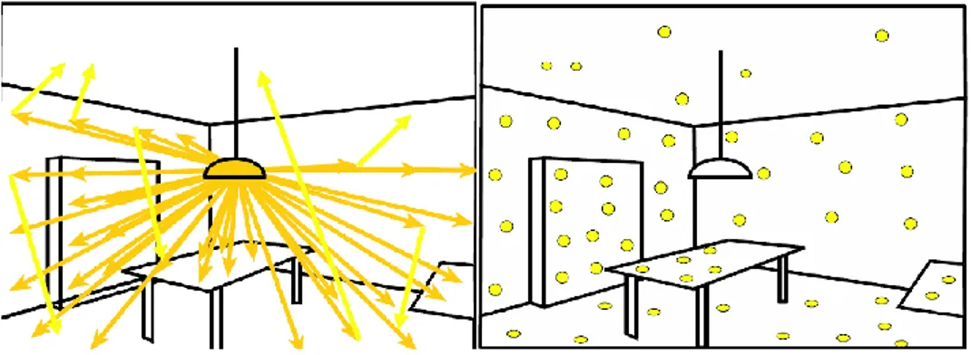
1 1 INTRODUCTION
In rendering operations, the aim is getting more realistic images. The advanced rendering techniques and features help to achieve this aim; however, the representation of the material is also an important factor in the realistic visualization of the scene. Different types of functions are used to represent different types of materials. This is the result of the fact that the light is transported following different paths related to the characteristics of the material. For example; for opaque materials, the best effect is achieved by using Bidirectional Scattering Distribution Function (BSDF). For materials similar to car paint can be simulated by using Bidirectional Reflectance Distribution Function (BRDF). There is also another function for the materials that has different amounts of reflectance at different points of their surfaces. This function is called Spatially-varying Bidirectional Reflectance Distribution Function (SVBRDF) and wooden table can be given as an example material that shows this behavior. (Kurt, 2014) If the rendering operation consist 3D textures, Bidirectional Texture Function (BTF) is the most effective function. Figure 1.1 shows the paths that the light follows corresponding to the function used for the simulation.
Figure 1.1 The details of the material-light interaction. When the light’s entry and outgoing points are the same, BSDF, SVBRDF or BRDF may be used in the simulation. If the entry point
is different than the outgoing point, BSSRDF should be used for the simulation (Kurt, 2014)
The study in this thesis is based on the behavior of the translucent materials. Translucent materials need the consideration of subsurface scattering (SSS) mechanism which defines how the light should be transported under the surface of the material. When light hits the surface of a translucent material, it scatters inside the surface and then leaves the material from another point. Such kind of effect is given by using Bidirectional Scattering Surface Reflectance Distribution Function (BSSRDF)
2
(Nicodemus et al, 1977). Some materials that are proper to be simulated by BSSRDF are marble, human skin, milk, wax, orange juice (Kurt, 2014). Figure 1.1 shows how light is transported under the surface and Figure 1.2 is a rendering sample produced by BSSRDF. Figure 1.3 shows the realistic effect of BSSRDF representation over BRDF representation on a translucent material in which the chosen material is human skin.
Figure 1.2 Rendering sample of orange juice (Donner et al., 2009)
The main subject of this thesis is the BSSRDF representation of heterogeneous translucent materials. In consequence of the investigations in the literature, Singular Value Decomposition (SVD) method is analyzed as more accurate and efficient with respect to other existing methods. It is implemented in C++ and imported into the Mitsuba Renderer project (Jakob, 2010). The final outcome of this thesis is a renderer plugin that works efficiently and accurately on Blender 3D modelling tool (Blender Foundation, 2003). The plugin is verified by using a set of measured heterogeneous subsurface scattering data sets which will be detailed in the section six.
3
In this thesis, section two discusses the rendering process with the details of its classifications and techniques. Section three refers the previous work based on subsurface scattering. This part is divided into two subsections: the first part explains the properties of BSSRDF, the second part introduces subsurface scattering models. This subsection is also divided into three parts. The first part mentions the analytical subsurface scattering models, the second part introduces the data-driven subsurface scattering models and the last part refers the multi-layered subsurface scattering models. Section four explains the preparation of the test data for the representation of heterogeneous translucent materials and also two factorization algorithms that can use these data to achieve subsurface scattering. Section five discusses Blender 3D Modelling tool and Mitsuba Renderer which are the software that the plugin is integrated with and how the plugin is developed. In section six, the plugin’s experimental results are shown and the performance details are discussed. Section seven is conclusion and the section eight is the last part in this thesis which consist the discussions of possible improvements and other software modelling platforms that the plugin can be integrated with.
Figure 1.3 The output of a rendered human face. The left image is rendered using the BRDF model and the right image is rendered using the BSSRDF model. As it can be seen, the BRDF model gives unnatural, rough appearance where the BSSRDF model gives a smooth appearance
4 2 RENDERING
The study in this thesis is based on getting the most realistic subsurface scattering effects on heterogeneous translucent materials through the usage of Mitsuba renderer (Jakob, 2010) and Blender 3D modelling tool (Blender Foundation, 2003). Therefore, this section explains the essential process of the study which is the rendering operation by detailing its types and techniques.
2.1 Description of Rendering
Rendering is the process of creating 2D images from models that are created with 3D modelling tools. It is an important step in graphical representation since the final appearance of the model is given by this process. In the areas of architecture, video games, simulators, movies and design visualization we can see several examples of rendering samples. Rendering process can be classified into two sections: offline rendering and real time rendering (Thadani, 2000).
Offline Rendering
Offline rendering is the method that is not done in real time which also means that the scenes are rendered before the product is complete and combined with other elements to create the environment of the product. As an example, animations of the video games can be given. The developers of the game, render several scenes during the production and combine them together to create the animations in the video games. This method offers the usability of much more powerful and complex models which increases the visualization quality rather than real time rendering offers. However, the weakness of this approach is the inability to modify the details of the offline rendered scenes (especially a weakness for the game industry where interactivity with the environment is needed) and the approach is slower than real time rendering. We can see offline rendered 3D graphics scenes in the game industry where we can give the examples of the first two games of Age of Empires series and most games of Resident Evil series. The movie industry also widely uses offline rendering. Figure 2.1 shows an offline rendered scene used in movie industry.
5
Figure 2.1 An Offline Rendering Sample in Movie Industry – The Ultimate Spiderman Movie (Seymour, 2012)
6 Real Time Rendering
Real time rendering differs in many ways from offline rendering. The main difference of real time rendering from offline rendering is that the renderer uses the user’s own engine, its models and textures and GPU in order to produce the rendered scene. Thus, we can say that the user’s pc does the rendering process instead of the developer and these scenes are used in the product. This brings the advantage of much more dynamic scenes where the user can interact with the environment. However, the visualization quality is lower and when the product user has limited hardware; the performance can become a problem. Figure 2.2 is an example for real time rendering approach with sunlight illumination.
Figure 2.2 A real-time rendering sample of multiple human faces in one scene that performs subsurface scattering (Jimenez et al., 2009)
2.2 Rendering Techniques
Rendering process analyze the details of spatial, textural, color and lighting information in the scene. (Slick, 2014) These details are combined and then the final image is evaluated. The evaluation process can differ with respect to the view-point of the renderer. (Thadani, 2000) Although there are many rendering techniques, five major techniques are widely used for the evaluation process currently. These techniques vary in the calculation of the sample scene’s rendering information. Other rendering features (caustics, shading, texture mapping, translucency, soft shadowing, motion blur, and others) can be added into the rendering process to get powerful effects and increase the realism of the scene.
7 Scanline Rendering
Scanline rendering is the approach of using triangles and polygons instead of pixels as the primitives of the rendering process. A primitive-by-primitive approach is computed in this technique and the affected pixels are determined. Then, these pixels are modified according to the algorithm. (Dobbins, 2012) The illustration of the affected pixels can be seen in Figure 2.3.
Main advantage of scanline rendering is the speed of the technique. The technique does not render every pixels existing in the scene but it results in less time than the other techniques need. On the contrary, pixel-by-pixel approach results in higher quality images. (Dobbins, 2012)
Figure 2.3 Scanline Rendering example that uses triangle as the primitive. The pixels affected by the projection is shown (Kleiman, 2012)
Ray Tracing
Another major rendering technique is ray tracing. In this approach, rays are traced passing through the pixels in the scene. The algorithm continues tracing the rays until maximum number of iterations is reached (recursive) or the light source is hit or the ray leaves the scene as it is shown in Figure 2.4. (Dobbins, 2012) Then, the renderer computes the information by combining them with the intensity and color values and it paints the pixel according to the result. (Thadani, 2000)
8
The biggest advantage of this technique is the calculation of reflections and refraction of light accurately. With this ability, shadowing in the scene becomes much more effective. On the contrary, the recursive algorithm is slow and not suitable for real time rendering applications which needs to render the scene in milliseconds.
Figure 2.4 The demonstration of Ray Tracing technique that shows the rays traced from the view point. (Cutler, 2008)
Radiosity
Radiosity is the technique that secondary illumination sources are considered. Directly illuminated surfaces in the scene behave as indirect light sources and the reflected light from them illuminates other surfaces. Like the algorithm of ray tracing, this approach continues recursively until a maximum number of iterations is reached. (Dobbins, 2012)
Although the recursive algorithm is slow, the resulting image is in higher quality. The effect of shadowing the scene becomes much more realistic by the use of radiosity in the calculation of rendering (Figure 2.5 shows the effect of radiosity). There are several techniques to optimize the radiosity calculation. The reuse of radiosity for several frames can be given as an example to such optimizations.
9
Figure 2.5 The final image with ray tracing technique that uses direct illumination (upper), the radiosity effect is shown that also uses secondary illumination sources that reflects from the
surfaces (lower) (Kinkelin et al, 2008)
Path Tracing
Path tracing is a Monte Carlo rendering technique that is modified from conventional ray casting technique. The method differs from ray casting in its light sampling method in which a set of ray paths are traced from the view point to the light source similar to ray casting, however, only one secondary ray per recursion is traced to calculate the indirect illumination (Cutler, 2008). The recursion continues until all primary rays are traced according to the algorithm.
10
Figure 2.6 The demonstration of path tracing technique. In path tracing technique, only one secondary ray is traced which is chosen randomly. Tracing operation continues recursively
similar to ray tracing (Cutler, 2008)
Photon Mapping
Photon mapping technique is discovered by Jensen (1996), as a practical model for subsurface scattering. It is a two pass global illumination technique; first rays are casted from light sources where photons are stored for fast access on a spatial data structure (kd tree) and then the radiance is estimated by the path of the casted ray where k closest photons are analysed (Jensen, 1996). Figure 2.7 and Figure 2.8 show the illustration of the technique.
Figure 2.7 The left image shows the casted rays from the light source. The right image shows the photons that are chosen with respect to the interaction points of the casted rays (Bouatouch,
11
Figure 2.8 The left image shows the stored photons on a spatial data structure called kd-tree (shown with red) for fast access. The right image shows the k closest photons that are analyzed
as an example chosen for the radiance estimation (Bouatouch, 2012)
Photon mapping and path tracing techniques both give accurate results for the sample inputs. As the number of samples per pixel increases, these techniques give much more efficient results. However, the techniques become very expensive for the translucent materials with high albedo (such as milk and skin). Therefore, the researches in the area of representation of translucent materials still continue which will be detailed in the following section of “Related Work”.
12 3 PREVIOUS WORK
3.1 Properties of BSSRDF
BSSRDF is the function that is used for simulating effective and accurate subsurface scattering effect. Its measurement is meter-2steradian-1 (Nicodemus et al., 1977). BSSRDF is calculated using the function below:
𝑑𝐿𝑜(𝑥𝑜, 𝜔⃗⃗ 𝑜) = 𝑆(𝑥𝑖, 𝜔⃗⃗ 𝑖; 𝑥𝑜, 𝜔⃗⃗ 𝑜)𝑑𝜑(𝑥𝑖, 𝜔⃗⃗ 𝑖) (2.1) In this equation, outgoing radiance is computed by integrating the incident radiance over incoming directions and area A (Jensen et al., 2001). The function below shows this calculation in which S denotes for the BSSRDF. BSSRDF is found to be 8D in the given formula (Kurt, 2014).
𝐿𝑜(𝑥𝑜, 𝜔⃗⃗ 𝑜) = ∫ ∫ 𝐿𝐴 Ω+ 𝑖(𝑥𝑖, 𝜔⃗⃗ 𝑖)𝑆(𝑥𝑖, 𝜔⃗⃗ 𝑖; 𝑥𝑜, 𝜔⃗⃗ 𝑜)(𝜔⃗⃗ 𝑖, 𝑛⃗ )𝑑𝜔⃗⃗ 𝑖𝑑𝑥𝑖 (2.2)
There are three main properties of BSSRDF. These are reciprocity, energy conservation and non-negativity. Reciprocity is the principle of reversibility of light transport paths and it ensures that for any visible scene point, the ratio of outgoing radiance is the same with for the incident radiance (Zickler et al., 2002). In the function this feature is shown with semicolon in BSSRDF function (S) and it means that we can change the arguments of 𝑥𝑖, 𝜔⃗⃗ 𝑖 with 𝑥0, 𝜔⃗⃗ 0 if they have the same refractive index. According to non-negativity property, a BSSRDF should take a positive value (≥0) and the property of energy conservation is formulated with the function below (Kurt, 2014):
∨ (𝑥𝑜, 𝜔⃗⃗ 𝑜), ∫ ∫ 𝑆(𝑥𝐴 Ω+ 𝑖, 𝜔⃗⃗ 𝑖; 𝑥𝑜, 𝜔⃗⃗ 𝑜)(𝜔⃗⃗ 𝑖∙ 𝑛⃗ )𝑑𝑥𝑖 ≤ 1 (2.3)
As the subsurface scattering models are modelled by using BSSRDF, simplified or not, they should also have the same properties that are valid for BSSRDF. With these properties, the subsurface scattering models can be verified to be accurate to represent translucent materials (Kurt, 2014).
The translucent materials are classified in 3 groups: homogeneous translucent materials, quasi-homogeneous translucent materials and heterogeneous translucent materials. The next subsection analyzes subsurface scattering models in three groups
13
(analytical, data-driven and multilayered) which also details the translucent material type that they are effective on.
3.2 Subsurface Scattering Models
This section introduces the previous work on the representation of translucent materials. As previously mentioned, the analysis of these studies are classified according to their approach characteristics.
Analytical Subsurface Scattering Models
The traditional approach in the area of subsurface scattering was based on the Radiative Transfer Equation (RTE) (Chandrasekhar, 1960). RTE defines radiance by considering absorption, scattering and emission in the integral form. The solution of this equation gives the effect of subsurface scattering and the equation can be solved by using Monte Carlo methods, finite element methods or photon mapping technique (Kurt, 2014).
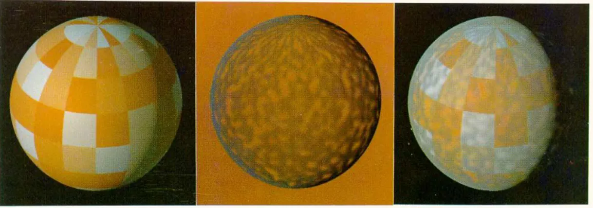
Blinn (1982) modelled the rings of Saturn using RTE in his work. He considered the rings as homogeneous translucent layers of dusty and cloudy particles (Bosch, 2007) which affect the light scattering inside the layers. This work is considered as a starting point in realistic subsurface scattering. His simulation of the cloud layer over a hypothetical planet can be seen in Figure 3.1.
Figure 3.1 Blinn’s simulation of the cloud layer over a hypothetical planet. Left image is the unclouded, randomly color squared planet. The middle image is the cloud layer and the right
14
Although the resulting images seem visually plausible, the model is built on the idea of single scattering inside the layers which is not a proper model for higher order scattering events. Another issue in this model is the outgoing radiance relation with the properties of the chosen material, and Blinn used a combination of a Lambertian and Henyey-Greenstein functions as the analytic function to model his sample of dusty and cloudy surfaces.
Kajiya (1984) extended Blinn’s model (1982) by using ray tracing to enable multiple scattering against particles with high albedo such as clouds and dust. This was an improvement since Blinn’s model was limited for the particles with low albedo. However, their approach was also based on RTE and the approach needed costly methods in order to achieve an accurate result.
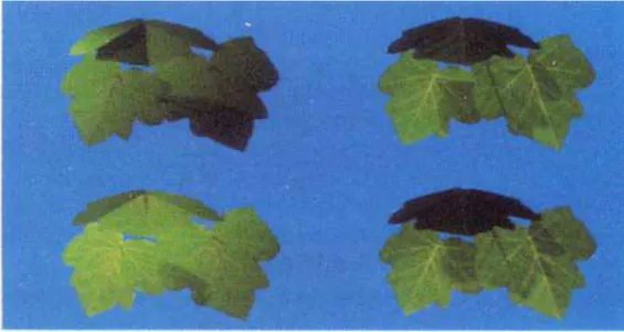
Hanrahan and Krueger (1993) proposed a similar approach to Blinn’s (1982); however, their model was based on one-dimensional linear transport theory instead of a Lambertian component. Their model is more accurate for single scattering in layered materials. Nevertheless, it is limited to uniformly lit, homogeneous slabs. They tested their model on a leaf object and they used a conventional ray tracer for their rendering process. The resulting image can be seen in Figure 3.2.
Figure 3.2 The simulation of leaves under different lightning conditions. The left two images are backlit, the right two images are front lit (Hanrahan and Krueger, 1982)
15
Dorsey et al. (1999), represented weathered stone using photon mapping technique. Using a slab data structure, they represented the deterioration process of the stone and simulated the changes in the structure of the material that is caused by the external factors. The effect of subsurface scattering is again handled by solving RTE however photon mapping technique becomes costly again for the materials with high albedo. The resulting image of their work can be seen in Figure 3.3 in which they simulated the aging process on a marble material (Diana the Huntress statue).
Figure 3.3 The simulation of the weathering of the marble statue of Diana the Huntress. Erosion and yellowing effects has been handled accurately in their work (Dorsey et al., 1999)
The previous studies mentioned in this subsection are costly and slow (Kurt, 2014). Therefore, some researchers focused on this problem and proposed another model that solves RTE faster than and as accurate as these models. This model is firstly proposed by Stam (1995) and it is called as diffusion approximation model. This model is based on the observation that the light is isotropic in highly scattering media since the light is blurred due to the scattering events. Therefore, Eq. (2.2) can be separated into a local and a global component where the local component represents the reflected light and global component represents the scattering light in material volume (Kurt et al., 2013). The global component is represented by the diffuse BSSRDF (Peers et al., 2006; Kurt et al., 2013).
16 𝑆𝑑(𝑥𝑖, 𝜔⃗⃗ 𝑖; 𝑥𝑜, 𝜔⃗⃗ 𝑜) =
1
𝜋𝐹𝑖(𝑥𝑖, 𝜔⃗⃗ 𝑖)𝑅𝑑(𝑥𝑖, 𝜔⃗⃗ 𝑜)𝐹𝑜(𝑥𝑜, 𝜔⃗⃗ 𝑜) (2.4)
Eq. (2.4) represents the diffuse BSSRDF Sd with a four dimensional (4D) spatial
subsurface scattering component Rd and the directionally dependent components Fi and Fo. The directionally dependent components are ignored and Rd is focused in the
modeling process (Peers et al., 2006; Kurt et al., 2013; Goesele et al., 2004; Song et al., 2009)
As the diffusion equation does not have an analytical solution in the case of finite media, Jensen et al. (2001) proposed a dipole (two point sources near the surface) model motivated by the researches in medical physics (Farrell et al, 1992; Eason et al., 1978) and developed a solution for the problem. Their model also enabled single scattering and a practical sampling technique for rendering which provided inspiration to other studies on the representation of translucent materials (Jensen and Buhler, 2002; Jakob et al., 2010; d’Eon and Irving, 2011).
The dipole diffusion approximation model of Jensen et al.’s (2001) is efficient and accurate on homogeneous translucent materials. Figure 1.3 is an example of this model’s superiority over the BRDF model which was used commonly in previous studies. However, the model is not efficient on heterogeneous translucent materials due to the observation that relies behind the theory which is the material having a high albedo (Donner, 2006). As the albedo decreases, the light is absorbed inside the surface of the material and it cannot diffuse far away (Donner, 2006).
Jensen and Buhler (2002) proposed a two pass rendering technique. In the first pass, sample points are stored on the surface and irradiance is computed according to these sample points. In the second pass, a hierarchical evaluation technique is used that used dipole diffusion approximation model that computes radiant exitance. The model is faster than Jensen et al.’s BSSRDF (2001), however, it has a similar approach. Figure 3.4 shows the performance of their model over a sampled BSSRDF.
Mertens et al. (2005) modelled human skin using dynamic models with local subsurface scattering. They introduced an importance sampling scheme that operates in image-space. They also modified Jensen et al.’s (2001) model as an integral in image-space and combined it with importance sampling. The resulting images are not
17
highly qualified, which is a result of their subsurface scattering model. Figure 3.5 is the resulting image that they achieved for human skin.
Figure 3.4 The rendered images of translucent teapot. The left image is rendered by a sampled BSSRDF, and the right image is rendered by Jensen and Buhler’s model. The images have similar quality; however, sampled BSSRDF renders the teapot in 18 minutes where Jensen and
Buhler’s model renders in 7 seconds (Jensen and Buhler, 2002)
Jakob et al. (2010) extended the dipole diffusion approximation model by using an anisotropic approach. Although the model is capable of representing isotropic and anisotropic translucent materials, the rendered images by their approach is not visually plausible (Kurt, 2014).
Figure 3.5 The output of Mertens et al.’s study of human skin. It is not an applicable solution for heterogeneous translucent materials (Mertens et al., 2005)
18
Data-Driven Subsurface Scattering Models
A group of researchers studied measuring Rd(xi,xo) in order to enable efficient
subsurface scattering. This subsection will explain these studies.
Goesele et al. (2004) developed a compact model that depends on underlying geometry. Their measurement device was called DISCO and their aim was to analyze the behavior of dense translucent objects. The sample materials that are used in the study were nonhomogeneous objects of an alabaster horse sculpture, a rubber duck and a star fruit. The choice of the sample materials were related with the validation of the method on the materials with different behaviors. DISCO was also useful to analyze the weaknesses and strengths of the existing rendering techniques where Fuchs et al. (2005) also used it to analyze their approach.
Tong et al.’s study (2005) was based on quasi-homogeneous materials. They defined an object model based on two key observations. At a local level, the heterogeneity of a volume leads to nonhomogeneous subsurface scattering and at a larger scale; small neighborhoods on the volume have similar material composition and distribution. Therefore, the material would become a translucent material with uniformly distributed heterogeneous elements (Kurt, 2013). Their model consists 4 components: local reflectance function R(x,wi,wo), the mesostructure exitance function fv(xo,wo), mesostructure entrance function f(wi) and the global dipole term Rd(xi,,xo).
The model is effective on quasi-homogeneous materials; however, it is not a global solution to the representation of heterogeneous translucent materials. Figure 3.6 shows their work on a sponge material.
Figure 3.6 The work of Tong et al.’s on a sponge material. The left image is rendered from a captured material model, the right image is the actual photograph (Tong et al., 2005)
19
Peers et al. (2006) measured Rd(xi,xo) of heterogeneous materials in their study
(Kurt, 2014). Inspired by Tong et al.’s work (2005), Peers et al. (2006) represented a material model for the spatial component of highly heterogeneous subsurface scattering materials. The acquisition setup that they had introduced needs a compact factored form of representation for the rendering operation. They used non-negative matrix factorization in order to achieve this representation which has some advantages of positive light transport calculation and the ability to provide importance sampling. Their model is a good solution for heterogeneous translucent materials which can be seen from the resulting image in Figure 3.7.
Figure 3.7 A factored composite wax material is applied to the Stanford dragon. The material is composed of two kinds of wax with different scattering properties. Left image is illuminated by an area light source from above and the right image is illuminated by a texture projection light
from above (Peers et al., 2006)
Song et al. (2009) introduced SubEdit representation which allows interactive editing and rendering of translucent materials. This representation uses real time rendering and the method is based on decoupling non-local scattering properties into radial scattering profiles which allows real time editing on the sample materials. Their model seems to give visually plausible results which can be seen in Figure 3.8, however, Peers et al.’s model (2006) gives a more accurate result at a similar rate of compression (Kurt, 2014).
20
Figure 3.8 SubEdit’s output. The left image is the original image. The middle image is applied bilateral filtering to the blue and white stones only. (Song et al., 2009)
Munoz et al. (2011) presented a method for the approximation of the BSSRDF of homogeneous translucent objects. Their method combines a set of basis functions for the estimation of the diffuse reflectance function. Using Hermite interpolation, they also smoothed their function to reduce the noise. Their study also mentions extending the approach for the cases of uncontrolled single image environments. The approach is accurate and efficient for the representation of homogeneous translucent materials; however, the representation of heterogeneous translucent materials does not give satisfying results. As an example, Figure 3.9 can be viewed where researchers modelled some homogeneous materials such as orange soap, wax and grape. Figure 3.9 shows the resulting image of the orange soap material.
Figure 3.9 The resulting image of the rendered material made of orange soap. The source image is given in the left corner (Munoz et al., 2011)
21
Kurt et al. (2013) introduced a similar approach to Peers et al.’s (2006) with a difference of using Tucker-based factorization instead of non-negative matrix factorization (NMF). As this thesis also covers the same subject, the details of the Tucker-based factorization will be discussed in the next section.
Multilayered Subsurface Scattering Models
In this subsection, multi-layered subsurface scattering models are analyzed. The main property of the models is that they are representing the materials with multilayers such as human skin. As the results show, multi-layered models are more accurate on multi-layered materials. Some of the studies of previous subsections can also be classified here. However, they will not be explained again since they have already been detailed.
Donner and Jensen (2005) proposed a multipole diffusion approximation model. The motivation of the study was to solve the problem of scattering of light in the cases of thin translucent slabs and multilayered materials. Their results were good enough to claim that the new model works accurately, though they accepted that future work should be concentrated on objects with internal structures.
Donner and Jensen (2006) also modelled human skin by presenting a spectral shading model. The model controls the amounts of melanin, hemoglobin and oiliness and it multipole diffusion approximation model analyzes human skin in two layers (epidermis and dermis). Validation of the model is done by simulating different skin types such as Asian, African and Caucasian. The resulting images are shown in Figure 3.10.
Figure 3.10 Rendered human skin. The left image is Caucasian skin, the middle image is Asian skin and the right image is African skin (Donner et al, 2006)
22
D’Eon et al. (2007) presented a technique that approximates diffusion profiles of thin homogeneous slabs that combines Gaussian basis functions. As the technique is claimed to require no computation, the representation of human skin is accelerated. The technique uses real time rendering which is an important achievement. Nevertheless, the model has some limitations such as the probability of getting inaccurate results for highly concave objects.
Ghosh et al. (2008) presented a subsurface scattering model that consists 4 layers (Kurt, 2014). Their model combines them into one group in the rendering process which is an important difference with respect to other models presented (Kurt, 2014).
Jimenez et al. (2010a) represented human skin using a multilayered structure in their study. As a real time rendering approach, the representation is completed in an acceptable time and the resulting images are in good quality. Another important advantage of their model is the need for memory is much less. The rate of memory amount needed corresponding to other models is given as one-third (Jimenez et al., 2010a). No need for irradiance textures, only requiring shadow maps as input and less bandwidth usage makes the study as an important milestone in the representation of heterogeneous translucent materials. Figure 3.11 shows their subsurface scattering effect on human skin.
Figure 3.11 Rendered human skin. Left image is with no subsurface scattering where the model completes the effect in good accuracy (Jimenez et al., 2010a)
23
Jimenez et al. (2010b) also modelled human skin by considering psychological and physical states of human face. The effect of changing emotions (anger, fear, happiness and others) can be simulated easily in their model. Skin’s color change is predicted according to hemoglobin change according to the physical and psychological state of the human face. Figure 3.12 shows 5 different states modelled with their algorithm.
Figure 3.12 Output of Jimenez et al.’s work which demonstrates different states of human face in manners of physical and psychological terms (Jimenez et al., 2010b)
D’Eon and Irving (2011) modelled human skin using a modified model based on the dipole diffusion approximation model by quantizing Green’s diffusion function (Kurt, 2014). The model produces subsurface scattering effect in terms of Gaussian sums and they also proposed several improvements for film production rendering.
24
4 FACTORIZATION BASED SUBSURFACE SCATTERING 4.1 Preparation of the Test Data
Peers et al. (2006) acquired the data of several heterogeneous translucent materials by using a camera-laser setup. The detail of their process can be analyzed in their paper (Peers et al., 2006). Similar data is used in order to be used in the factorization process for getting the effect of subsurface scattering.
Eq. (2.2) is separated into two components: a local and a global component. In their study, Peers et al. (2006) ignored the local component and focused on the global component. Although they accepted that this an incorrect assumption, the result does not change (Kurt, 2014). This global component is used to model the diffuse BSSRDF
Sd. The global component is defined with the following equation:
𝐿𝑔(𝑥𝑜, 𝜔⃗⃗ 𝑜) = ∫ ∫ 𝐿𝐴 Ω 𝑖(𝑥𝑖, 𝜔⃗⃗ 𝑖)𝑆𝑑(𝑥𝑖, 𝜔⃗⃗ 𝑖; 𝑥𝑜, 𝜔⃗⃗ 𝑜)𝑑𝜔⃗⃗ 𝑖𝑑𝑥𝑖 (4.1)
Similar to Peers et al.’s (2006) work, 4D Rd(xi,xo) is measured where directional
properties are ignored (Fi, Fo). Table 4.1 shows the details of two main material types
that are modelled in this thesis (Kurt, 2014).
Table 4.1Details of the material types that Peers et al. measured. Two main material types have been used in the representation of heterogeneous translucent materials (Kurt, 2014)
Sample Material
Physical Size (cm2) Resolution
(pixels)
Core Size (pixels)
Chessboard (4x4) 12.6 x 12.6 277 x 277 39 x 39 Chessboard (8x8) 25.1 x 25.1 222 x 222 39 x 39
25
Peers et al. (2006) used factorization operation to make the data to use less memory space in the rendering process. This is the main motivation of this thesis study. However, preprocess should be done on the test data in order to make it proper for the factorization process. This operation is carried out by considering the core sizes of the heterogeneous translucent materials. For every (𝑥𝑖, 𝑥𝑜) points, the value of (xo, yo) is
taken into consideration where other values are assumed as zero (Kurt, 2014). Another important action is to perform linear regression on (𝑥𝑖, 𝑦𝑖) and (𝑥𝑖, 𝑦𝑜). After these operations, 2D 𝑅𝑑(𝑥𝑖, 𝑥𝑜) subsurface scattering data is acquired which will be used in the factorization operation.
Rd (xi, xo) is transformed into 𝑅𝑑′(𝑥𝑖, 𝑑) by using the substitution of d = xo – xi
(Peers et al., 2006; Kurt et al., 2013). Then a 𝑔(𝑑) function is calculated by averaging every column of 𝑅𝑑′ matrix. 𝐺(𝑥𝑖, 𝑥𝑜) can be found using that 𝑔(𝑑) function which is shown below (Kurt, 2014):
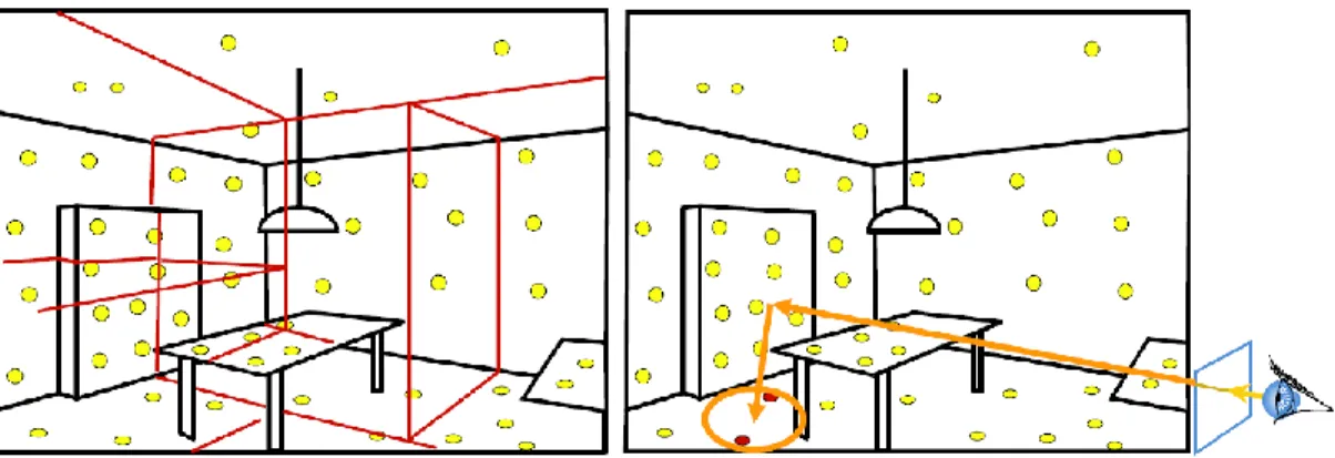
𝐺(𝑥𝑖, 𝑥𝑜) = 𝑔(𝑑) = 𝑔(𝑥𝑜, 𝑥𝑖) (4.2) After that operation, 𝑅𝑑(𝑥𝑖, 𝑑) is divided by 𝐺(𝑥𝑖, 𝑥𝑜) where the diagonal subsurface scattering properties has been acquired (Kurt, 2014). This matrix is used for the factorization operation which brings us to the model that uses less memory space for subsurface scattering effects. The illustration of these operations can be viewed from Figure 4.1 and 4.2.
26
Figure 4.2 The illustration of acquiring G matrix and the final matrix to be used for factorization operation. Left image is G matrix and the right image is the division operation
(Kurt, 2014)
Peers et al. (2006) also proposed using k-means clustering algorithm for the materials that consists more than one heterogeneous structure. However, this algorithm works slower although it increases accuracy of the model on composite structures. Kurt (2014) illustrated this clustering operation with the following figure in his Ph.D. dissertation (Figure 4.3).
Figure 4.3 The illustration of clustering operation on materials with more than one heterogeneous structure (Kurt, 2014)
27
The next subsections of this thesis explain the factorization methods that are used on the test data. Two factorization methods are analyzed with details, and they are compared with respect to their performance analysis.
4.2 Tucker-Based Factorization
Subsurface scattering data is processed as a tensor. Therefore, it is important to understand the tensor decomposition methods. Tensors are multidimensional series (Kurt, 2014). As Kolda and Bader (2009) explain, they are represented with the product of N vector spaces. They can be classified into three groups as Kurt (2014) suggests: a first order tensor which is a vector, a second order tensor which is a matrix and a higher order tensor with three or more dimensions.
There are several tensor decomposition methods; however, this thesis is focused on two methods: Tucker-based factorization and Singular Value Decomposition methods. This subsection will analyze Tucker factorization.
The reason of choosing Tucker and SVD methods are due to the fact that these factorization techniques need less space and the computation cost is not as high as other methods. The output of the rendering process also becomes more accurate with these methods (Kurt, 2014).
Tucker method takes tensors into consideration as multidimensional series. They are represented as two dimensional matrices and a core tensor that defines the relationship between them. The decomposition algorithm is the Alternating Least Squares (ALS) which is used to get the matrices and the core tensor. The details of the ALS algorithm can be examined in Kurt’s (2014) work.
There is one additional operation that is done on the test data to increase the efficiency of the model. As it is explained, 𝑅𝑑′ matrix is found from 𝑅𝑑 by using the substitution d = xo – xi. This matrix is analyzed to be the most compact data that is used
to achieve subsurface scattering. However, the Tucker-based factorization’s efficiency can be improved by the method that is proposed by Xu et al. (2011). This additional operation is getting the maximum value of each xi row and it is shifted as the maximum
value becomes the first element of that row. Then, each xi row is divided to that row’s
28
similar values to the same columns and preventing any peak values that can result because of the acquisition process (Kurt, 2014). Figure 4.4 is the illustration of that process.
Figure 4.4 (a) The diffuse BSSRDF matrix (b) The substitution operation that is done on 𝑹𝒅 to
get 𝑹𝒅′ (c) Shifting operation to get 𝑹 𝒅
′′ (Kurt, 2014)
The error modelling approach is applied on 𝑅𝑑′′ matrix (Kurt, 2013) using Tucker-based factorization for each color channel. After the first operation, two vectors are found 𝑓1(𝑥𝑖) and ℎ1(𝑑) (Kurt, 2013). Then, these model errors are factorized again for
a predetermined number of times and the final subsurface scattering model is calculated by summing the estimation of model errors and the first factorization of 𝑅𝑑′′ matrix. Figure 4.5 shows the illustration of this process. For more details, Kurt’s (2014) work can be examined.
29
Kurt (2014) explained that scattering on each color channel are similar. As the factorization is applied on averaged subsurface scattering values that are mentioned before, the prediction of deviations are modelled with a polynomial of order P. By applying linear coefficients on each xi row of the matrix, we get subsurface scattering
models for each color channel with the following equations (Kurt, 2014):
𝑅𝑑𝑟(𝑥𝑖, 𝑥𝑜) ≈ ∑ 𝛽𝑟𝑝𝑥𝑖𝑅𝑑 ′ 𝑃 𝑝=0 (𝑥𝑖, 𝑑)𝑝 𝑅𝑑𝑔(𝑥𝑖, 𝑥𝑜) ≈ ∑ 𝛽𝑔𝑝𝑥𝑖𝑅𝑑 ′ 𝑃 𝑝=0 (𝑥𝑖, 𝑑)𝑝 𝑅𝑑𝑏(𝑥𝑖, 𝑥𝑜) ≈ ∑ 𝛽𝑏𝑝𝑥𝑖𝑅𝑑 ′ 𝑃 𝑝=0 (𝑥𝑖, 𝑑)𝑝 (4.3)
Lastly, the parameter analysis shows that when the first ten terms are used, Tucker-based factorization model gives accurate results (Kurt, 2014). Figure 4.6 shows that result:
Figure 4.6 The Tucker-based factorization model has two parameters; P and T. T is the number of terms and P is the order of the polynomial in the factorization operation. For different values
of T and P, RMSE values are achieved (Kurt, 2014)
4.3 SVD Factorization
SVD method is another factorization technique that is analyzed in this thesis. The approach is applied on the similar test data (𝑅𝑑′), and following its rules the subsurface scattering model can be achieved at the end of the process.
30
In SVD operation, an M x N matrix is defined as the product of a U matrix with dimensions M x K and a matrix V with dimensions K x N and a core tensor with dimensions K x K. This is a similar decomposition operation in Kurt et al.’s (2013) study, however, if the value of K is chosen to be 1 that is a scalar then the dimensions of U and V matrices become M x 1 and 1 x N, respectively, the core tensor becomes scalar (Kurt, 2014).
In this operation, 𝑅𝑑′ is taken into consideration as it is the most compact data similar to the operation in Tucker-based factorization. Another consideration in the factorization operation is making the data stay in the positive values which leads to physically correct results. This is achieved with another transformation that is (Kurt, 2014):
𝑅𝑑′′′(𝑥𝑖, 𝑑) = ln(
𝑅𝑑′(𝑥𝑖,𝑑)
𝐴 + 𝐵) (4.4)
By choosing the most appropriate values for A and B to minimize error values, 𝑅𝑑′′′ matrix is factorized using SVD and error terms for each color channel is modelled similar to the work has been done in previous subsection. This procedure is repeated S times to improve the accuracy of the approximation (Figure 4.7). Accordingly 𝑅𝑑′′′ becomes (Kurt, 2014):
𝑅𝑑′′′(𝑥𝑖, 𝑑) ≈ ∑𝑆𝑗=1𝑓𝑗(𝑥𝑖)ℎ𝑗(𝑑) (4.5)
In the rendering process, interpolation is needed between the values of subsurface scattering. This is the reason of the stored vectors’ algorithm is piecewise lineer functions (Kurt, 2014). In the calculation of interpolation, bilinear interpolation is used between the d values of ℎ𝑗(𝑑) vector. Then the subsurface scattering model for each color channel becomes (Kurt, 2014):
𝑅𝑑𝑟(𝑥𝑖, 𝑥𝑜) ≈ 𝐴 ∗ exp(𝑅𝑑𝑟′′′(𝑥
𝑖, 𝑑)) − 𝐴 ∗ 𝐵
𝑅𝑑𝑔(𝑥𝑖, 𝑥𝑜) ≈ 𝐴 ∗ exp (𝑅𝑑𝑔′′′(𝑥
𝑖, 𝑑)) − 𝐴 ∗ 𝐵
31
Figure 4.7 The illustration of error modelling approach on SVD (Kurt, 2014)
SVD-based subsurface scattering gives convincing results for representing heterogeneous translucent materials. The work of Kurt (2014) also emphasizes that approximation results are visually acceptable for some test materials even for a small number of iteration (S≤5). This statement is also verified in this thesis as an important advantage of SVD-based subsurface scattering. Furthermore, the S value should be chosen carefully since the factorization is applied separately to each channel and the compression rate can be a problem for obtaining close approximations. The effect of number of iterations on the model errors for different materials and the compression rates via number of S is shown in Figure 4.8.
Figure 4.8 The SVD-based factorization model has one parameter; S. S is the number of terms in the factorization operation. For different values of S, RMSE values are achieved and the
32
As the results show, both factorization techniques offer accurate and efficient results. In this thesis, SVD factorization is chosen as the algorithm to be used in the representation of subsurface scattering on heterogeneous translucent materials. This choice relies on one main difference between Tucker factorization and SVD factorization. That difference is the efficiency on two dimensional matrices.
SVD approach works more efficient on two dimensional matrices. On the other hand, Tucker factorization’s efficiency increases on higher order tensors (Kurt, 2014). As the main motivation of this thesis is to increase the efficiency of heterogeneous translucent materials representation as well as to keep the level of realism, SVD fits to this thesis’ aim much better. As SVD approach’s final images are visually plausible which will be detailed in following section, this choice seems to be correct and logical.
33 5 THE INTEGRATION PLUGIN
Constructing images through modeling and representing the BSSRDF for heterogeneous translucent materials is a complicated procedure. Developing a plugin to support the heterogeneous subsurface scattering effects of the underlying materials will provide a useful tool for many applications. In this work, we aim to develop a plugin for rendering purposes. Such a plugin must be an interface between the renderer and the software modeling tool. The renderer which has the capability to represent the heterogeneous translucent materials is not the only task to be carried out. Details of lighting information, shading, texture mapping and others in the scene are defined by the 3D modeling tool and these details are also important properties that should be considered in the representation. Therefore, the plugin should send the details available on the scene to the renderer, and then the SVD-based subsurface scattering representation can be a solution for the common problem.
The procedure for developing the plugin has two steps: the first step consists of the implementation of SVD-based subsurface scattering representation in the renderer, and the second step is to create a script that is able to send the details in the scene to the SVD-based subsurface scattering representation for a visually plausible rendering.
The 3D modeling tools are powerful software to model the details of the scene. Light sources, materials and their details can easily be defined using these tools. Our main choice was the Blender project (Blender Foundation, 2003) which is an open source developing platform and uses Python (van Rossum, 1989) as its plugin scripting language. These features were effective in our choice since Python has the ability to call C++ functions without the need of any software. It is also effective in the sense that an open source application would be useful for the documentation and faster development.
Mitsuba renderer (Jakob, 2010) is chosen as the default renderer because it is highly optimized and it has good performance, scalability, easy usability and robustness are the other features of this renderer includes. As the project is in C++ and Blender supports Python, the implementation of the plugin could become easier. The version of the Blender used in this thesis is “2.69” which is compatible with Mitsuba version “0.5”. The source codes of these versions are modified to finalize the study in this thesis successfully.
34
The integrator class in Python script is defined as "class mitsuba_sss_svd". This class has control parameters for using different material types which are the possible parameters for the heterogeneous translucent materials. The plugin is tested on chessboard (4 x 4) and chessboard (8 x 8) heterogeneous translucent materials.
The choice of the material representation is done through the dropdown menu that can be seen in Figure 5.1. This menu has three choices: participating media, dipole subsurface and svd subsurface. Svd subsurface is the method that is offered in this thesis. The implementation is done with the code below:
class mitsuba_mat_subsurface(declarative_property_group): properties = [{
'type': 'enum', 'attr': 'type', 'name': 'Type',
'description': 'Specifes the type of Subsurface material', 'items': [
('dipole', 'Dipole Subsurface', 'dipole'), ('svd', 'Svd Subsurface', 'svd'),
('participating', 'Participating Media', 'participating'), #('homogeneous', 'Homogeneous Media', 'homogeneous'), #('heterogeneous', 'Heterogeneous Media', 'heterogeneous') ],
'default': 'dipole', 'save_in_preset': True }
def api_output(self, mts_context, mat):
sub_type = getattr(self, 'mitsuba_sss_%s' % self.type) params = sub_type.api_output(mts_context)
if self.type == 'dipole':
params.update({'id' : '%s-subsurface' % mat.name}) elif self.type == 'svd':
params.update({'id' : '%s-subsurface' % mat.name}) return params
Therefore, if the user wants to represent a heterogeneous material, then he/she must choose the svd subsurface in the dropdown menu to enable heterogeneous translucent material representation. This choice will add the subsurface scattering effect of the svd method which is defined in “class_mitsuba_sss_svd” as mentioned. The code of the svd method is implemented with the code below:
35 class mitsuba_sss_svd(declarative_property_group): ef_attach_to = ['mitsuba_mat_subsurface'] controls = [ 'material', 'useMaterialType', 'MatPreset' ] properties = [ { 'type':'enum', 'attr':'MatPreset', 'name':'Material Preset',
'description':'Choose one of the presets with their specified values', 'items': [ ('SVD_S10_Chess4x4', 'SVD_S10_Chess8x8), ], 'default':'SVD_S10_Chess4x4 ', 'save_in_preset': True }
def api_output(self, mts_context): params = {
'type' : 'svd' }
params.update({'material' : self.material}) return params
With this code, the user can add the subsurface scattering representation through a dropdown menu or just typing the name of the file to be used on heterogeneous materials. If he/she chooses to use the dropdown menu, two data files are offered for the representation (svd_S10_Chess4x4 or SVD_S10_Chess8x8). These details of these files are mentioned in Table 4.1. By choosing one of these sample material types, the user can create the subsurface scattering effect on heterogeneous translucent materials. The sample rendering outputs are shown in Figures 6.2, 6.3, 6.4 and 6.5 using dragon and kitten sample objects in the next section.
The integration plugin renders the material according to the material type choice and sends the data to the Mitsuba renderer .exe file, which consists of the necessary operations. These parameters are updated a function called "params.update" which is defined in the Python script. The data is kept on the object of the material chosen, by using the default constructor self of Python language.