GRADUATE SCHOOL OF SCIENCE AND ENGINEERING
COMPARISON AND ANALYSIS OF VARIOUS INDOOR POSITIONING
SYSTEMS TECHNIQUES
GRADUATE THESIS
DERYA DEMİRKOL
DERYA DEMİ R KO L M .S. T he si s 2016 S tudent’ s F ull Na me P h.D. (or M.S . or M.A .) The sis 20 11
COMPARISON AND ANALYSIS OF VARIOUS INDOOR POSITIONING
SYSTEMS TECHNIQUES
DERYA DEMİRKOL
Submitted to the Graduate School of Science and Engineering in partial fulfillment of the requirements for the degree of
Master of Science
in
COMPUTER ENGINEERING
KADIR HAS UNIVERSITY May,2016
i
ABSTRACT
COMPARISON AND ANALYSIS OF VARIOUS INDOOR POSITIONING
SYSTEMS TECHNIQUES
DERYA DEMİRKOL
Master of Science in Computer Engineering Advisor: Asst. Prof. Dr. Tamer DAĞ Co-Advisor: Asst. Prof. Dr. Taner ARSAN
May,2016
Indoor Positioning has been a research subject in order to facilitate people life easier. Different type of methods has been implemented and tested by the years. The Global Positioning System (GPS) is a satellite based navigation system. This technique is using outdoor environment to navigate people or buildings. In indoor positioning, GPS signals are usually too weak to provide accurate positioning estimate. Other technique need to investigate to get better result of accuracy. Ultrasonic Positioning Systems, RFID, Computer Vision System, RF, Wireless Indoor Positioning System has been used. Recent year, Wireless Indoor Positioning Technique is most popular technique. It is easier to set up every indoor environment by using Access Points (AP) and costs are very low comparing to other techniques. Also Wireless technique does not need any extra component or effort.
In this thesis, Indoor Positioning techniques were investigated. Different algorithms were implemented to estimate location in indoor areas and accuracy comparison has been made by using Wireless technology.
Keywords: Indoor Positioning Systems, Triangulation, Maximum Likelihood, Fuzzy Logic, Localization
AP PE ND IX C
ii
ÖZET
ÇEŞİTLİ KAPALI MEKAN KONUMLANDIRMA SİSTEM TEKNİKLERİNİN ANALİZİ VE KARŞILAŞTIRILMASI
DERYA DEMİRKOL
Bilgisayar Mühendisliği, Yüksek Lisans Danışman: Yard. Doç. Dr. Tamer DAĞ Eş Danışman : Yard. Doç. Dr. Taner ARSAN
Mayıs,2016
Kapalı mekan konumlandırma sistemleri, insanların hayatını kolaylaştırmak için araştırma konusu olmuştur. Seneler içinde ,çeşitli methodlar uygulanmış ve test edilmiştir.
Kürsel Konumlandırma Sistemi (KKS) uydu konumlandırması kullanılarak gerçekleştirilen navigasyon tekniğidir. Bu teknik dış mekanlarda insanların veya binaların konumlarının bulunmasında kullanılmaktadır. İç mekan
konumlandırılmasında KSS sinyalleri çok zayıf kaldığından doğru konumlandırma yapamamaktadır. Kullanılan diğer teknikler üzerinde çalışmalar yaparak daha doğru konumlandırma tahmini yapılmaya çalışmaktadır. Ultrasonik
Konumlandırma Sistemleri, RFID, Bilgisayar Görsellik Sistemi, RF, Kablosuz Kapalı Konumlandırma Sistemleri kullanılmıştır.
Son yıllarda Kablosuz Kapalı Konumlamdırma Tekniği en popüler tekniklerden biri olmuştır. Her türlü kapalı ortama modem kullanılarak kolaylıkla
kurulabilmesi, onu diğer tekniklerden daha az masraflı olmasını sağlamıştır. Ayrıca bu teknik sinyal kullanarak ileştişim sağladığından fazladan bileşen veya çabaya gerek duymamaktadır.
Bu tezde, Kapalı Konumlandırma teknikleri araştırlmıştır. Farklı algoritmalar uygulanarak kapalı ortamlarda konum tahmini yapılmaya çalışılmış ve bu algoritmalar arasında hassasiyet karşılaştırılması yapılmıştır.
Anahtar Kelimeler: Kapalı Konumlandırma Sistemleri, Üçgenleme, Maksimum Olabilirlik, Bulanık Mantık, Konumlandırma
AP PE ND IX C
iii
Acknowledgements
Foremost, I indebted to thank my supervisor, Asst. Prof. Tamer Dağ and Asst. Prof.
Taner Arsan, for the continuous support of my M.S. study and research, for their patience, motivation, enthusiasm, expertise and immense knowledge.
Finally, I am grateful to my family and all friends who supported me both during my studies and in writing my thesis. This journey would not have been possible without them. AP PE ND IX C
iv Table of Contents Abstract i Özet ii Acknowledgements iii List of Tables x List of Figures xi
List of Abbreviations xvi
1 Introduction 1
1.1 Background and Motivation……… 1
1.2 Existing Positioning Systems………... 4
1.2.1 Infrared Positioning Systems……… 4
1.2.2 Ultrasonic Positioning Systems……… 4
1.2.2.1 Active Bats……….. 4
1.2.2.2 Crickets……… 5
1.2.3 RSSI Positioning Systems……… 6
1.2.3.1 Radio Frequency Identification…………... ….. 6
1.2.3.2 Ultra Wide Band (UWB) Technology………… 6
1.2.3.3 RADAR Technology………... 7
1.2.3.4 Wi-Fi Technology……… 7
1.3 Position Estimate Techniques………. 8
1.3.1 Received Signal Strength Indication……….. 8
1.3.2 Time of Arrival (TOA) ……….………. 9
1.3.3 Angle of Arrival (AOA) ………... 9
1.3.4 Time Difference of Arrival (TDOA) ………. 9
2 Received Signal Strength Indicator 11
2.1 Basic Mechanisms of Propagation ……….. 11
2.1.1 Reflection ………... 11
2.1.2 Diffraction……… 11
2.1.3 Scattering……… 12
2.2 RSSI Distance Relationship……….. 12
2.2.1 Free Space Path Loss Model……… 12
2.2.2 Log Distance Path Loss Model………. 13
2.2.3 Log Normal Shadowing Model……… 13 AP
PE ND IX C
v
2.3 RSSI Measurement………...… 13
3 Experimental Area 18
3.1 Synthetic Data Set……….. 18
3.2 Measurement Area with Synthetic Dataset………. 19
3.2.1 6m x 6m Measurement Area……… 19
3.2.2 12mx12m Measurement Area……….. 19
3.2.3 24mx24m Measurement Area……….. 20
3.3 Real Data Measurement……….. 21
4 Triangulation 22 4.1 Lateration………. 22 4.2 Angulations……….. 23 4.3 Test bed……… 24 4.4 Experimental Result………. ……….. 24 4.4.1 6m x 6m Measurement Area………. 24
4.4.1.1 6mx6m Area (LOS Environment)… 25 4.4.1.2 6mx6m Area (0.5 dBm Noise) …… 25 4.4.1.3 6mx6m Area (1dBm Noise)………. 26 4.4.1.4 6mx6m Area (1.5 dBm Noise)…….. 27 4.4.1.5 6mx6m Area (2 dBm Noise)……… 27 4.4.1.6 6mx6m Area (2.5 dBm Noise) …… 28 4.4.1.7 6mx6m Area (3 dBm Noise)……… 29 4.4.1.8 6mx6m Area (3.5 dBm Noise)…… 29 4.4.1.9 6mx6m Area (4 dBm Noise)……… 30 4.4.1.10 6mx6m Area (4.5 dBm Noise)…… 31 4.4.1.11 6mx6m Area (5 dBm Noise) ……… 32
4.4.1.12 Experiment with Real Data……… 32
4.4.2 12m x 12m Measurement Area………. 33
4.4.2.1 12m x 12m Area (LOS Environment)... 34
4.4.2.2 12m x 12m Area (0.5 dBm Noise)… 34 4.4.2.3 12m x 12m Area (1dBm Noise)…… 35 4.4.2.4 12m x 12m Area (1.5 dBm Noise)... 36 4.4.2.5 12m x 12m Area (2 dBm Noise)… 36 4.4.2.6 12m x 12m Area (2.5 dBm Noise)… 37 4.4.2.7 12m x 12m Area (3 dBm Noise)…… 38
vi
4.4.2.8 12m x 12m Area (3.5 dBm Noise) …… 39 4.4.2.9 12m x 12m Area (4 dBm Noise) ……… 40 4.4.2.10 12m x 12m Area (4.5 dBm Noise) …… 40 4.4.2.11 12m x 12m Area (5 dBm Noise) ……… 41 4.4.2.12 Experiment with Real Data……… 42 4.4.3 24m x 24m Measurement Area………. 42 4.4.3.1 24m x 24m Area (LOS Environment)… 43 4.4.3.2 24m x 24m Area (0.5 dBm Noise)…… 44 4.4.3.3 24m x 24m Area (1dBm Noise)……… 44 4.4.3.4 24m x 24m Area (1.5 dBm Noise)…… 45 4.4.3.5 24m x 24m Area (2 dBm Noise)………. 46 4.4.3.6 24m x 24m Area (2.5 dBm Noise) …… 46 4.4.3.7 24m x 24m Area (3 dBm Noise) ……. 47 4.4.3.8 24m x 24m Area (3.5 dBm Noise) …. 48 4.4.3.9 24m x 24m Area (4 dBm Noise) …… 48 4.4.4.10 24m x 24m Area (4.5 dBm Noise) … 49 4.4.4.11 24m x 24m Area (5 dBm Noise) … 50 4.4.4 Experiment Results Summary Table……… 51
5 Maximum Likelihood 52
5.1 Test bed……… 54
5.2 Experimental Result………... 54 5.2.1 6m x 6m Measurement Area………. 54 5.2.1.1 6mx6m Area (LOS Environment)…… 55 5.2.1.2 6mx6m Area (0.5 dBm Noise)………. 56 5.2.1.3 6mx6m Area (1dBm Noise)………… 56 5.2.1.4 6mx6m Area (1.5 dBm Noise)……… 57 5.2.1.5 6mx6m Area (2 dBm Noise)………… 58 5.2.1.6 6mx6m Area (2.5 dBm Noise)……… 58 5.2.1.7 6mx6m Area (3 dBm Noise)………. 59 5.2.1.8 6mx6m Area (3.5 dBm Noise)…….. 60 5.2.1.9 6mx6m Area (4 dBm Noise)……… 60 5.2.1.10 6mx6m Area (4.5 dBm Noise)………. 61 5.2.1.11 6mx6m Area (5 dBm Noise) ………. 62 5.2.1.12 Experiment with Real Data……….… 63
vii
5.2.2 12m x 12m Measurement Area……… 64
5.2.2.1 12m x 12m Area (LOS Environment)…. 64 5.2.2.2 12m x 12m Area (0.5 dBm Noise)…… 65 5.2.2.3 12m x 12m Area (1dBm Noise) ……… 66 5.2.2.4 12m x 12m Area (1.5 dBm Noise) …… 66 5.2.2.5 12m x 12m Area (2 dBm Noise) ……… 68 5.2.2.6 12m x 12m Area (2.5 dBm Noise) …… 68 5.2.2.7 12m x 12m Area (3 dBm Noise) ……… 69 5.2.2.8 12m x 12m Area (3.5 dBm Noise) …… 70 5.2.2.9 12m x 12m Area (4 dBm Noise) ……… 71 5.2.2.10 12m x 12m Area (4.5 dBm Noise)……… 71 5.2.2.11 12m x 12m Area (5 dBm Noise) ……….. 72
5.2.2.12 Experiment with Real Data ……….…… 73
5.2.3 24m x 24m Measurement Area……… 73
5.2.3.1 24m x 24m Area (LOS Environment) ….. 74
5.2.3.2 24m x 24m Area (0.5 dBm Noise)………. 75 5.2.3.3 24m x 24m Area (1dBm Noise)………… 75 5.2.3.4 24m x 24m Area (1.5 dBm Noise)………. 76 5.2.3.5 24m x 24m Area (2 dBm Noise)………… 77 5.2.3.6 24m x 24m Area (2.5 dBm Noise)……… 78 5.2.3.7 24m x 24m Area (3 dBm Noise)……….. 78 5.2.3.8 24m x 24m Area (3.5 dBm Noise) …….. 79 5.2.3.9 24m x 24m Area (4 dBm Noise) ………. 80 5.2.3.10 24m x 24m Area (4.5 dBm Noise) ……. 80 5.2.3.11 24m x 24m Area (5 dBm Noise) ……… 81
5.3 Experiment Result Summary Table……… 82
6 Fuzzy Logic 83
6.1 Fuzzy Logic Algorithm……….…. 83
6.2 Test Bed………. 85
6.3 Experimental Results………. 85
6.3.1 6m x 6m Measurement Area………...…….. 86
6.3.1.1 6mx6m Area (LOS Environment)……. 86
6.3.1.2 6mx6m Area (0.5 dBm Noise)……… 87
viii 6.3.1.4 6mx6m Area (1.5 dBm Noise)…………. 88 6.3.1.5 6mx6m Area (2 dBm Noise)……… 89 6.3.1.6 6mx6m Area (2.5 dBm Noise)…………. 90 6.3.1.7 6mx6m Area (3 dBm Noise)……… 90 6.3.1.8 6mx6m Area (3.5 dBm Noise)…………. 91 6.3.1.9 6mx6m Area (4 dBm Noise)……… 92 6.3.1.10 6mx6m Area (4.5 dBm Noise)………… 92 6.3.1.11 6mx6m Area (5 dBm Noise)……… 93 6.3.1.12 Experiment with Real Data……….. 94 6.3.2 12m x 12m Measurement Area……… 94 6.3.2.1 12m x 12m Area (LOS Environment)….. 95 6.3.2.2 12m x 12m Area (0.5 dBm Noise)……… 95 6.3.2.3 12m x 12m Area (1dBm Noise)………… 96 6.3.2.4 12m x 12m Area (1.5 dBm Noise)……… 97 6.3.2.5 12m x 12m Area (2 dBm Noise)……….. 97 6.3.2.6 12m x 12m Area (2.5 dBm Noise)…….. 98 6.3.2.7 12m x 12m Area (3 dBm Noise)………. 99 6.3.2.8 12m x 12m Area (3.5 dBm Noise)…….. 99 6.3.2.9 12m x 12m Area (4 dBm Noise)………. 100 6.3.2.10 12m x 12m Area (4.5 dBm Noise)…….. 101 6.3.2.11 12m x 12m Area (5 dBm Noise)………. 101 6.3.2.12 Experiment with Real Data………. 102 6.3.3 24m x 24m Measurement Area……… 103 6.3.3.1 24m x 24m Area (LOS Environment)….. 103 6.3.3.2 24m x 24m Area (0.5 dBm Noise)……… 104 6.3.3.3 24m x 24m Area (1 dBm Noise)……….. 104 6.3.3.4 24m x 24m Area (1.5 dBm Noise)…….. 105 6.3.3.5 24m x 24m Area (2 dBm Noise)………. 106 6.3.3.6 24m x 24m Area (2.5 dBm Noise)……. 106 6.3.3.7 24m x 24m Area (3 dBm Noise)……… 107 6.3.3.8 24m x 24m Area (3.5 dBm Noise)…….. 108 6.3.3.9 24m x 24m Area (4 dBm Noise)………. 108 6.3.3.10 24m x 24m Area (4.5 dBm Noise)…….. 109 6.3.3.11 24m x 24m Area (5 dBm Noise)……….. 110
ix
6.4 Experiment Results Summary Table………. 111
7 Signal Finger Print 112
7.1 Fingerprinting Algorithm with Least Square Method………… 112
7.2 Measurement Results……… 113 7.2.1 6m x 6m Measurement Area……… 113 7.2.1.1 6mx6m Area (1 dBm Noise) ….…... 114 7.2.1.2 6mx6m Area (3 dBm Noise)…………. 114 7.2.1.3 6mx6m Area (5 dBm Noise)…………. 115 7.2.2 12m x 12m Measurement Area……… 116 7.2.2.1 12mx12m Area (1 dBm Noise)……… 116 7.2.2.2 12mx12m Area (3 dBm Noise)……… 117 7.2.2.3 12mx12m Area (5 dBm Noise)……… 118 7.2.3 24m x 24m Measurement Area……….. 118 7.2.3.1 24mx24m Area (1 dBm Noise)……… 119 7.2.3.2 24mx24m Area (3 dBm Noise)……… 120 7.2.3.3 24mx24m Area (5 dBm Noise)…….. 120
7.3 Experiments Results Summary Table……….. 121
8 Comparison of IPS Algorithms 122
8.1 Comparison of Data Type………. 122
8.1.1 Data-with-no-noise……… 122
8.1.2 Data-with-noise………. 122
8.1.2.1 6mx6m Environment Comparison…… 123
8.1.2.2 12mx12m Environment Comparison…. 124 8.1.2.3 24mx24m Environment Comparison…. 125 8.2 Comparison of Access Point Usage……….. 127
8.3 Measurement Area Restriction……….. 129
8.4 General Approach………. 129
9 Conclusion 131
References 133
Curriculum Vitae 137
x
List of Tables
Table 4.1 Triangulation Experiment Result Summary Table ... 51
Table 5.1 Maximum Likelihood Experiment Results Summary Table ... 52
Table 6.1 Fuzzy Logic Experiment Results Summary Table ... 111
Table 7.1 Finger Print Experiments Result Summary Table ... 121
Table 8.1 Algorithm Performance in LOS Environment ... 122
Table 8.2 6mx6m Measurement Area Algorithm Performance ... 124
Table 8.3 12mx12m Measurement Area Algorithm Performance ... 125
Table 8.4 24mx24m Measurement Area Algorithm Performance ... 126
xi
List of Figures
Figure 1.1 Forecast of global RLTS market by value $US millions ... 1
Figure 1.2 Survey of 74 case studies of RLTS by application ... 2
Figure 1.3 IPS model in Shopping Mall ... 3
Figure 1.4 GPS Working Principle ... 3
Figure 1.5 Active Bat System ... 5
Figure 1.6 Cricket Unit Sensor ... 5
Figure 1.7 Time and Frequency of conventional radio ... 7
Figure 1.8 Time and Frequency of UWB radio ... 7
Figure 1.9 Angle of Arrival ... 9
Figure 1.10 Time Difference of Arrival ... 10
Figure 2.1 Reflections, Diffraction, and Scattering ... 12
Figure 2.2 KHU FABLAB Corridor, Measurement Area 3D Visualization 14 Figure 2.3 KHU FABLAB Corridors, Measurement Area 2D Visualization14 Figure 2.4 Access Point No1 results at experiment-1 ... 15
Figure 2.5 Access Point No2 results at experiment-1 ... 15
Figure 2.6 RSSI measurements at experiment-2 ... 16
Figure 2.7 Access Point No1 results at experiment-2 ... 16
Figure 2.8 Access Point No2 results at experiment-2 ... 17
Figure 3.1 6mx6m Measurement Area ... 19
Figure 3.2 6mx6m Measurement Area ... 20
Figure 3.3 6mx6m Measurement Area ... 20
Figure 4.1 Lateration Method ... 22
Figure 4.2 Angulations’ Method (AOA principle) ... 23
Figure 4.3 6mx6m Measurement Area – Access Point Placement ... 24
Figure 4.4 Experiment on LOS Environment (6mx6m) ... 25
Figure 4.5 Experiment on 0.5 Noise Environment (6mx6m) ... 26
Figure 4.6 Experiment on 1 Noise Environment (6mx6m) ... 26
Figure 4.7 Experiment on 1.5 Noise Environment (6mx6m) ... 27
Figure 4.8 Experiment on 2 Noise Environment (6mx6m) ... 28
Figure 4.9 Experiment on 2.5 Noise Environment (6mx6m) ... 28
xii
Figure 4.11 Experiment on 3.5 Noise Environment (6mx6m) ... 30
Figure 4.12 Experiment on 4 Noise Environment (6mx6m) ... 30
Figure 4.14 Experiment on 4.5 Noise Environment (6mx6m) – Recruitment 31 Figure 4.15 Experiments on 5 Noise Environments (6mx6m) ... 32
Figure 4.16 Experiment with Real Data (6mx6m) ... 33
Figure 4.17 12mx12m Measurement Area- Access Point Placements... 33
Figure 4.18 Experiment on LOS Environment (12mx12m) ... 34
Figure 4.19 Experiment on 0.5 dBm Environment (12mx12m) ... 35
Figure 4.20 Experiment on 1 dBm Environment (12mx12m) ... 35
Figure 4.21 Experiment on 1.5 dBm Environment (12mx12m) ... 36
Figure 4.22 Experiment on 2 dBm Environment (12mx12m) ... 37
Figure 4.23 Experiment on 2.5 dBm Environment (12mx12m) ... 37
Figure 4.24 Experiment on 3 dBm Environment (12mx12m) ... 38
Figure 4.25 Experiment on 3 dBm Environment (12mx12m)-Recruitment ... 39
Figure 4.26 Experiment on 3.5 dBm Environment (12mx12m) ... 39
Figure 4.27 Experiment on 4 dBm Environment (12mx12m) ... 40
Figure 4.28 Experiment on 4.5 dBm Environment (12mx12m) ... 41
Figure 4.29 Experiment on 5 dBm Environment (12mx12m) ... 41
Figure 4.30 Experiments with Real Data (12mx12m)... 42
Figure 4.31 24mx24m Measurement Area – Access Point Placement ... 43
Figure 4.32 Experiment on LOS Environment (24mx24m) ... 43
Figure 4.33 Experiment on 0.5 dBm Environment (24mx24m) ... 44
Figure 4.34 Experiment on 1 dBm Environment (24mx24m)………. 45
Figure 4.35 Experiment on 1.5 dBm Environment (24mx24m) ... 45
Figure 4.36 Experiment on 2 dBm Environment (24mx24m) ... 46
Figure 4.37 Experiment on 2.5 dBm Environment (24mx24m) ... 47
Figure 4.38 Experiment on 3 dBm Environment (24mx24m) ... 47
Figure 4.39 Experiment on 3.5 dBm Environment (24mx24m) ... 48
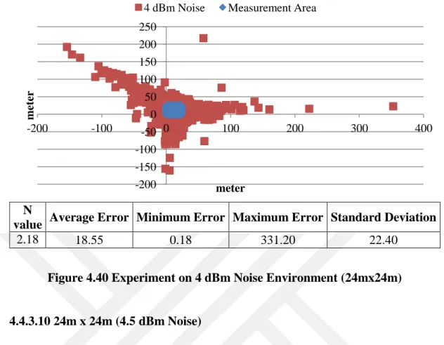
Figure 4.40 Experiment on 4 dBm Environment (24mx24m) ... 49
Figure 4.41 Experiment on 4.5 dBm Environment (24mx24m) ... 49
Figure 4.42 Experiment on 5 dBm Environment (24mx24m) ... 50
Figure 5.1 6mx6m Measurement Area – Access Point Placement ... 55
Figure 5.2 Experiment on LOS Environment (6mx6m) ... 55
xiii
Figure 5.4 Experiment on 1 Noise Environment (6mx6m) ... 57
Figure 5.5 Experiment on 1.5 Noise Environment (6mx6m) ... 57
Figure 5.6 Experiment on 2 Noise Environment (6mx6m) ... 58
Figure 5.7 Experiment on 2.5 Noise Environment (6mx6m) ... 59
Figure 5.8 Experiment on 3 Noise Environment (6mx6m) ... 59
Figure 5.9 Experiment on 3.5 Noise Environment (6mx6m) ... 60
Figure 5.10 Experiment on 4 Noise Environment (6mx6m) ... 61
Figure 5.11 Experiments on 4 Noise Environments (6mx6m) – Recruitment .. 61
Figure 5.12 Experiment on 4.5 Noise Environment (6mx6m) ... 62
Figure 5.13 Experiment on 5 Noise Environment (6mx6m) ... 63
Figure 5.14 Experiment with Real Data (6mx6m) ... 63
Figure 5.1512mxm12 Measurement Area – Access Point Placement ... 64
Figure 5.16 Experiment on LOS Environment (12mxm12) ... 65
Figure 5.17 Experiment on 0.5 Noise Environment (12mxm12) ... 65
Figure 5.18 Experiment on 1 Noise Environment (12mxm12) ... 66
Figure 5.19 Experiment on 1.5 Noise Environment (12mxm12) ... 67
Figure 5.20 Experiment on 2 Noise Environment (12mxm12) ... 68
Figure 5.21 Experiment on 2.5 Noise Environment (12mxm12) ... 68
Figure 5.22 Experiment on 3 Noise Environment (12mxm12) ... 69
Figure 5.23 Experiments on 3 Noise Environment (12mxm12) – Recruitment70 Figure 5.24 Experiment on 3.5 Noise Environment (12mxm12) ... 70
Figure 5.25 Experiment on 4 Noise Environment (12mxm12) ... 71
Figure 5.26 Experiment on 4.5 Noise Environment (12mxm12) ... 72
Figure 5.27 Experiment on 5 Noise Environment (12mxm12) ... 72
Figure 5.28 Experiments with Real Data (12mx12m) ... 73
Figure 5.29 24mx24m Measurement Area – Access Point Placement ... 74
Figure 5.30 Experiment on LOS Environment (24mx24m) ... 74
Figure 5.31 Experiment on 0.5 Noise Environment (24mx24m) ... 75
Figure 5.32 Experiment on 1 Noise Environment (24mx24m) ... 76
Figure 5.33Experiment on 1.5 Noise Environment (24mx24m)…….……... 77
Figure 5.34 Experiment on 2 Noise Environment (24mx24m) ... 77
Figure 5.35 Experiment on 2.5 Noise Environment (24mx24m) ... 78
Figure 5.36 Experiment on 3 Noise Environment (24mx24m) ... 79
xiv
Figure 5.38 Experiment on 4 Noise Environment (24mx24m) ... 80
Figure 5.39 Experiment on 4.5 Noise Environment (24mx24m) ... 81
Figure 5.40 Experiment on 5Noise Environment (24mx24m) ... 83
Figure 5.38 Experiment on 4 Noise Environment (24mx24m) ... 80
Figure 6.1 Fuzzy Logic System Design ... 83
Figure 6.2 Fuzzy Logic Membership Function ... 84
Figure 6.3 Fuzzy Logic Membership Function (continued) ... 84
Figure 6.4 6mx6m Measurement Area – Access Point Placement ... 86
Figure 6.5 Experiment on LOS Environment (6mx6m) ... 87
Figure 6.6 Experiment on 0.5 Noise Environment (6mx6m) ... 87
Figure 6.7 Experiment on 1 Noise Environment (6mx6m) ... 88
Figure 6.8 Experiment on 1.5 Noise Environment (6mx6m) ... 89
Figure 6.9 Experiment on 2 Noise Environment (6mx6m) ... 89
Figure 6.10 Experiment on 2.5 Noise Environment (6mx6m) ... 90
Figure 6.11 Experiment on 3 Noise Environment (6mx6m) ... 91
Figure 6.12 Experiment on 3.5 Noise Environment (6mx6m) ... 91
Figure 6.13 Experiment on 4 Noise Environment (6mx6m) ... 92
Figure 6.14 Experiment on 4.5 Noise Environment (6mx6m) ... 93
Figure 6.15 Experiment on 5 Noise Environment (6mx6m) ... 93
Figure 6.16 Experiment with Real Data (6mx6m) ... 94
Figure 6.17 12mxm12 Fuzzy Membership Function ... 94
Figure 6.18 Experiment on LOS Environment (12mxm12) ... 95
Figure 6.19 Experiment on 0.5 Noise Environment (12mxm12) ... 96
Figure 6.20 Experiment on 1 Noise Environment (12mxm12) ... 96
Figure 6.21 Experiment on 1.5 Noise Environment (12mxm12) ... 97
Figure 6.22 Experiment on 2 Noise Environment (12mxm12) ... 98
Figure 6.23 Experiment on 2.5 Noise Environment (12mxm12) ... 98
Figure 6.24 Experiment on 3 Noise Environment (12mxm12) ... 99
Figure 6.25 Experiment on 3.5 Noise Environment (12mxm12) ... 100
Figure 6.26 Experiment on 4 Noise Environment (12mxm12) ... 100
Figure 6.27 Experiment on 4.5 Noise Environment (12mxm12) ... 101
Figure 6.28 Experiment on 5 Noise Environment (12mxm12) ... 102
Figure 6.29 Experiments with Real Data (12mx12m) ... 102
xv
Figure 6.31 Experiment on LOS Environment (24mx24m) ... 103
Figure 6.32 Experiment on 0.5 Noise Environment (24mx24m) ... 104
Figure 6.33 Experiment on 1 Noise Environment (24mx24m) ... 105
Figure 6.34 Experiment on 1.5 Noise Environment (24mx24m) ... 105
Figure 6.35 Experiment on 2 Noise Environment (24mx24m) ... 106
Figure 6.36 Experiment on 2.5 Noise Environment (24mx24m) ... 107
Figure 6.37 Experiment on 3 Noise Environment (24mx24m) ... 107
Figure 6.38 Experiment on 3.5 Noise Environment (24mx24m) ... 108
Figure 6.39 Experiment on 4 Noise Environment (24mx24m) ... 109
Figure 6.40 Experiment on 4.5 Noise Environment (24mx24m) ... 109
Figure 6.41 Experiment on 5 Noise Environment (24mx24m) ... 110
Figure 7.1 Least Square Method Algorithm ... 113
Figure 7.2 6mx6m Measurement Area – Access Point Placement ... 113
Figure 7.3 Experiment on 1 Noise Environment (6mx6m) ... 114
Figure 7.4 Experiment on 3 Noise Environment (6mx6m) ... 115
Figure 7.5 Experiment on 5 Noise Environment (6mx6m) ... 115
Figure 7.6 12mx12m Measurement Area – Access Point Placement ... 116
Figure 7.7 Experiment on 1 Noise Environment (12mx12m) ... 117
Figure 7.8 Experiment on 3 Noise Environment (12mx12m) ... 117
Figure 7.9 Experiment on 5 Noise Environment (12mx12m)……… …..…...118
Figure 7.10 24mx24m Measurement Area – Access Point Placement ... 119
Figure 7.11 Experiment on 1 Noise Environment (24mx24m) ... 119
Figure 7.12 Experiment on 3 Noise Environment (24mx24m) ... 120
Figure 7.13 Experiment on 5 Noise Environment (24mx24m) ... 120
Figure 8.1 6mx6m Measurement Area Algorithm Performance ... 124
Figure 8.2 12mx12m Measurement Area Algorithm Performance ... 125
Figure 8.3 24mx24m Measurement Area Algorithm Performance ... 126
Figure 8.4 Comparison of Access Point Usage on 6mx6m, 12mx12m Area .... 127
Figure 8.5 Comparison of Access Point Usage on 24mx24m Area ... 128
Figure 8.6 Comparison of performance on 6mx6m, 12mx12m Area ... 129
xvi
List of Abbreviations
IPS Indoor Positioning System LBS Location Based Service PDA Personal Digital Assistant
RSSI Received Signal Strength Indication GPS Global Positioning System
LOS Line of Sight UWB Ultra Wide Band
RF Radio Frequency
WLAN Wireless Local Area Network
AP Access Point
RLTS Real Time Locating Systems RFID Radio Frequency Identification TOA Time of Arrival
TOF Time of Flight AOA Angle of Arrival
TDOA Time Difference of Arrival MLE Maximum Likelihood Algorithm MMSE Minimum Mean Square Error
1
CHAPTER 1
Introduction
1.1 Background and Motivation
Nowadays, Location based services (LBSs) are very important for people’s life. People need to know things (people, buildings, objects etc.) physically location. [1] Indoor location awareness is important for such fields as ambient intelligence, assisted daily life, behavior analysis, social interaction studies, and myriads of other context-aware applications. [2] In new report of IDTechEx Research has exposed that Indoor Positioning Systems (IPS) and real time locating systems usage are increasing rapidly with years. Research shows that IPS technologies will be highly important in people’s life. According to IDTechEx,
“The subjects are converging with Apple, Samsung, Google, Nokia, Microsoft, Hewlett Packard and IBM clashing for the tens of billions of dollars of
business that is emerging. Emergency services, healthcare, retailing, manufacturing, logistics, and many other industries will be transformed by what is becoming possible” Figure 1.1 [3].
Figure 1.1 Forecast of global RLTS market by value $US millions [3] Also IDTechEx claims that $10 billion addressable market waits for RLTS.
2
“Whereas IPS is only now starting to be widely deployed commercially, Hewlett Packard is servicing and RLTS order for $543 million from the US veterans’ hospital group with IBM the unsuccessful bidder. This order was 100 times the size of previous record for RLTS. Indeed, IDTechEx forecasts $4.8 billion in RTLS sales worldwide in 2024”. Figure 1.2 [4]
Figure 1.2 Survey of 74 case studies of RLTS by application [4]
Research are shown us [3, 4] there are lots of example that those indoor positioning systems that can be used in daily life. For example, people want to navigate places in public buildings such as hospitals, libraries, shopping malls. Those buildings can be complicated to your way. It would be really helpful to show people how to go their destination through a system. In shopping mall while people stroll through shops, a system estimate people location which they are close store and send advertisement to mobile phone about brand [Figure 1.3]. In Figure 1.3, X, Y, Z is representing people and line is showing which shop they are closes. Let X is closes to Shop 1; IPS system will estimate X location and system will send advertisement about Shop 1. Also X can easily find where Shop 4 is.
3
Figure 1.3 IPS model in Shopping Mall
In order to estimate people location, many techniques have been investigated. GPS is most widely-used tracking technology in the world. GPS technology is using received signal strengths from multiple satellites and uses triangulation algorithm to find location of object [Figure 1.4]. At least three satellites required for implementing triangulation algorithm. In next chapters we are going to explore triangulation method. Object locations can be determined within 1-5 meters with GPS technique. However High Sensitive GPS technique has been implemented to estimate location in indoor environments. GPS is working with line-of-sight (LOS). In indoor environments, there is no direct line from the satellites. Also buildings reflections, diffractions and scatterings are decreasing accuracy of estimations. [5]
4
In this thesis, we are using RSSI measurement in indoor positioning. We are implemented some Indoor Positioning methods Triangulation Method, Maximum Likelihood Method, Fuzzy Logic Method, Multiple Linear Regression, we are going to compare their accuracy based on estimation.
1.2 Existing Indoor Positioning Systems
In this section, Existing Indoor Positioning System briefly introduced. 1.2.1 Infrared Positioning Systems
Active badges are the first indoor positioning systems developed by AT&T
Cambridge. Every person wears miniature beacon that emit RF tag. Each location in a building has IR sensor which detect these transmissions. A central database
collecting data from IR sensors, since each user wears RF tag, location of user can be determined. This technique can be used with short range communications. Moreover infrared technique needed LOS between transmitter and receiver. Since indoor environment has multiple obstacles such as walls, windows, people and so on. Thus, this technique has low accuracy. [5, 8]
1.2.2 Ultrasonic Positioning Systems 1.2.2.1 Active Bats
AT&T Cambridge developed ultrasonic tracking technology named Active Bats; it’s getting better accuracy Active Badges. Basic principle is that triangulation algorithm. In Bat systems, user wears small badges which emit an ultrasonic pulse from the receiver. System is measuring time-of-flight pulse from receiver to known point of ceiling.
Also speed of sound in air is known and distance between Bats to each receiver can be calculated. System has enough information to calculate 3D positioning of Bat. [9] Figure 1.5. System will estimate location approximately 3 cm. [9]
5
Figure 1.5 Active Bat System [9]
Problem is Active Bat System is that during implementation lots of receivers are required. Also receivers’ placement of ceiling needed sensitive alignment. Thus, active bat positioning systems are hard to implement. [5]
1.2.2.2 Crickets
The Cricket technology developed with MIT’s Project Oxygen. Crickets Figure [1.6] uses combination of RF and ultrasound technologies to estimate location. In a cricket unit there are both receiver and transmitter application. Devices called listener, carried by mobile users, receives RF signals from beacons (transmitters), estimate distance for corresponding beacon by RF (speed of light), ultrasound (speed of sound). The listeners run algorithms that which is best correlation [11].
6
According to [5], accuracy of 3D positioning is 1-2 cm in a 10 m3 environment. However, this system is required additional equipment and sensitive transmitter localization. It will be hard and can be high cost to implement when people want to use this method in shopping mall.
1.2.3 RSSI Positioning Systems
1.2.3.1 Radio Frequency Identification Technology
RFID technology is an automatic identification technology that uses radio signals to track, estimate objects like peoples, devices, and vehicle. Object has RFID tag which is identified with RFID reader. These tags are unique ID numbers, and it can be consist of location information of RFID tag.
RFID tags divided into two categories: active and passive. Passive tags do not have battery, so it’s smaller and cheaper compared to active tags. When passive tags read by reader, the tags have enough power so tags able to transmit its reply. Passive tags can be used like a traditional barcode technology. However, reading range is limited. [12]. On the other hand, active tags has its own battery and it has more range than passive tags. But this is increase price and size of tag.
RFID technology has lower cost than Ultrasonic Positioning Systems. It is more common technology in IPS systems. Since active tags have more range, it is using more commonly. In LANDMARC [12] and SpotON [13] technology RFID and RSSI technology are used together to get higher accuracy. This is example of integrated IPS systems.
1.2.3.2 Ultra Wide Band (UWB) Technology
Ultra-wide Band technology (UWB) is using very short radio pulses and high bandwidth (> 500 MHz) while transmitting data. The difference between normal radio and UWB is in Figure [1.11] and Figure [1.12]. [15]
7
Figure 1.7 Time and Frequency of conventional radio [15]
Figure 1.8 Time and Frequency of UWB radio [15]
Time of Arrival (TOA) and Time of Flight methods can be used. Time
synchronization create good accuracy (>20 cm). [17] Also, large bandwidth has benefit that UWB signal is going to less effective with obstacles than conventional radio signal. [18]
1.2.3.3 RADAR Technology
RADAR is RF-based indoor positioning tracking system developed in Microsoft Research. This system is using received signal strength information for collecting data from multiple receivers. It is using triangulation method to estimate user location. RADAR can estimate user location within 3 meters. [19] But this accuracy depends on to buildings structures, indoor’s region and indoor’s obstacles.
1.2.3.4 Wi-Fi Technology
In this thesis we are going to use Wi-Fi technology and implement this technology to our methods. Wi-Fi (IEEE 802.11 standard family) is the most popular technology to communicate all around the world. Wi-Fi operates different bands including 2.4 GHz ISB band with 11, 54 or 108 Mbps and has coverage range 50 to 100 meters. [17] Wi-Fi is named in marketing area Wireless Local Area Network (WLAN). Most of device in the world has WLAN adapter such as computers, mobile phones, PDAs and so on. Moreover every buildings such as universities, hospitals, shopping malls, libraries has WLAN infrastructure. Since this technology is placed in our daily life, it can be used estimating location indoor environment. In WLAN, access points (APs)
8
is a station that transmits and receives data. Each access point can serve multiple users; while user move beyond access point range they are automatically handed over next one. [20] In indoor environment there could be multiple APs depending on size of area. Each AP in different location, they are receiving RSS values from target devices. By applying positioning techniques, location of target device can be
estimated.
1.3 Position Estimate Techniques
There are lots of positioning techniques that estimation target’s location. In this section, we are going to examine most widely using techniques in indoor environment.
1.3.1 Received Signal Strength Indication
RSSI is a value that indicating of the strength when propagated radio wave is received. It is usually measured with dBm. (1dBm = 1.3 mill watt). The closer a receiver is to transmitter, signal will be stronger, attenuates as it propagates through the air and the attenuation is proportional to the distance.
In order to find relationship between RSSI and distance, transmitter (AP) is remained at fixed-known point and we are collecting RSSI while slowly moving away from transmitter. We are going to examine this content in Chapter 2.
1.3.2 Time of Arrival (TOA)
Time of Arrival is measures round-trip time between transmitter and receiver of signals. The round-trip time basically measures total time through signal travel between source and destination. The Euclidean distance between two devices (transmitter and receiver) can be derived by the multiplication of travel time wave speed.
TOA requires very accurate and synchronized clocks for transmitter and receiver. The measurement accuracy is high important while determining accuracy of location. The speed of radio propagation through air is .
9
In 1 micro second error in TOA measurement will lead to 300 meters error in
estimation location. This is really hard to implement in real indoor environment since it is impacting accuracy in high level.
1.3.3 Angle of Arrival (AOA)
The Angle of Arrival (AOA) method is finding PDAs position by direction of receiving signal from transmitters Figure1.9. To measure received angle, the Base Stations (APs in indoor environments) of system applying AOA are equipment with different direction aware antenna which usually composed of an array of elements that are able to divide their directivity lobes equivalently among different directions. [21]
In order to improve accuracy more antennas should be used and this method requires LOS (line-of-sight). However it would be costly and time consuming to apply more antennas in system.
Figure 1.9 Angle of Arrival
1.3.4 Time Difference of Arrival (TDOA)
The Time Difference of Arrival is similar with Time of Arrival. This method is using time difference for signal propagation between receiver and transmitter. To estimate location, there should be at least three receivers are required. Receiver is keeping time when signal is arrive and send information to location engine in order to calculate difference in arrival time. Like in TOA method, synchronization of transmitters and receiver are highly important for accuracy.
10
11
CHAPTER 2
Received Signal Strength Indicator
Radio signals on wireless communication system hence system performance,
depends on distance between transmitter and receiver. In order to estimate location in indoor environment, it is important to find distance between receiver and transmitter via RSSI values. To get better performance wireless system requires LOS between transmitter and receiver. However, there are lots of obstacles in indoor environment such as walls, floors, building structures, people movement and so on. There might be reflections, diffraction and scattering effects.
2.1 Basic Mechanisms of Propagation
Reflection, diffraction and scattering are impacts on signal propagation. In this part we are going to explain these concepts briefly.
2.1.1 Reflection
Reflection occurs when electromagnetic wave falls on object. When a radio wave falls on another medium having different electrical properties, part of radio wave is going to transmitted, other part is reflected. Reflected wave is related with coefficient p. The value of p can be changed when properties of different fields. In indoor
environment, signals can be reflected by walls, windows, furniture and so on.
2.1.2 Diffraction
Diffraction allows waves to propagates different obstacles like curved earth surface or tall buildings. However received signal strength is decreased when user moves deeper into obstacles areas. This situation explained with Huygens’ Principle [30]; all points of wave front can act like new source of new wavelet.
12
Diffraction is caused by the propagation of secondary wavelets into a shadowed region. The field strength of a diffracted wave in the shadowed region is the vector sum of electric field components of all secondary wavelets in the space around the obstacle.
2.1.3 Scattering
Scattering occurs when wave travel large dimension to small dimension compared to wavelength. The radio wave meet through surface, the reflected energy is spread out in all directions due to scattering. This provides extra energy at receiver.
Figure 2.1 Reflections, Diffraction, and Scattering. [8]
2.2 RSSI Distance Relationship
We are going to examine how to measure distance between transmitter and receiver by using RSSI values.
2.2.1 Free Space Path Loss Model
When transmitter and receiver are in LOS range in free space environment (ideal environment), distance can be found:
13
are ratio gains from transmitter and receiver antennas. λ is wavelength in meters and is distance in meter.
2.2.2 Log Distance Path Loss Model
Log-distance model RSS is decreasing with distance. The path loss in dBm is;
(2.2) is signal propagation constant, also named propagation exponent, d is distance from sender; is received signal strength at one meter. In this thesis n value is accepted 2.18.
2.2.3 Log Normal Shadowing Model
In log distance model we do not consider the shadowing effect. Log normal shadowing effect formula is;
(2.3) is zero-mean Gaussian random variable with standard deviation . These variables should be at dB.
2.3 RSSI Measurement
In order to understand RSSI behavior in indoor environment, we measured RSSI values with certain distance 1meter up to 6 meter. Experiment-1 is in Kadir Has University FABLAB Laboratory Corridor. Area is closed environment but there are 7 tables and some electronic devices in it. Like in Figure 2.2 and Figure 2.3, there are obstacles in measurement area.
14
Figure 2.2 KHU FABLAB Corridor, Measurement Area 3D Visualization
Figure 2.3 KHU FABLAB Corridor, Measurement Area 2D Visualization
We measured RSSI values through a line in a rectangular area, we used two different access point. Results are;
15
Figure 2.4 Access Point No1 results at experiment-1
Figure 2.5 Access Point No2 results at experiment-1
On experiment-2 on RSSI values, we measured access point RSSI values at 1 meter within 10 minutes. Experiment is KHU FABLAB corridor on the top of table, Figure 2.6. We changed only distance (one meter) of measurement area and keep
measurement at ten minutes. Results are in Figure 2.7 and Figure 2.8. In figures, 5664 samples are collected within 100 msec during 10 minutes.
0 10 20 30 40 50 60 70 80 0 1 2 3 4 5 6 7 (-) dBm Meters AP3 0 10 20 30 40 50 60 70 0 1 2 3 4 5 6 7 (-) dBm Meters AP1
16
Figure 2.6 RSSI measurements at experiment-2
In Figure 2.7 Average RSSI value is: -46.23 dBm, standard deviation is: 2.04.
Figure 2.7 Access Point No1 results at experiment-2
In Figure 2.8; Average RSSI value is: -63.41 dBm, standard deviation is: 3.50.
Figure 2.8 Access Point No2 results at experiment-2 0 10 20 30 40 50 60 100 20400 40700 61000 81300 101600 121900 142200 162500 182800 203100 223400 243700 264000 284300 304600 324900 345200 365500 385800 406100 426400 446700 467000 487300 507600 527900 548200 (-) dBm msec Seri 1 0 20 40 60 80 (-) dBm msec RSSI Value
17
According to radio propagation model the signal strength value should be decreased exponential with respect to distance. Experiment-1 shows that there is not any pattern between distance and RSSI values. RSSI values interference of reflection,
diffraction, and scattering, obstacles like walls, equipment, and structure of building even people movement. There is difficult to find LOS between transmitter and receiver in indoor environment.
Results on experiment-2 shows that even same environment without any obstacles between transmitter and receiver, access point behavior can be different. Access Point-1 average RSSI measured at one meter 48.23 dBm; on the other hand Access Point-2 average RSSI measured 68.41 dBm.
18
CHAPTER 3
Experimental Area
In chapter 2, experiments show that indoor environment difficult to get accurate result. RSSI values are affected with multiple reasons. Obstacles, building structure, people movement and so on. In same environment, we measured different RSSI values with different access point. There are a lot of affect on RSSI values. In order to compare algorithm results successfully, created synthetic data is required. 3.1 Synthetic Data Set
Synthetic data is used with 6mx6m, 12mx12m, 24mx24m measurement areas. There are two type of data; data with noise and data with no noise. Data with no noise is line-of-sight data. There is no any loss in RSSI values. Data-with-noise type of data that prototype of obstacles between transmitter and receiver. Incrementally increased with values; 0.5 dBm, 1 dBm, 1.5 dBm, 2 dBm, 2.5dBm, 3 dBm, 3.5 dBm, 4 dBm, 4.5 dBm, 5 dBm.
In each measurement area, four access points are used at the corner of test
environment. and . Access points’ RSSI values in one meter are accepted -50 dBm, -52 dBm, -54 dBm, -50 dBm respectively. Path loss exponent is accepted 2.18.
In each dataset has and coordinates, Euclidian distance between receiver and transmitter (3.1), path loss exponent ( , and estimated RSSI value. In LOS
environment RSSI can be obtain equation (2.2) is used. On the other hand, noise data environment equation (2.3) is using for each feature.
19 3.2 Measurement Area with Synthetic Dataset
In this part, measurement areas are introduced with features node in graphically. There are 11 synthetic data model with different signal lost has been used in
algorithms. Synthetic data models are available on CD with thesis I have delivered.
In experimental dataset each features have; coordinates, distance between target and node points ( and vector.
3.2.1 6m x 6m Measurement Area
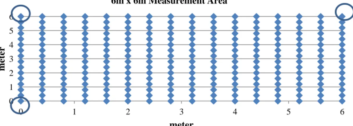
For testing performance of proposed systems, 256 data (features) are created within an interval of 0.4 meter in area of 6 square meters ( ) Figure 3.1. Each feature has vector.
Figure 3.1 6mx6m Measurement Area
3.2.2 12mx12m Measurement Area
For testing performance of proposed systems, 625 data (features) are created within an interval of 0.5 meter in area of 12 square meters ( (Figure 3.2)
0 1 2 3 4 5 6 0 1 2 3 4 5 6 m ete r meter 6m x 6m Measurement Area
20
Figure 3.2 12mx12m Measurement Area
3.2.3 24mx24m Measurement Area
For testing performance of proposed systems, 2397 data (features) are created within an interval of 0.5 meter in area of 24 square meters ( (Figure 3.3)
Figure 3.3 24mx24m Measurement Area 0 2 4 6 8 10 12 0 2 4 6 8 10 12 m ete r meter 12mx12m Measurement Area Distribution of 625 nodes -1 4 9 14 19 24 -1 4 9 14 19 24 m ete r meter) 24mx24m Measurement Area Distribution of 2397 nodes
21 3.3 Real Data Measurement
In order to compare algorithms with each other, real RSSI data were used. Kadir Has University’s canteen was chosen as a measurement area. Indoor environment are effected with person movement thus we choose holiday in order to avoid students’ effect on our environment. 6 square meter and 12 square meter areas were created. In 6 square meter area, 255 features and for 12 square meter are 444 features were used. Cell phone gathered RSSI values from each features inside of measurement area. During experiment, another cell phone (agent) is placed at the middle of measurement area and measured RSSI values from same node. In 6 square meter area agent coordinate is (3, 3) and for 12 square meter area agent coordinate is (6, 6). Agent provides to find “A” value from 4 different access points. Path Loss exponent are calculation with Brute Force technique for each RSSI values that measured. Brute Force algorithm is used to find optimum N values. Basically algorithm finds path loss exponent value for each access point. Algorithm find exponent until estimated distance and real distance is equal to each other for each RSSI values. Let assume there are measurement point. Path Loss exponent for access point is;
(3.1)
In 6mx6m environment, values respectively; -50.41, -49.09, -46.03, -47.65. Path Loss exponent is 2.97 for each access points.
In 12mx2m environment, values respectively; -42.28, -35.45, -32.72, -35.89. Path Loss exponent values respectively 2.97, 3.63, 3.40, 4.52
22
CHAPTER 4
Triangulation
Basic principle is using geometric properties of triangles to complete object location. There are two types of triangulation method; lateration and angulations. Lateration is using distance measurement, angulations is using primarily angle or bearing
measurements. [21]
4.1 Lateration
Lateration or Trilateraion is most well known estimation location in indoor positioning. Lateration is required three known positioned APs. We are collecting RSSI values from receivers. Measured RSSI values are converting into distance measurement by using path loss model. The path loss model shows the expected path loss in signal strength at a given distance (At one meter, dBm). Then known three distances from known APs are using Euclidean distance in order to estimate unknown object location Figure 4.1 [15].
23
The distance is estimated from RSSI values are used to compute centered in the three reverences anchor nodes. Ideally, the target should be intersection of the circles like in Figure 4.1.
From General Euclidean distance, radius can be find as
(4.1) After we re-arrange basic equation, we have matrix form;
= = * (4.2) Target location can be estimated after matrix equation is solved in (4.2)
= *
(4.3) 4.2 Angulations
Angulations are similar to Lateration, except instead of distance this method is using angle to determine position of object. This method is using AOA measurement so; it is required extra device to measure angles. Basically, the angle measurements at two APs and known AP locations are required. Then simple trigonometry can be applied to estimate distance. [15]
24 4.3 Test Bed
Triangulation algorithm requires 3 access points; and . In equation [4.1]; are representing ’s distance from measurement point. In order to find distance from measurement point, we are going to use Log-distance path loss model that we mentioned in chapter 2. Estimated distances in each feature were measured using equation (3.1).
4.4 Experimental Result
In chapter 3, synthetic data is created as triangulation method input. 6mx6m, 12mx12m and 24mx24m measurement areas are used. Coordinate of access points respectively: (0, 0), (6, 0), (6, 6).
For each experiment, equation (2.2), (3.1) and (4.3) are applied.
4.4.1 6m x 6m Measurement Area
Circle figures represent access point placement. There are 256 test nodes, however we ignore nodes where it is access point coordinates. 253 data features were used within an interval of 0.4 meter in an area of 6 square meters ( ).
Figure 4.3 6mx6m Measurement Area – Access Point Placement 0 1 2 3 4 5 6 0 1 2 3 4 5 6 m et er meter 6m x 6m Measurement Area
25 4.4.1.1 6mx6m Area (LOS Environment)
There are not any obstacles between transmitter and receiver in LOS environment. This model is representing when there is any signal loss in measurement area. Features’ real location is blue figure; estimated location’s are red figures.
Average is 0.0 meter, minimum error is -0.01 meter, maximum error is 0.01 meter and standard deviation is 0.00 meter. (Figure 4.4)
N value Average Error Minimum Error Maximum Error Standard Deviation
2.18 0.00 0.00 0.01 0.00
Figure 4.4 Experiment on LOS Environment (6mx6m)
4.4.1.2 6mx6m Area (0.5 dBm Noise)
This model is representing when there is 0.5 dBm signal loss in measurement area. Features’ real location is blue figure; estimated location’s are red figures.
Average is 0.42 meter, minimum error is 0.02 meter, maximum error is 1.82 meter, and standard deviation is 0.33 meter. (Figure 4.5)
0 1 2 3 4 5 6 7 0 1 2 3 4 5 6 7 m ete r meter
26
N Value Average Error Minimum Error Maximum Error Standard Deviation
2.18 0.42 0.02 1.82 0.33
Figure 4.5 Experiment on 0.5 Noise Environment (6mx6m) 4.4.1.3 6mx6m Area (1 dBm Noise)
This model is representing when there is 1 dBm signal loss in measurement area. Features’ real location is blue figure; estimated location’s are red figures.
Average is 0.86 meter, minimum error is 0.03 meter, maximum error is 4.01 meter, and standard deviation is 0.61 meter. (Figure 4.6)
N
value Average Error Minimum Error Maximum Error Standard Deviation
2.18 0.86 0.03 4.01 0.61
Figure 4.6 Experiment on 1 Noise Environment (6mx6m) -2 -1 0 1 2 3 4 5 6 7 -2 -1 0 1 2 3 4 5 6 7 8 m et er meter
0.5 dBm Noise Measurement Area
-4 -2 0 2 4 6 8 10 -4 -2 0 2 4 6 8 meter meter
27 4.4.1.4 6mx6m Area (1.5 dBm Noise)
This model is representing when there is 1.5 dBm signal loss in measurement area. Features’ real location is blue figure; estimated location’s are red figures.
Average is 1.35 meter, minimum error is 0.03 meter, maximum error is 7.01 meter, and standard deviation is 1.1 meter. (Figure 4.7)
N
value Average Error Minimum Error Maximum Error Standard Deviation
2.18 1.35 0.03 7.14 1.1
Figure 4.7 Experiment on 1.5 Noise Environment (6mx6m)
4.4.1.5 6mx6m Area (2 dBm Noise)
This model is representing when there is 2 dBm signal loss in measurement area. Features’ real location is blue figure; estimated location’s are red figures.
Average is 1.93 meter, minimum error is 0.04 meter, maximum error is 10.66 meter, and standard deviation is 1.79 meter. (Figure 4.8)
-8 -6 -4 -2 0 2 4 6 8 10 12 -4 -2 0 2 4 6 8 10 12 meter meter
28 N
value Average Error Minimum Error Maximum Error Standard Deviation
2.18 1.93 0.04 10.66 1.79
Figure 4.8 Experiment on 2 Noise Environment (6mx6m) 4.4.1.6 6mx6m Area (2.5 dBm Noise)
This model is representing when there is 2.5 dBm signal loss in measurement area. Features’ real location is blue figure; estimated location’s are red figures.
Average is 2.31 meter, minimum error is 0.04 meter, maximum error is 9.36 meter, and standard deviation is 1.93 meter. (Figure 4.9)
N
value Average Error Minimum Error Maximum Error Standard Deviation
2.18 2.31 0.04 9.86 1.93
Figure 4.9 Experiment on 2.5 Noise Environment (6mx6m) -10 -5 0 5 10 15 -10 -5 0 5 10 15 meter meter
2 dBm Noise Measurement Area
-10 -5 0 5 10 15 -10 -5 0 5 10 15 20 meter meter
29 4.4.1.7 6mx6m Area (3 dBm Noise)
This model is representing when there is 3 dBm signal loss in measurement area. Features’ real location is blue figure; estimated location’s are red figures.
Average is 2.94 meter, minimum error is 0.02 meter, maximum error is 18.31meter, and standard deviation is 2.91 meter. (Figure 4.10)
N
value Average Error Minimum Error Maximum Error Standard Deviation
2.18 2.94 0.02 18.31 2.91
Figure 4.10 Experiment on 3 Noise Environment (6mx6m)
4.4.1.8 6mx6m Area (3.5 dBm Noise)
This model is representing when there is 3.5 dBm signal loss in measurement area. Features’ real location is blue figure; estimated location’s are red figures.
Average is 3.65 meter, minimum error is 0.04 meter, maximum error is 30.50 meter, and standard deviation is 4.19 meter. (Figure 4.11)
-15 -10 -5 0 5 10 15 20 -15 -10 -5 0 5 10 15 20 25 meter meter
30 N
value Average Error Minimum Error Maximum Error Standard Deviation
2.18 3.65 0.04 30.50 4.19
Figure 4.11 Experiment on 3.5 Noise Environment (6mx6m) 4.4.1.9 6mx6m Area (4 dBm Noise)
This model is representing when there is 4 dBm signal loss in measurement area. Features’ real location is blue figure; estimated location’s are red figures.
Average is 4.30 meter, minimum error is 0.04 meter, maximum error is 28.38 meter, and standard deviation is 4.56 meter. (Figure 4.12)
In Figure 4.13, we restricted estimated location with measurement area. 177 nodes were out of area. Average is 2.05 meter, minimum error is 0.06, maximum error is 6.72 meter and standard deviation is 1.24 meter.
N
value Average Error Minimum Error Maximum Error Standard Deviation
2.18 4.30 0.04 28.38 4.56
Figure 4.12 Experiment on 4 Noise Environment (6mx6m) -30 -20 -10 0 10 20 30 -30 -20 -10 0 10 20 30 meter meter
3.5 dBm Noise Measurement Area
-30 -20 -10 0 10 20 30 -30 -20 -10 0 10 20 30 meter meter
31 N
value Average Error Minimum Error Maximum Error Standard Deviation
2.18 2.05 0.00 6.72 1.24
Figure 4.13 Experiment on 4 Noise Environment (6mx6m) - Recuirement 4.4.1.10 6mx6m Area (4.5 dBm Noise)
This model is representing when there is 4.5 dBm signal loss in measurement area. Features’ real location is blue figure; estimated location’s are red figures.
Average is 5.54 meter, minimum error is 0.33 meter, maximum error is 42.07 meter, and standard deviation is 7.05 meter. (Figure 4.14)
N
value Average Error Minimum Error Maximum Error Standard Deviation
2.18 5.54 0.33 42.07 7.05
Figure 4.14 Experiment on 4.5 Noise Environment (6mx6m) 0 1 2 3 4 5 6 7 0 1 2 3 4 5 6 7 m et er meter
Measurement Area 4 dBm Noise
-40 -30 -20 -10 0 10 20 30 40 50 -40 -30 -20 -10 0 10 20 30 40 50 meter meter
32 4.4.1.11 6mx6m Area (5 dBm Noise)
This model is representing when there is 5 dBm signal loss in measurement area. Features’ real location is blue figure; estimated location’s are red figures.
Average is 6.32 meter, minimum error is 0.14 meter, maximum error is 62.40 meter, and standard deviation is 7.26 meter. (Figure 4.15)
N
value Average Error Minimum Error Maximum Error Standard Deviation
2.18 6.32 0.14 62.40 7.26
Figure 4.15 Experiment on 5 Noise Environment (6mx6m)
4.4.1.12 Experiment with Real Data
In chapter 3, environment with real data is described. is used during experiment. Average is 2.32 meter, minimum error is 0.2 meter, maximum error is 10.13 meter, and standard deviation is 1.35 meter. (Figure 4.16)
-40 -30 -20 -10 0 10 20 30 40 50 -40 -30 -20 -10 0 10 20 30 40 50 meter meter
33
Average Error Minimum Error Maximum Error Standard Deviation
2.32 0.2 10.13 1.35
Figure 4.16 Experiment with Real Data (6mx6m)
4.4.2 12mx 12m Measurement Area
Circle figures represent access point placement. There are 625 test nodes, however we ignore nodes where it is access point coordinates. 623 data features were used within an interval of 0.5 meter in an area of 12 square meters ( ) Figure 4.17.
Figure 4.17 12mx12m Measurement Area-Access Point Placement -4 -2 0 2 4 6 8 10 12 0 2 4 6 8 10 12 14 meter meter
Measurement Area Algorithm Result
0 2 4 6 8 10 12 0 2 4 6 8 10 12 m et er meter 12mx12m Measurement Area Distribution of 625 nodes
34 4.4.2.1 12mx12m Area (LOS)
There are not any obstacles between transmitter and receiver in LOS environment. This model is representing when there is any signal loss in measurement area. Features’ real location is blue figure; estimated location’s are red figures.
Average is 0.0 meter, minimum error is 0.00 meter, maximum error is 0.02 meter and standard deviation is 0.00 meter. (Figure 4.18)
N
value Average Error Minimum Error Maximum Error Standard Deviation
2.18 0,00 0.00 0,02 0,00
Figure 4.18 Experiment on LOS Environment (12mx12m) 4.4.2.2 12mx12m Area (0.5 dBm Noise)
This model is representing when there is 0.5 dBm signal loss in measurement area. Features’ real location is blue figure; estimated location’s are red figures.
Average is 0.83 meter, minimum error is 0.03 meter, maximum error is 4.54 meter and standard deviation is 0.63 meter. (Figure 4.19)
-2 0 2 4 6 8 10 12 14 -2 0 2 4 6 8 10 12 14 meter meter
35 N
value Average Error Minimum Error Maximum Error Standard Deviation
2.18 0.83 0.03 4.54 0.63
Figure 4.19 Experiment on 0.5 dBm Noise Environment (12mx12m) 4.4.2.3 12mx12m Area (1 dBm Noise)
This model is representing when there is 1 dBm signal loss in measurement area. Features’ real location is blue figure; estimated location’s are red figures.
Average is 1.72 meter, minimum error is 0.05 meter, maximum error is 8.08 meter and standard deviation is 1.23 meter. (Figure 4.20)
N
value Average Error Minimum Error Maximum Error Standard Deviation
2.18 1.72 0.05 8.08 1.23
Figure 4.20 Experiment on 1 dBm Noise Environment (12mx12m) -5 0 5 10 15 20 -5 0 5 10 15 20 meter meter
0.5 dBm Noise Measurement Area
-10 -5 0 5 10 15 20 -5 0 5 10 15 20 meter meter
36 4.4.2.4 12mx12m Area 1.5 dBm
This model is representing when there is 1.5 dBm signal loss in measurement area. Features’ real location is blue figure; estimated location’s are red figures.
Average is 2.59 meter, minimum error is 0.02 meter, maximum error is 24.46 meter and standard deviation is 2.26 meter. (Figure 4.21)
N
value Average Error Minimum Error Maximum Error Standard Deviation
2.18 2.59 0.02 24.46 2.26
Figure 4.21 Experiment on 1.5 dBm Noise Environment (12mx12m) 4.4.2.5 12mx12m Area 2dBm
This model is representing when there is 2 dBm signal loss in measurement area. Features’ real location is blue figure; estimated location’s are red figures.
Average is 3.60 meter, minimum error is 0.08 meter, maximum error is 27.14 meter and standard deviation is 2.94 meter. (Figure 4.22)
-15 -10 -5 0 5 10 15 20 25 30 -20 -10 0 10 20 30 meter meter
37 N
value Average Error Minimum Error Maximum Error Standard Deviation
2.18 3.60 0.08 27.14 2.94
Figure 4.22 Experiment on 2 dBm Noise Environment (12mx12m)
4.4.2.6 12mx12m Area 2.5 dBm
This model is representing when there is 2.5 dBm signal loss in measurement area. Features’ real location is blue figure; estimated location’s are red figures.
Average is 4.64 meter, minimum error is 0.04 meter, maximum error is 36.81 meter and standard deviation is 4.34 meter. (Figure 4.23)
N
value Average Error Minimum Error Maximum Error Standard Deviation
2.18 4.64 0.04 36.81 4.34
Figure 4.23 Experiment on 2.5 dBm Noise Environment (12mx12m) -20 -10 0 10 20 30 40 -20 -10 0 10 20 30 m et er meter
2 dBm Noise Measurement Area
-40 -30 -20 -10 0 10 20 30 40 -30 m -20 -10 0 10 20 30 40 50 e te r meter
38 4.4.2.7 12mx12m Area 3 dBm
This model is representing when there is 3 dBm signal loss in measurement area. Features’ real location is blue figure; estimated location’s are red figures.
Average is 5.99 meter, minimum error is 0.05 meter, maximum error is 95.27 meter and standard deviation is 7.55 meter. (Figure 4.24)
In Figure 4.25, we restricted estimated location with measurement area. 344 nodes were out of area. Average is 3.55 meter, minimum error is 0.00, maximum error is 11.88 meter and standard deviation is 2.45 meter.
N
value Average Error Minimum Error Maximum Error Standard Deviation
2.18 5.99 0.05 95.27 7.55
Figure 4.24 Experiment on 3 dBm Noise Environment (12mx12m) -120 -100 -80 -60 -40 -20 0 20 40 60 80 -80 -60 -40 -20 0 20 40 60 m et er meter
39 N
value Average Error Minimum Error Maximum Error Standard Deviation
2.18 3.55 0.00 11.88 2.45
Figure 4.25 Experiment on 3 dBm Noise Environment (12mx12m) 4.4.2.8 12mx12m Area 3.5 dBm
This model is representing when there is 3.5 dBm signal loss in measurement area. Features’ real location is blue figure; estimated location’s are red figures.
Average is 6.87 meter, minimum error is 0.10 meter, maximum error is 74.84 meter and standard deviation is 7.60 meter. (Figure 4.26)
N
value Average Error Minimum Error Maximum Error Standard Deviation
2.18 6.87 0.10 74.84 7.60
Figure 4.26 Experiment on 3.5 dBm Noise Environment (12mx12m) 0 2 4 6 8 10 12 14 0 2 4 6 8 10 12 14 m ete r meter
Measurement Area Triangulation-Recurement
-40 -20 0 20 40 60 80 -60 -40 -20 0 20 40 60
40 4.4.2.9 12mx12m Area 4 dBm
This model is representing when there is 4 dBm signal loss in measurement area. Features’ real location is blue figure; estimated location’s are red figures.
Average is 8.98 meter, minimum error is 0.07 meter, maximum error is 218.34 meter and standard deviation is 12.49 meter. (Figure 4.27)
N
value Average Error Minimum Error Maximum Error Standard Deviation
2.18 8.98 0.07 218.34 12.49
Figure 4.27 Experiment on 4 dBm Noise Environment (12mx12m) 4.4.2.10 12mx12m Area 4.5 dBm
This model is representing when there is 4.5 dBm signal loss in measurement area. Features’ real location is blue figure; estimated location’s are red figures.
Average is 10.71 meter, minimum error is 0.07 meter, maximum error is 123.22 meter and standard deviation is 13.94 meter. (Figure 4.28)
-100 -50 0 50 100 150 200 -200 -150 -100 -50 0 50 100 150 meter meter
![Figure 1.1 Forecast of global RLTS market by value $US millions [3] Also IDTechEx claims that $10 billion addressable market waits for RLTS](https://thumb-eu.123doks.com/thumbv2/9libnet/4319282.70676/22.892.271.729.768.1070/figure-forecast-global-market-millions-idtechex-billion-addressable.webp)