Applications of machine learning in classification of biological data

(1)

KADİR HAS UNIVERSITY

GRADUATE SCHOOL OF SCIENCE AND ENGINEERING

PROGRAM OF COMPUTATIONAL BIOLOGY AND BIOINFORMATICS

APPLICATIONS OF MACHINE LEARNING IN

CLASSIFICATION OF BIOLOGICAL DATA

AYLİN BİRCAN

MASTER’S THESIS

(2)

Ay lin Bi rcan M. Sc . Th es is 20 18

(3)

APPLICATONS OF MACHINE LEARNING IN

CLASSIFICATION OF BIOLOGICAL DATA

AYLİN BİRCAN

MASTER’S THESIS

Submitted to the Graduate School of Science and Engineering of Kadir Has University in partial fulfillment of the requirements for the degree of Master’s in the Program of

Computational Biology and Bioinformatics

(4)

(5)

(6)

ABSTRACT

Machine learning enables computers learn from the data. It has a wide range of application areas. Computational biology and bioinformatics are some areas in which machine learning applications provide accurate solutions to problems. Different types of machine learning tasks are summarized as supervised, semi-supervised, unsupervised and reinforcement learning. In this thesis, we focus on supervised machine learning tasks on biological datasets. We applied multiple machine learning approaches to different datasets. K-nearest neighbor, softmax classification, neural networks approaches are considered. Moreover, we discussed suitable algorithms and acceptable machine learning models to classify a biological data.

(9)

BİYOLOJİK VERİLERİN SINIFLANDIRILMASINDA MAKİNE ÖĞRENİMİNİN KULLANIMI

ÖZET

Makine öğrenimi, bilgisayarların veriden öğrenmesini sağlar. Çok çeşitli uygulama alanlarına sahiptir. Hesaplamalı biyoloji ve biyoinformatik, makine öğrenimi uygulamalarının problemlere doğru çözümler sağladığını gösteren bazı alanlardır. Farklı makine öğrenimi algoritmaları, denetimli, yarı denetimli, denetimsiz ve takviye öğrenme olarak özetlenmiştir. Bu tezde, biyolojik veri kümeleri üzerinde denetlenen makine öğrenimi algoritmalarına odaklanıldı. Farklı veri kümelerine çoklu makine öğrenme yaklaşımları uygulanıldı. K-en yakın komşu, softmax sınıflandırması, sinir ağları yaklaşımları kullanıldı. Ayrıca, bir biyolojik veriyi sınıflandırmak için uygun algoritmalar ve kabul edilebilir makine öğrenme modelleri tartışıldı.

(10)

ACKNOWLEDGEMENTS

I would like to thank to my adviser (Assoc. Dr. Cem Özen) for his guidance, support and patience. I would also like to thank to all faculty members of Computational Biology and Bioinformatics Department. Last, but not least, I would like to thank to my dearest husband, my family and friends for their support and love. Thank you... Very much indeed.

(11)

LIST OF TABLES

Table 3.1: The training and the testing accuracies of datasets with the softmax

classification algorithm………....34 Table 3.2: Architecture of neural network models………...…...38 Table 3.3: Accuracy results by using cross-validation method and 10th_method

parameters...46 Table 3.4: Architecture of neural network models………...48

(12)

LIST OF FIGURES

Figure 1.1: Schematic representation of linear regression model...7

Figure 1.2: Linear regression problem example...9

Figure 1.3: Gradient descent...10

Figure 1.4: Schematic representation of linear regression model...11

Figure 1.5: Sigmoid function...11

Figure 1.6.A&B&C: Softmax examples with different classes...12-13 Figure 1.7: Schematic of artificial neural network with one hidden layer and three units...14

Figure 1.8: Schematic of one unit operations...15

Figure 1.9: A convolutional matrix………...18-19 Figure 1.10: Elliptical contours after the projection mapping of the cost function...20

Figure 1.11: Data are artificially made by using Sklearn make_blobs dataset...22

Figure 1.12 A&B&C: Model without L2 regularization...22

Figure 1.13 A&B&C: Model with L2 regularization λ=0.01...23

Figure 1.14 A&B&C: Model with L2 regularization λ=0.1...24

Figure 1.15: Neural network with two hidden layers...25

Figure 1.16: Computation graph example...28

Figure 3.1.A&B: The softmax classification approach on the yeast dataset...35

Figure 3.2.A&B: Softmax Classification approach on breast cancer dataset...35

Figure 3.3.A&B: The softmax classification approach on the determination of cancer type based on the gene expression dataset...36

Figure 3.4.A&B: The softmax classification approach on the epileptic seizure recognition dataset………....………...36

Figure 3.5: Misclassification error vs. number of neighbors...37

Figure 3.6.A&B: Model 1...39

(13)

Figure 3.14.A&B: Model 9...43-44 Figure 3.15.A&B: Model 10...44

Figure 3.16: Confusion matrix for themodel 10 on the yeast dataset...45

(14)

1. INTRODUCTION

1.1 What Is Machine Learning

Machine learning is a branch of computer science that enables computers to learn from the data. By learning from the data, we mean that the computers improve their ability to solve certain problems using the data and they learn from it via programming using specific algorithms and frameworks. In order to achieve successful learning, statistical methods are heavily used in these algorithms (Géron, 2017).

Arthur Samuel coined the term "machine learning" in 1950s (Samuel, 1988). Machine learning has been emerged from the early scientific research of computational learning, in particular, pattern recognition. Pattern recognition is the study of patterns of the data, i.e., regular and irregular values. Note that the terms machine learning and pattern recognition can be used interchangeably because they "can be viewed as two facets of the same field" since machine learning is originated from computer science and pattern recognition is originated from engineering (Bishop, 2006). Note also that the aim of machine learning is to devise algorithms that can make accurate predictions based on the given data where building explicit computer programs is impracticable (Kohavi and Provost, 1998). Therefore, one can say that machine learning is different from traditional software programming because in this case computers are not explicitly programmed. In traditional software programming, input and output types are pre-determined. Every condition (such as if/else statements, switch statements etc.) based on the input is checked explicitly in the computer code. This is how the evaluation is done and the output is computed. It does not learn from the input and it gives the same output every time same input is given. However, in machine learning, algorithms learn from data without being explicitly programmed. For instance, creating a spam filter is a good example that

(15)

illustrates the difference. The spam filter learns from previous e-mail messages in the inbox that are marked as spam by its user. As e-mails which have different content marked as spam, the algorithm learns from these marked e-mails and start to mark new e-mails with the same content as spam without being updated (Géron, 2017). The spam filter example is also important for illustrating the use of pattern recognition in machine learning algorithms. It determines the spam messages according to the patterns emerged in previous spam messages.

One of the reasons behind the advancement of machine learning in the last decade is due to the improvement of data and its related technologies. In today's world, a huge amount of data is produced every day and by the increased capacity of computers, data can be stored. Furthermore, many datasets are publicly available in internet databases. Thus, we need not only accurate but also fast and efficient algorithms to interpret this data. Machine learning algorithms provide efficient solutions to these complex problems. They have a wide range of application areas. For instance, search engines, financial applications, medical diagnoses; biological problems are some examples of areas where machine learning applications are used.

In particular, there are a lot of biological databases available on the internet. These databases provide protein sequences, nucleotide sequences, gene expression data etc. For example, National Center for Biotechnology Information Center provides a lot of resources such as Genes and Expression, proteins. Accessing and producing new data is easier than ever. The main question is how the data is used to obtain biologically meaningful results within a reasonable time period with low computational cost. For instance, the amino acid sequence of a protein provides important information about the function of the protein. Proteins are transferred into different organelles in the cell. The amino acid sequence of a protein determines where the protein will function in the cell. Determination of a protein location in the cell can be solved by using machine learning algorithms (Horton and Nakai, 1996).

Machine learning is also used to diagnose diseases. Cancer types, diabetic retinopathy are some diseases that are studied by using machine learning algorithms. Retina images are

(16)

used to diagnose the level of the diabetic retinopathy by using deep learning approach. Convolutional neural networks perform with high accuracy on image datasets (Ching et al., 2018). Different cancer types can be determined by using gene expression levels (Weinstein et al., 2013).

Machine learning differentiates based on the tasks. There are four different classes of machine learning tasks. In this thesis, we focus on supervised machine learning classification on different biological datasets. Each dataset requires a different classification algorithm to achieve the desired result.

1.2 Types of Machine Learning Tasks

Machine learning can be categorized based on tasks as (Géron, 2017): -Supervised machine learning

-Unsupervised machine learning -Semi-supervised machine learning -Reinforcement machine learning

Machine learning algorithm learns from the data that is called the training set. The training set is used to train the algorithm which means the algorithm learns how to map inputs to outputs. Each element in the training set is called the training sample or the training instance. In a dataset, all samples have the same features. For example, classification of objects from images can be a machine learning problem. For this specific problem, pixel intensities of the images will be the features and each image will be the sample. In the training process, the algorithm learns to map these pixel intensities to the objects in the image. After the algorithm is trained with the training set, it is tested on a different dataset which is not used to train the model. This dataset is called the testing set. The model is tested on the testing set to measure the performance of the model.

In supervised machine learning, correct outputs (labels) of the input samples are given and the algorithm learns the relationship between inputs and outputs. It is like learning

(17)

the questions while having the correct answers. Supervised machine learning tasks are divided into two categories based on the output type of the given dataset. Classification and regression are two supervised machine learning tasks.

In the classification task, machine learning algorithm is trained with a dataset which has discrete categories as labels. Then the algorithm is expected to predict to which category a new data belongs. If the given data has two categories to classify the samples, it is called binary classification. More than two categories to classify the samples are called multi-class multi-classification. Determination of a person has diabetes or not is a binary multi-classification example. If the problem is the determination of a person has diabetes, cancer or a heart disease, then the problem is multi-class classification. Each disease represents a category. Regression is another task in supervised machine learning. Unlike classification tasks where the outputs are discrete categories, the output of regression tasks is a real number that means that the algorithm maps the given input to a real-valued output. Predicting house prices on the basis of the given features is a common regression problem example. Price of a house is not a category, but it has a real value.

Unlike supervised machine learning, in unsupervised learning, right labels of the input data are not given. The algorithm finds the correct structure in the data without training with labels. Like supervised machine learning classification and regression tasks, unsupervised machine learning has different tasks.

Clustering is one example of unsupervised machine learning tasks. In clustering, machine learning algorithm finds out how the given dataset can be divided into sub-classes which are called clusters. Specific features that are common in the clusters are not given initially, the algorithm finds out these common features (Dasgupta and Nath, 2016). Determining user groups who visit a website based on common features they share is a clustering example (Géron, 2017).

Dimensionality reduction is another task of unsupervised machine learning. In this case, some features are reduced by avoiding loss of information. If there are features which are

(18)

correlated with each other, they can be collected as one feature, so the dataset will be minimized. For example, age and mileage of a car are two features which are correlated with each other, so they can be collected together as one feature (Géron, 2017).

Semi-supervised learning includes both labeled data and unlabeled data. Supervised and unsupervised learning are the two parts of semi-supervised learning. (Dasgupta and Nath, 2016).

Reinforcement machine learning is quite different from other machine learning tasks. The learning system is called agent and the learned strategy is called policy. Based on the decisions that the system made, it obtains reward and punishment. Reinforcement machine learning is used in walking robots (Géron, 2017).

1.3 Exploring and Processing Data

In any type of machine learning algorithm organizing given data is very important. In the training dataset, all instances must have every feature. In some datasets, there could be missing features for some instances. Before applying any algorithm to this dataset, missing features have to be considered. If the missing feature is not a very important feature and it is not available for most of the samples, then this feature can be excluded. However, if the missing feature is an important feature, then it can be filled with the most frequent value among other instances. In addition, there are more complex methods available that fill the missing features in the dataset (Mitchel, 1997). Having a dataset that has no missing attributes among samples is not enough to start training a model.

In order to make training set optimal, feature scaling is needed because usually, machine learning algorithms do not work correctly without scaled features. Optimization algorithms, such as the gradient descent, may be run with suboptimal efficiency. Min-max scaling, where all features scale to the range of 0 and 1, and standardization, where we subtract the mean from features and divide them by the standard deviation, are two popular feature scaling methods. Moreover, after the feature scaling gradient descent algorithm converges to the global minimum faster.

(19)

Datasets are available in different repositories such as Kaggle and University of California Irvine machine learning repository. In this thesis, used datasets from California Irvine machine learning repository. The datasets which we used do not contain missing attributes and we did not extract any sample or any feature. We focused on data belonging to several different problems. One of them is the determination of cancer types based on gene expression levels. The Cancer Genome Atlas (TCGA) Research Network has studied different tumor types (Weinstein et al., 2013). These studies provide a dataset of gene expression levels of tumor types. We used this dataset to classify the tumor type based on the gene expression levels by using the softmax classification algorithm. Another problem we have chosen is the determination of protein locations in yeast. Proteins are transferred into different organelles in the cell. The amino acid sequence of a protein determines where the protein will function in the cell (Horton and Nakai, 1996). We used different machine learning approaches in this dataset.

Breast cancer Wisconsin (diagnostic) dataset which includes features extracted from the image of breast mass (Street et. al., 2009) is used as the third problem. The problem constitutes the classification of two different breast tumors.

Lastly, we have considered a dataset on epileptic seizure recognition. This dataset includes the brain activity of patients, that are recorded with EEG (Andrzejak et. al., 2001). We aimed to determine if the patients have an epileptic seizure or they are healthy individuals.

1.4 Supervised Machine Learning Models

There are different supervised machine learning models. Linear regression, logistic regression, k-nearest neighbors, decision trees and random forests, support vector machines, and artificial neural networks are some of the most well-known supervised machine learning algorithms. Each supervised machine learning model can be effective for the different type of problems. Logistic regression and linear regression supervised

(20)

machine learning models are efficient for linearly separable datasets. As samples are clustered, the problem is not linearly separable. It makes logistic regression and linear regression models inefficient. For big and linearly inseparable data, much more advanced models like artificial neural networks are needed. All supervised machine learning models are trained with data which labels are already known.

1.4.1 Linear Regression

Linear regression is a linear function which takes input features and produces output values. Linear regression gives a real number as an output; however, this model can be used for classification tasks as well. To use linear regression model for classification problems, we can determine a threshold. For example, we can say that one sample belongs to class A if the output value is above the threshold. If the output value is below the threshold then the sample is not in class A.

Figure 1.1: Schematic representation of linear regression model

𝑥: input values 𝑦̂: prediction value 𝑦: ground truth value ℎ: hypothesis function 𝑤: weight

(21)

ℎ = 𝑦̂ = 𝑤)_{𝑥 + 𝑏 (1.1)} Let us say we have data with m training examples with n features such that:

𝑚: number of training examples 𝑛: number of features

𝑋 ∈ ℝ0×2, _{𝑌 ∈ ℝ}4×2

Training set: {(𝑥₄(4), 𝑦₄(4)), (𝑥₉(9), 𝑦₉(9)), … , (𝑥₀(2), 𝑦₀(2))} X and Y will be presented as:

𝑋 = < | | | 𝑥(4) _𝑥(9) _{… 𝑥}(2) | | | > 𝑌̂ = [𝑦(4)̂ _{, 𝑦}(9)̂ _{, … , 𝑦}(2)̂ _]

As a supervised machine learning algorithm, the purpose is to train the model with the training examples and find 𝑤 and 𝑏 values, so that predicted values 𝑦̂_{are close to the} labels 𝑦.

After the algorithm is trained with examples, the difference between predicted values and labels must be found. The loss function is the difference between the predicted and the actual value for one sample. The cost function is the general form of the loss function which captures all samples in the dataset. The squared error function is commonly used cost function for linear regression problems. The loss function and the cost function for linear regression are defined as below:

𝐿(𝑦, 𝑦̂) = (𝑦(B)_{− 𝑦}(B)̂ ₎9 _(1.2) _{𝐽 =} 4

2_BF4∑ 2

𝐿(𝑦(B)_{, 𝑦}̂ (B)₎ _(1.3)

(22)

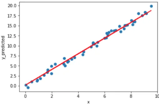
Figure 1.2: Linear regression problem example with one feature 𝑥 and 50 number of examples. Dataset is created by using numpy random number generator. Model is built by using Tensorflow (Abadi et al., 2015). Red line shows the decision boundary of the

algorithm.

After the model is trained on the training dataset, the cost function has to be minimized. Starting with some random 𝑤, 𝑏 values, an optimization algorithm iteratively changes the 𝑤, 𝑏 values to reduce 𝐽(𝑤, 𝑏) until it will end up at a minimum. Learning rate (𝛼) determines each step taken while reducing the cost function. Value of the learning rate will determine how long will it take to reach a minimum value even it can even reach the minimum value.

The optimization algorithm will update 𝑤 and 𝑏 values by taking partial derivative with respect to 𝑤 and 𝑏. 𝑤₄: = 𝑤₄− 𝛼_IKIJ L 𝑏4: = 𝑏4− 𝛼 IJ IML 𝑤₀: = 𝑤₀− 𝛼_IKIJ N 𝑏0: = 𝑏0 − 𝛼 IJ IMN

In order for the search algorithms to work efficiently and guarantee to reach the global maximum, the cost function needs to be a convex function of 𝑤 and 𝑏 values. A convex

(23)

function will then converge to the global minimum by a proper choice of the learning rate.

Figure 1.3: Gradient descent (Géron, 2017).

1.4.2 Binary Classification: Logistic Regression

Logistic regression algorithm is a binary classification algorithm. For binary classification task on a dataset, linear regression algorithm would not produce an efficient decision boundary. For binary classification, the output value is expected between 0 and 1. The value will be 1 for the correct label and 0 for the other label. However, linear regression model will produce values below 0 and above 1, so it is not an effective model for binary classification problems. An outlier in the dataset will shift the decision boundary of the linear regression dramatically when it is used for classification tasks by applying a threshold. In general, for binary classification problems the logistic regression is a more appropriate algorithm than the linear regression.

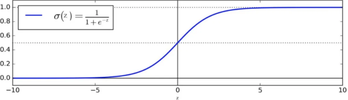
The logistic regression algorithm predicts the probability that 𝑦 = 1, conditional on given input 𝑥 and the model parameters 𝑤 and 𝑏 that is:

𝜎(𝑥) = 𝑝(𝑦 = 1|𝑥; 𝑤, 𝑏) 0 < 𝜎(𝑥) < 1 𝑦 = 0 or 𝑦 = 1

(24)

Figure 1.4: Schematic representation of linear regression model 𝑦̂ = 𝜎(𝑧) where 𝑧 = 𝑤)_{𝑥 + 𝑏}

Figure 1.5: Sigmoid function

To optimize the logistic regression algorithm, a cost function is needed. Squared error function used for linear regression model is not appropriate for logistic regression function, because it will produce lots of local minimum values when applied to logistic regression and gradient descent algorithm may not reach the global minimum. For this reason, another cost function is needed to guarantee that the gradient descent algorithm eventually reaches the global minimum. Such a cost function is given below:

𝐽(𝑤) =₂4 ∑ BF4

2

(25)

1.4.3 Multi-Class Classification: Softmax Function

The logistic regression algorithm is used for binary classification problems. If there are multiple labels (classes), then the logistic regression algorithm is not useful. Instead, the softmax classification function is used for multi-label classification problems. The function will give the probabilities belonging to each class. The softmax function is given by:

𝑔(𝑧) =_∑_Z[\_Z_]^

`aL for 𝑗 = 1,2, … … . , 𝐶 (1.5)

where 𝐶 is the output class index.

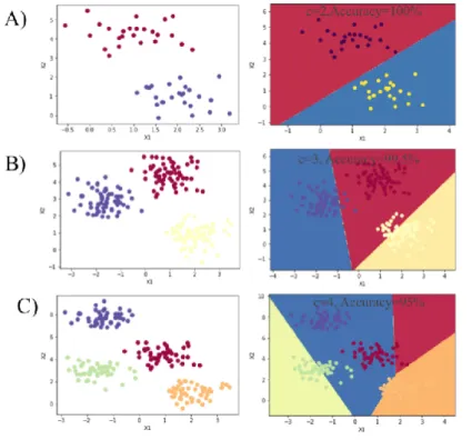
Figure 1.6.A&B&C: Softmax Examples with different classes. Graphs on the left shows data before any algorithm is applied. Linear decision boundaries between any

two classes. Data are artificially made by using Sklearn make_blobs dataset (Pedregosa et al., 2011).

(26)

Figure 1.6.A Softmax activation function example with two classes and accuracy is 100%.

Figure 1.6.B Softmax activation function example with three classes and accuracy is 99.5%

Figure 1.6.C Softmax activation function example with three classes and accuracy is 95.0%

By using Sklearn make_blobs dataset property (Pedregosa et al., 2011), different datasets with the different number of classes are prepared to visualize how softmax activation function is working. As it is shown in Figure 1.6.A&B&C, softmax activation function separates linearly different output classes. There is a linear decision boundary between any two different classes. Dots show the data points and linear lines show the decision boundaries between different classes.

1.4.4 Nearest neighbor classification: K-nearest neighbors

K-nearest neighbor is one of the simplest machine learning algorithms. In classification problems, K is a user-defined parameter. In order to identify the label of a query instance, the distance between the query instance and training instances in which labels are known is calculated. The label of the query instance depends on the chosen K value. If K is taken as 1, then the label of the query instance will be same as the label of the closest training instance. If K is larger than 1, then the distances between the query instance and training instances with known labels are calculated. Then the query point will be classified as the most frequent label in the K number of training instances that are nearest to the query point. Note that the training instances are labeled vectors in multidimensional space. One of the most popular distance functions is the Euclidean distance (Mitchel, 1997). One problem with the K-nearest neighbor method is the overfitting problem.

(27)

1.5 Neural Networks

1.5.1 Feed-Forward Neural Networks

Neural networks algorithms are inspired by the neural network in human brain, in which a neuron takes inputs through the dendrites, sum them in the cell body and gives its output to other neurons through the axon. Similar to the neurons in the brain, an artificial neuron takes its input from a set of neurons, perform some operations and give its output (Budama and Locascio, 2017).

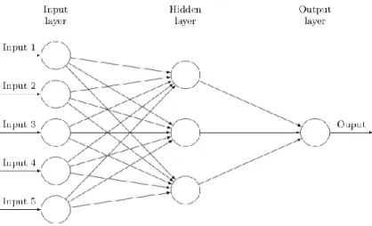
General visualization of neural networks is shown below:

Figure 1.7: Schematic of artificial neural network with one hidden layer and three units Every unit of every layer performs a linear mapping, then sends this result into a nonlinear function. The output of the unit is the output of the nonlinear function. This

(28)

Figure 1.8: Schematic of one unit operations

Let’s say we have a single training example with three features as 𝑥 and a neural network with 2 hidden layers with three units in each and an input layer and an output layer. 𝑥 = [𝑥₄, 𝑥₉, 𝑥_f] = 𝐴[h] _{is the input layer}

𝑤 = [𝑤4, 𝑤9, 𝑤f] is the weight matrix

As we define 𝑤_B(i) is the unit i in layer j, then we can define 𝑧 and activation function 𝑎 for the units of the first layers as follows:

First unit of the first layer 𝑧 and 𝑎 will be: z1(1) =w11(1)x1+w12(1)x2+w13(1)x3+b1(1)

a1(1) =g(z1(1))

Second unit of the first layer 𝑧 and 𝑎 will be: z2(1) =w21(1)x1+w22(1)x2+w23(1)x3+b2(1)

a2(1) =g(z2(1))

Third unit of the first layer z and a will be: z3(1) =w31(1)x1+w32(1)x2+w33(1)x3+b3(1)

a3(1) =g(z3(1))

Then we can generalize as follows;

𝑍[4] _{= 𝑊}[4]_𝐴[h]_{+ 𝑏}[4]_and 𝐴[4] _{= 𝑔(𝑍}[4]_{) is the output of the first layer} 𝑍[9] _{= 𝑊}[9]_𝐴[4]_{+ 𝑏}[9]_and 𝐴[9] _{= 𝑔(𝑍}[9]_{) is the output of the second layer} 𝑍[f] _{= 𝑊}[f]_𝐴[9]_{+ 𝑏}[f]_and 𝐴[f] _{= 𝑔(𝑍}[f]_{) is the output of the third layer}

In this example, the third layer is the output layer. In the output layer activation function will be different than the activation functions in the hidden layers.

(29)

There are several different activation functions. One of them is the restricted linear unit (ReLU), 𝑔(𝑧) = 𝑚𝑎𝑥(0, 𝑧). The ReLU has zero value for negative 𝑧 values and it takes values of 𝑧 as 𝑧 is greater than zero. Another activation function is the tanh function, 𝑔(𝑧) = 𝑡𝑎𝑛ℎ(𝑧). This function takes values between -1 and 1. It is centered at zero. Although, one usually has a freedom in the choice of the activation functions to be used in the hidden units, the type of the activation function in the output layer is determined by the problem; hence, for binary classification problems the sigmoid function, and for multiclass classification problems, the softmax function is used.

The input data is taken through the input layer and then propagates to the units in each hidden layer. The output of each hidden layer depends on the output of the previous hidden layer. Finally, the output is produced in the output layer. This process is called forward propagation.

Backward propagation is the process of computing the contribution of each unit of each hidden layer to the error. As in the other machine learning algorithms, a cost function minimizes the difference between predicted value and ground truth value. In order to minimize the error, an optimization algorithm is used to update 𝑤 and 𝑏 values. In neural networks the predicted value comes from computations in each unit of each layer. The algorithm uses the chain rule from calculus to compute the derivative. The chain rule is a tool used for computing the derivative of function compositions which basically states that the derivative of a function composition 𝑓 ∘ 𝑔 is the product of 𝑓p_{(𝑔) and 𝑔}p_. Therefore, we compute the derivatives of a layer using the derivatives of previous layers. The most important advantage of neural networks over simple sigmoid or softmax units is that, although the sigmoid and the softmax functions can separate data through linear decision boundaries only, a neural network can separate data by non-linear decision boundaries.

(30)

1.5.2 Convolutional Neural Networks

A robust human brain performs almost perfectly in visual detection tasks. People can

easily know what is seen in an image. This can be a cat, a face, a car or an object. Human brain easily identifies objects. This process is straightforward for humans. However, it is a complicated and hard task to perform for a computer. A computer identifies an image as a matrix. Every image has a width, height, and a color channel. Black and white images have height, width, and one-color channel. If the image is colorful, then it has the width, height and three-color channels. These color channels are red, green and blue. A computer identifies an image as a matrix that is composed of numbers. These numbers range between 0 and 255 and show the intensities of each pixel. When there is a high resolution, colorful image, then it is represented as a matrix with a dimension like 1000𝑥1000𝑥3. When feedforward neural networks algorithm is applied to such a matrix, there will be a huge number of features as an input vector. Adding hidden layers and units in the algorithm will produce huge number of weights. This process has high computational cost and it is not an effective process for image detection.

An effective method for image detection is inspired by the functioning of the brain. Some neurons in the brain detect the edges of an image (Hubel et. al., 1959). Edge detection is applied in machine learning by adding filters to the image. A filter is a matrix with weights. The user chooses the dimension of the matrix. Weights of the matrix can be learned with backward propagation. A filter matrix is set on an image matrix and convolutional operation is applied. Convolutional operation is element-wise multiplication and summation of the results of the multiplication. Filter matrix is set on the image matrix and convolutional operation is processed, then the filter matrix is slide through the right and down until it covers the whole image matrix. The filter can slide by one step through right and down, or it can slide by a certain distance. It is called stride, 𝑠 (Budama and Locascio, 2017). Stride is a hyperparameter of the model.

Padding is another hyperparameter of convolutional neural networks. When a filter matrix is set on an image matrix, numbers on the edges are taken once, however, numbers in the middle sides of the matrix are used multiple times. As a filter matrix is applied on an

(31)

image matrix, size of the output matrix is reduced. For example, when a filter with 3𝑥3 dimension is applied on a 6𝑥6 image matrix with stride 1, the output matrix will have a 4𝑥4 dimension. Reducing the dimension of the input matrix could cause loss of the feature information. To reduce information loss and protect the input dimension, one layer is added to the edges of the matrix. This process is called padding, 𝑝 (Budama and Locascio, 2017).

Figure 1.9 shows a 5𝑥5𝑥3 dimensional matrix. Padding, 𝑝 is one and stride 𝑠 is two in this example. In the figure, two different 3𝑥3𝑥3 dimensional filter matrices are shown. At the upper right, result of the first filter matrix applied to the first upper left of the image matrix is shown. At the bottom right, the result of the second filter matrix applied to first upper left of the image matrix is shown. Because there are two filter matrices are applied to the image matrix with 𝑝 is one and 𝑠 is two, the dimension of the output matrix will be 3𝑥3𝑥2.

(32)

Figure 1.9: A convolutional matrix with 5𝑥5𝑥3 dimension. Two different 3𝑥3𝑥3 filter matrices are applied with 𝑝 is 1 and 𝑠 is 2. Result of the first upper left of the convolutional matrix is shown on the upper right and result of the first upper left of the

convolutional matrix is shown on the bottom right (Budama and Locascio, 2017).

1.6 Training Neural Networks

1.6.1 Gradient descent

The gradient descent algorithm is an optimization algorithm which is used to minimize the cost function. As an illustration of gradient descent, we start with the most basic case where we have only two features. Therefore, we have two weights 𝑤₄ and 𝑤₉. Then the cost function is going to be a bowl shaped in three-dimensional space where 𝑥 axis and 𝑦 axis correspond to 𝑤₄ and 𝑤₉. Vertical 𝑧 axis corresponds to the cost function. The projection of this three-dimensional object to the 𝑧 axis will produce contours of elliptical shape. Moreover, since out three-dimensional object is bowl shaped with the minimum at its center, the minimum point is the center of elliptical contours in our projection (Buduma and Locascio, 2017).

(33)

Figure 1.10: Elliptical contours after the projection mapping of the cost function (Buduma and Locascio, 2017).

The Gradient descent algorithm will update weight parameters by taking partial derivatives of the cost function with respect to the weights after every iteration. If the gradient descent algorithm uses all samples in every iteration, it is called the batch gradient descent. It is effective to use all samples when the cost function is low dimensional. However, in high dimensions that means there are more than two weights, there will be local minimum values in the cost function. If the gradient descent algorithm is stuck in a local minimum, then the algorithm will never reach the global minimum. In that case, the machine learning model will not produce optimum results, so a different gradient descent algorithm should be considered.

1.6.2 Stochastic and mini-batch gradient descent

There are different, more accurate and complex gradient descent algorithms used to minimize cost function. Stochastic gradient descent is one of them where at each iteration; the error is calculated only with respect to a single example (Buduma and Locascio, 2017). This approach allows the optimization algorithm to avoid the local minimum points. However, by taking a single example at a time is computationally expensive. One solution to this problem is using mini-batch gradient descent. In mini-batch gradient

(34)

descent, at every iteration, the error is computed with respect to some samples of the total dataset (Buduma and Locascio, 2017).

The learning rate is a hyperparameter for all optimization algorithms. It determines the size of each step at every iteration. Too small learning rate will be time-consuming. On the other hand, too big learning rate may cause the optimization algorithm to jump back and forth over the global minimum.

Size of the mini-batch in mini-batch gradient descent is considered as a hyperparameter. Choosing small batch size will be computationally demanding. Choosing big mini-batch size may cause the same problem in mini-batch gradient descent algorithm.

1.6.3 Preventing overfitting: regularization methods

As described before, bias-variance trade-off is an important concept in machine learning. L2 regularization is an important regularization method to avoid overfitting. In L2 regularization, error function is regularized with a tuning constant lambda (𝜆). 4

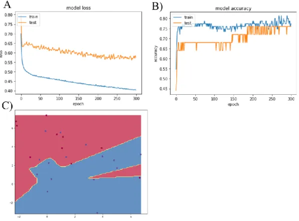
9𝑤𝜆 9_term is added to the error function for every weight (Buduma and Locascio, 2017). As lambda gets to infinity, model parameter 𝑤 will be penalized too much, so that the model will have a high bias and low variance. On the other hand, as lambda gets close to zero, the model will have a low bias, but the model will be very sensitive to the trained set and on an independent dataset which is not used to train the model, it will make more errors. This situation is called high variance. Below different models are shown with L2 regularization which have different lambda values and also a model without L2 regularization. Loss, accuracy and decision boundary graphs are plotted for the data in (Figure 1.10) with models built by using Keras (Chollet et al., 2015). All models have 2 hidden layers with 20 units in each. The number of iterations is 300. Activation functions are ReLU and sigmoid function in the output layer and optimizer is Adam.

(35)

Figure 1.11: Data are artificially made by using Sklearn make_blobs dataset (Pedregosa et al., 2011).

Figure 1.12 A&B&C: Model without L2 regularization. Figure 1.12.A) Model loss of training and testing sets Figure 1.12.B) Model accuracy of training and testing sets Training accuracy is 78.67 % and testing accuracy is 76.00 %. Figure 1.12.C) Decision

(36)

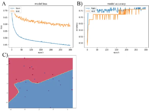
Figure 1.13.A&B&C: Model with L2 regularization 𝜆=0.01. Figure 1.13.A) Model loss of training and testing sets Figure 1.13.B) Model accuracy of training and testing sets Training accuracy is 77.33 % and testing accuracy is 76.00 %. Figure 1.13.C) Decision

Boundary

Figure 1.12C, figure 1.13C and figure 1.14C show that adding L2 regularization parameter 𝜆, prevents the overfitting problem. By adding L2 regularization, training accuracy falls a little, but the difference between training and testing accuracy becomes smaller. It is important to have similar accuracy in training set and testing set to be ensure that the model is not overfitting.

(37)

Figure 1.14.A&B&C: Model with L2 regularization 𝜆=0.1. Figure 1.14.A) Model loss of training and testing sets Figure 1.14.B) Model accuracy of training and testing sets Training accuracy is 76.00 % and testing accuracy is 76.00 %. Figure 1.14.C) Decision

Boundary

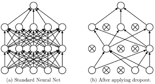
The dropout method is another regularization method. Instead of making a connection between every unit, the dropout approach makes some units inactive (Buduma and Locascio, 2017). In this method, some of the neural units in the model are rendered inactive randomly, effectively making the model independent of these units. This prevents neurons to learn excessive details about the data; thus, it can be used to prevent the overfitting problem.

(38)

Figure 1.15: Neural network with two hidden layers. (a) No dropout (b) neural network with dropout regularization (Srivastava et al., 2014)

L1 regularization is another method which can be used to prevent the overfitting problem. In L1 regularization, 𝜆|𝑤|term is added for every 𝑤 in the model (Buduma and Locascio, 2017). L2 regularization is mostly preferred and suggested regularization method instead of L1 regularization method because L1 regularization makes 𝑤 close to zero that causes the elimination of some input features. Eliminated features might be crucial features for the problem and elimination of these features might cause poor decisions (Buduma and Locascio, 2017).

1.6.4 Hyperparameters, model validation, and the bias-variance tradeoff

There are two different types of parameters in each machine learning model. One class is the trainable parameters. These are the 𝑤 and 𝑏 parameters. The algorithm tries to find the optimum values of 𝑤 and 𝑏. With correct 𝑤 and 𝑏 values, the algorithm will make correct predictions. The algorithm learns the model parameters by training.

The second class of parameters is called the hyperparameters of the model. These parameters determine how the algorithm will work. Unlike the trainable model

(39)

parameters, the algorithm does not learn the hyperparameters, as their values are set before we train the algorithm.

The learning rate 𝛼 is one of the hyperparameters. The learning rate determines the size of each step taken by the optimization algorithm at each iteration. Choosing appropriate learning rate is very important. Choosing the learning rate too small causes the optimization algorithm will converge to minimum value slowly. It will take many iterations to the algorithm will converge the global minimum value. On the other hand, choosing the learning rate too big cause another problem. The problem is that the optimization algorithm will jump to values by skipping the global minimum. Therefore, the learning rate should be selected such that the algorithm will converge the global minimum at an appropriate rate.

The number of iterations is another hyperparameter. Decreasing the number of iterations is a regulation method which prevents the overfitting by avoiding overtraining which is called the early-stop approach. On the other hand, using an insufficient number of iterations creates a high bias. Cutting the training before the algorithm reaching a desirable accuracy is called underfitting. Avoidable bias depends on the problem.

The number of hidden layers, number of units in the layers are also hyperparameters in neural networks algorithms. The number of hidden layers, number of units in the layers determine the complexity of the model. There is no rule to choose the number of layers and units. It is like a try and error process. However, researchers start with simple models and make it more complex step by step.

To train any machine learning algorithm at least two different datasets are needed. One of them is the training set and the other one is the testing set. There are different methods to divide and use data. One method is called the holdout method. The holdout method divides the data randomly into different datasets. To explore the effect of model parameters and hyperparameters dataset is divided into three datasets. These are training dataset, validation dataset and testing dataset. After the model is trained with the training dataset, another dataset is required to identify the effect of the model parameters. By

(40)

applying the same algorithm on the validation set, it is checked that the model is successful on different datasets. If the model is successful on the training set, but it fails on the validation set there are methods to modulate the model. After modifications, effect of these modifications must be tested on a different dataset to be sure the model is working properly. Testing dataset is used to prove that the model works properly not only on the validation set but also on different datasets.

K-fold cross-validation is another method of dividing the data. This method divides the data k times. Each time one of the k subsets is used as testing data and the remaining data is used to train the model. This method is the application of holdout method multiple times. K-fold cross validation method is useful when there is not enough number of data in hand. If not, enough data is divided into different sets, the model may not be trained sufficiently. This method is proper especially, for small data size.

Another important concept in machine learning algorithms is the bias-variance trade-off. When the algorithm tries to map inputs to outputs on the training set, the difference between predicted values and the real values is called bias. There is always a bias that makes the algorithm to map inputs to outputs. If the algorithm has no bias, then the model makes no connection between given features and labels on a given training set. This phenomenon is called underfitting and the model has a high bias. In this case, as the dataset is changing, there will be less difference between predicted values and the true values so-called low variance. On the other hand, if the algorithm makes the connection between every instance and every label on the training set, it has less difference between predicted and real values and it has a low bias. However, when this algorithm is tried on a different test set, it will have a significant difference between values, so-called high variance. The model will be very sensitive to specific dataset.

(41)

1.7 Implementing Neural Networks

1.7.1 Tensorflow

Tensorflow is an open source library for numerical computations created by Google in 2015. It is used for machine learning applications. Tensorflow provides functions and classes with which users can build and modify machine learning models. So, what is a tensor? Tensor is n-dimensional matrix. For instance; 3 is a rank 0 tensor, [1. , 2. , 3. ] is a rank 1, shape [3] tensor and [[1. , 2. , 3. ], [4. , 5. , 6. ]] is a rank 2 shape[2,3] tensor etc. Structure of mathematical functions are described by computation graph. To work Tensorflow, first the graph is defined and then this computation graph is run. Nodes represent computations and edges represent link between nodes in the computation graph. The figure below shows a simple computation graph. Circles represent nodes that are operations in the computation graph and arrows represent edges. Nodes a and b take input values which are 3 and 5 in this case and direct them to nodes c and d which are multiplication and addition operations. Last node e takes values from c and d nodes and computes addition. In this example node e is directly dependent on c and d and it is indirectly dependent on a and b. This means that e needs values from c and d to compute operation, but values from a and b are not directly fed to e (Abrahams et al., 2016). Dependency is an important concept because making wrong dependencies cause infinite loops. If the node e is dependent on c and c is dependent on e, then the algorithm will never give a solution because each node will wait for the answer of the other node.

(42)

There are different types of objects in the Tensorflow that are constants, variables, and placeholders. Constants have values specified when they are created and these values cannot be changed in the future operations. Constants are immutable. On the other hand, variables contain mutable values; means that values can be changed. Placeholders do not have their values specified when created. They hold the place for a Tensor that will be fed at running the session (Abrahams et al., 2016).

Different machine learning algorithms and gradient descent functions can be used to build different models. Tensorflow made is easy to build complex models. There are different operations in Tensorflow. One of them is mathematical operations such as multiplication, summation as described above. There are also different operations to build a model. One of them is matrix operations such as Matmul, which is short for matrix multiplication, Matrix Inverse, which takes the inverse of the matrix. Matrix operations are very important because features and samples are stored as vectors. For different machine learning algorithms, Tensorflow provides different building blocks. There are linear regression, logistic regression, softmax activation function, artificial neural networks. In Tensorflow different optimizers and model parameters can be used to minimize error in a model. The algorithm is chosen based on the problem. Tensorflow is very useful for deep learning because it stores mathematical computations in the nodes. In the neural networks algorithm, during backward propagation partial derivatives are taken with chain rule. Even the values are not fed, defining the mathematical computation is enough to prepare derivative of the computation. Storing derivatives of the mathematical computations with Tensorflow makes neural network algorithms work fast.

1.7.2 Keras

There are other libraries that can be used for deep learning. One of them is Keras. Keras is a high-level neural networks API which is written in Python and it can run on Tensorflow or Theano (Chollet et al., 2015). There are Keras Sequential Model and the Functional API. Sequential model needs so little user operation to build and run a model. The user can control the number of layers, number of units in layers, type of activation

(43)

function and other hyperparameters to build a deep learning model in Keras. Activation function can be ReLU, tanh or sigmoid functions. in the hidden layers. In the output layer, softmax activation function is used for multi-label classification problems. In the output layer, sigmoid function can be used for binary classification problems. Different loss functions and different optimizers can be used to minimize the loss. Keras has gradient descent and stochastic descent algorithms. Keras provides lots of options to the user to build, train and optimize a model. It is a user-friendly environment.

(44)

2. MATERIALS AND METHODS

We applied different machine learning algorithms to four different datasets. These datasets are taken from University of California Irvine machine learning repository web site.

All problems are supervised machine learning classification problems. Type of classification depends on the problem. There are binary classification problems and multi-class multi-classification problems as described in the dataset explanations in sections 2.1, 2.2, 2.3, 2.4.

Jupyter notebook is an open source tool that is used for data science and machine learning. It provides Python environment along with markdown support. In this environment, users can develop scientific projects by importing libraries such as Pandas, NumPy, Tensorflow, and Keras. One can create new Jupyter notebook documents for storing different projects. Therefore, we created multiple Jupyter notebook documents for each dataset in order to use Pandas, NumPy, Tensorflow, and Keras.

Moreover, we used matplotlib library to visualize the datasets and the results. In particular, for the results section, we heavily used visualization of the accuracy, the cost function, and the confusion matrix.

For each problem, different supervised machine learning algorithms are applied. Based on the accuracy results, models are modified. If the applied algorithm does not give the desired result, then different algorithms are applied.

(45)

2.1 The Yeast Dataset

The yeast dataset is taken from UCI machine learning repository (Murphy and Aha, 1996). The dataset has 1484 instances, 8 attributes and 10 classes (Horton and Nakai, 1996). Classes are the localization sites of the proteins in the yeast cell. These proteins are categorized based on the localization sites as follows; cytoskeletal, nuclear, vacuolar, mitochondrial, peroxisomal, the cell wall, the lumen of the endoplasmic reticulum, membrane proteins with a cleaved signal, membrane proteins with an uncleared signal and membrane proteins with no N-terminal signal (Horton and Nakai, 1996).

2.2 The Gene Expression Cancer RNA-Seq Dataset

This dataset contains gene expressions of patients who have different types of tumors. Cancer types are breast invasive carcinoma, kidney renal clear cell carcinoma, colon adenocarcinoma, lung adenocarcinoma and prostate adenocarcinoma (Weinstein et al., 2013). It is taken from UCI machine learning repository.

2.3 The Breast Cancer Wisconsin (Diagnostic) Dataset

This dataset is taken from UCI machine learning repository. The dataset contains 32 real-valued features computed from a digitized image of a fine needle aspirate of a breast mass (Street et. al., 2009). The problem is making classification of two types of breast cancer that are malignant and benign.

2.4 The Epileptic Seizure Recognition Dataset

This dataset is taken from UCI machine learning repository. The dataset has 178 features, which are brain activity of patients for a second, and brain activity is recorded for 23 seconds in total. The brain activity of patients is recorded with EEG. The problem is taken as a binary classification problem. We determine if the patient has an epileptic seizure or not (Andrzejak et. al., 2001).

(46)

3. RESULTS

3.1 Application of The Softmax Classification Algorithm and Logistic Regression

Before applying neural networks algorithm to the problems, simple softmax classification algorithm is applied to the problems and the accuracies of the problems are determined. By using Tensorflow library, different sessions are prepared for each problem. First of all, the dataset is uploaded and the input values are determined as matrix x and the output labels are matrix y. Categorical output labels are converted to numerical values by using OneHotEncoder from sklearn preprocessing library (Pedregosa et al., 2011). One hot encoder converts the categorical output feature for an example to a vector such that 1 for the true class of the example and 0 for the other classes. The dataset is split to the train and test datasets by using sklearn train test split (Pedregosa et al., 2011). Then, feature normalization is done for the train and test sets. Mean values and standard deviation values for the train and test sets are calculated by using the input features. The mean value is subtracted from each input value and divided to the standard deviation value. After the train set, test set preparation is completed, placeholders for the datasets as X and Y and variables W and b for weight and bias terms are written. Softmax cross entropy in Tensorflow (tf.nn. softmax_cross_entropy_with_logits) is used as the cost function. Gradient descent optimizer of Tensorflow is used to optimize the algorithms (Abadi et al., 2015). The learning rate and the number of iterations are given during running the session. Firstly, to train the model, the training set is fed to the placeholders X and Y. After the training is completed, the accuracy for the training is calculated. Finally, the accuracy for the test set is calculated as the testing set is fed to the placeholders X and Y. The learning rate and the number of iterations that are the hyperparameters are selected for each problem separately. The learning rates are determined such that the gradient

(47)

descent algorithm converges to the minimum with a proper rate. The number of iterations is determined by the decrease rate of the cost function. After a certain number of iterations for a problem, we see that the cost does not decrease and the accuracy does not increase, so we did not continue to train the model. In addition, the number of iterations can be used as regularization because overtraining the algorithm causes the overfitting problem. By dividing the datasets into the training and testing sets, we want to prove that applied algorithm is not overfitting. The accuracy of the training data and the accuracy of the testing data are very similar. It shows that we do not have high variance. The model gives similar results on an independent set which is not used in the training. When there is an overfitting problem, the training accuracy is much higher than the testing accuracy. Results of the problems show that there is no overfitting.

Table 3.1: The training and the testing accuracies of datasets with the softmax classification algorithm Determination of protein locations in yeast Determination of cancer type based on gene expression Determination of two breast cancer types Determination of Epileptic Seizure Training Accuracy 59.22 % 99.50 % 91.65 % 52.83 % Testing Accuracy 58.59 % 99.00 % 91.23 % 52.35 %

(48)

Figure 3.1.A&B: The softmax classification approach on the yeast dataset Figure 3.1.A) Gradient descent plot Figure 3.1.B) Training and testing errors vs. number of

iterations plot. The training accuracy is 59.22% and the testing accuracy is 58.59%

Figure 3.2.A&B: The softmax classification approach on the breast cancer dataset Figure 3.2.A) Gradient descent plot Figure 3.2.B) Training and testing errors vs. number

(49)

Figure 3.3.A&B: The softmax classification approach on the determination of cancer type based on the gene expression dataset 3.3.A) Gradient descent plot Figure 3.3.B) Training and testing errors vs. the number of iterations plot. The training accuracy is

99.50 % and the testing accuracy is 99.00 %.

Figure 3.4.A&B: The softmax classification approach on the epileptic seizure recognition dataset 3.4.A) Gradient descent plot Figure 3.4.B) Training and testing errors vs. number of iterations plot. The training accuracy is 52.83 % and the testing

accuracy is 52.35 %.

The softmax classification algorithm is found to be successful for two problems. These problems are the determination of two breast cancer types and the determination of the

(50)

cancer type based on the gene expression. The accuracy of the training set is 91.65 % and the accuracy of the testing set is 91.23 % for the determination of two breast cancer types problem. For the determination of the cancer type based on the gene expression problem, the training set accuracy is 99.5 % and the testing set accuracy is 99.0 %. Neural network algorithm is not applied to these problems because the softmax classification algorithm is already highly successful. We can say that the data of these problems are linearly separable because the softmax classification algorithm separates any two classes with a linear decision boundary. On the other hand, the softmax classification algorithm did not work well on the determination of the protein locations in yeast and the determination of epileptic seizure problems. It indicates that these datasets are not linearly separable. To obtain better results on these complex problems, we applied nonlinear feedforward neural networks algorithm.

3.2 Determination of The Protein Locations in Yeast

The yeast dataset is divided into the training and testing sets by using sklearn train test split method (Pedregosa et al., 2011).

The number of neighbors which is represented as K (note that it is not related to k described in k-fold cross-validation method) is taken from 4 to 50. Scores of each K value is calculated.

Figure 3.5: Misclassification error vs. number of neighbors

(51)

3.2.1 Classification using the neural networks approach

Neural networks approach is first applied to the determination of the protein locations in the yeast dataset. All models are built by using Keras library (Chollet et al., 2015) In all models, activation functions in the hidden layers are ReLU activation function. In the output layer, the activation function is the softmax activation function because the problem is a multi-class classification problem. Adam optimizer is used and 500 iterations are made in each model. The learning rate is taken as 0.005. Categorical cross-entropy is used as the cost function. The dataset is divided into the training, validation and testing sets by using sklearn train test split (Pedregosa et al.,2011). In all models, the training, validation and, testing datasets are same to compare and modify the models.

Table 3.2: Architecture of neural network models

In the first model, the number of hidden layers is taken as 3. In each hidden layer, there are 10 units. Regularization methods are not applied in the first model. The training accuracy is 67.19 % and the validation accuracy is 57.58 %. To increase the accuracy,

(52)

one more hidden layer is added while the number of units and the other parameters are same. The training and validation accuracies are checked. The training accuracy is 68.88 % and the validation accuracy is 54.55 % in model 2. Adding more hidden layers does not increase the validation accuracy.

Figure 3.6.A&B: Model 1. Figure 3.6.A) Model loss Figure 3.6.B) Model accuracy. The training accuracy is 67.19 % and validation accuracy is 57.58 %.

Figure 3.7.A&B: Model 2. Figure 3.7.A) Model loss Figure 3.7.B) Model accuracy. The training accuracy is 68.88 % and the validation accuracy is 54.55 %.

(53)

In model 3, the number of units in the hidden layers is increased to 12 while other parameters are kept same as the model 1. The training accuracy is 69.21 % and the validation accuracy is 54.88 %. The validation accuracy of the first model is the highest. However, in the first model, there is a high variance. To regulate the high variance regularization methods are applied. Firstly, L2 regularization method is applied by taking 𝜆 0.001. The validation accuracy increased from 57.58 % to 58.25 % in model 4. However, there is still a high variance, so 𝜆 value is increased to 0.01 in model 5. The training accuracy becomes 68.32 % and the validation accuracy becomes 58.59 % in model 5. In model 6, 𝜆 is taken as 0.1. The training accuracy is 64.27 % and the

validation accuracy is 60.27 %. In the model 7, 𝜆 is taken as 1. The training accuracy is 61.69 % and the validation accuracy is 57.91 %.

Figure 3.8A&B: Model 3. Figure 3.8.A) Model loss Figure 3.8.B) Model accuracy. The training accuracy is 69.21 % and the validation accuracy is 54.88 %.

(54)

Figure 3.9.A&B: Model 4. Figure 3.9.A) Model loss Figure 3.9.B) Model accuracy. The training accuracy is 68.88 % and the validation accuracy is 58.25 %

(55)

Figure 3.11.A&B: Model 6. Figure 3.11.A) Model loss Figure 3.11.B) Model accuracy. The training accuracy is 64.27 % and the validation accuracy is 60.27 %

(56)

Another regularization method is applied while other parameters are same to see if the dropout regularization method works better than the L2 regularization method or not. In the eighth and ninth models, the dropout regularization method is applied, but this method does not provide a better solution to the high variance problem than the L2 regularization method.

Figure 3.13.A&B: Model 8. Figure 3.13.A) Model loss Figure 3.13.B) Model accuracy. The training accuracy is 61.12 % and the validation accuracy is 57.58 %

(57)

Figure 3.14.A&B: Model 9. Figure 3.14.A) Model loss Figure 3.14.B) Model accuracy. The training accuracy is 58.76 % and the validation accuracy is 54.88 %

In the last step, model 10, 𝜆 value is 0.5; the training and validation accuracies are 61.69 % and 61.62 % respectively. Similar training and validation accuracies ensure that there is no overfitting anymore.

After the overfitting problem is solved, we wanted to check the effect of the hyperparameters. The hyperparameters are chosen based on the accuracy of the validation set. We wanted to prove that the model does not work well only on the validation set. To prove this, we run our model on a different dataset that is the testing set. The testing accuracy of Model 10 is 61.28 %. Accuracies of both training, validation, and testing sets are quite similar to each other. It proves that the model is working the same on different datasets.

Figure 3.15.A&B: Model 10. Figure 3.15.A) Model loss Figure 3.15.B) Model accuracy. The training accuracy is 61.69 % and the validation accuracy is 61.62 %. The

(58)

Even though the model does not have a high variance, it does not perform well. To check where the algorithm is making wrong predictions, we plotted confusion matrix. As we can see in the confusion matrix, the model makes wrong predictions especially on classes in which the number of available samples is small. The model predicts the classes of the proteins which are the proteins located in the endoplasmic reticulum and in the vacuole all wrong. The small number of available samples in these locations possibly causes it. There are only 5 samples that are located in the endoplasmic reticulum and 30 samples in the vacuole.

Figure 3.16: Confusion matrix for the 10th _{model on the yeast dataset}

We have small number of examples in this dataset. Especially, some classes have only a few numbers of instances. Dividing the dataset into the training, validation and testing sets cause the insufficient number of data in the training. To avoid this problem and use as much as data in the training part to increase the accuracy, we applied the cross-validation method.

(59)

By using the parameters of model 10, cross-validation is performed. The dataset is trained in 10 groups. The mean of the accuracy is 52.82 % and the standard deviation is 4.15 %. The best accuracy of the cross-validation method is calculated as 59.73 %. The high standard deviation is caused by the irregular dataset.

Table 3.3: Accuracy results by using the cross-validation method and 10th_method

parameters Partition _Accuracy 0 59.73 % 1 50.34 % 2 55.70 % 3 58.39 % 4 52.70 % 5 47.30 % 6 52.03 % 7 52.70 % 8 53.38 % 9 45.95 %

To obtain better results in this problem, we need much more training samples. It shows that the size of the dataset is as important as the model. The softmax classification algorithm gives 58.59 % accuracy and the neural networks algorithm gives 61.28 % accuracy. The neural networks algorithm is much more complex than the softmax classification algorithm. The softmax classification algorithm separates any two classes linearly. The neural networks algorithm is used to classify linearly inseparable data. In this problem, the neural networks algorithm increased the accuracy by almost 3 %. We