Supervisory-plus-regulatory control design for efficient operation of industrial furnaces

Received Date : 21.02.2004 Accepted Date: 15.06.2004

SUPERVISORY-PLUS-REGULATORY CONTROL DESIGN FOR

EFFICIENT OPERATION OF INDUSTRIAL FURNACES

Zhivko A. ICEV

*

Jun ZHAO

**

Mile J. STANKOVSKI

*

Tatyana D. KOLEMISEVSKA-GUGULOVSKA

*

Georgi M. DIMIROVSKI

***

* Institute of ASE-FEE, SS Cyril and Methodius University, Skopje, Republic of Macedonia {z_icev, milestk, tanjakg}@ etf.ukim.edu.mk

** Institute of Control Science, Northeatern University, Shenyang, Liaoning, P.R. of China zdongbo @ sy-public.ln.cinfo.net

*** Department of Computer Eng., Dogus University, 34722 – Kadikoy / Istanbul, Turkey gdimirovski @ dogus.edu.tr

ABSTRACT

A two-level system engineering design approach to integrated control and supervision of industrial multi-zone furnaces has been elaborated and tested. The application case study is the three-zone 25 MW RZS furnace plant at Skopje Steelworks. The integrated control and supervision design is based on combined use of general predictive control optimization of set-points and steady-state decoupling, at the upper level, and classical two-term laws with stady-state decouling, at the executive control level. This design technique exploits the intrinsic stability of thermal processes and makes use of constrained optimization, standard non-parametric time-domain process models, identified under operating conditions, using truncated k-time sequence matrices, controlled autoregressive moving average models. Digital implementations are sought within standard computer process control platform for practical engineering and maintenance reasons.

Keywords: Complex time-delay processes; generalized predictive control; integrated control and supervision; optimization; regulatory control..

1. INTRODUCTION

My own conclusion is that engineering is an art rather than a science, and by saying this I imply a higher, not a lower status – Howard H.

Rosenbrock

Systems engineering design based on integrated control and supervision by using optimization methods by itself is a compromising quest to meet the main objective criteria while satisfying unavoidable engineering constraints and requirements. Once again the obove cited words of Professor Rosenbrock [1] appeared to be

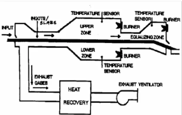
valuable guidance in designing complex control systems. In addition, systems philosophy framework, in which mutal impact have the original real-world systems and their conceptual models and mathematical representations [1], should be adopted along the thinking that dynamical processes in the real world (below the speed of light) constitute a unique non-separable inter-play of the three fundamental natural quantities of energy, matter and information [2]. Moreover, energy and matter are information carriers, but solely information has the impact capacity as to modulate and direct energy and matter transformation with the unavoidable constraints. And the system engineering design for improved, energy saving, operation of large industrial furnaces by using a two-level, integrated supervision and control system, reported in here, is focused on such an approach [3] precisely by making use of known scientific results in systems and control theory [4], [5], [6]. The case study problem solved is a real-world, 28/25 MW, three-zone, pusher furnace (Figure 1.1) at Skopje Steeilworks [7].

Process designs and plant constructions of industrial furnaces have been subject to both scientific and technological research for long time [8]. Nonetheless, their control and supervision have never seized to topics of extensive research due to the complexity of energy conversion and transfer process in high-power, multi-zone furnaces. From this point of view, these thermal processes have been summarized and operationally characterized as: operating regimes of different-load as well as start-up and shut-dawn; convex control (or steady-state) input-output characteristics at operating points; slow and non-linear, but locally linearizable, overall dynamics; varying time-delays; problematic sensor distribution; delicate sensor-actuator collocation; under stabilized pressure the main controlled variables are temperatures and controlling variables are energy (fuel/gases) supply/release [9]. Real-world industrial high-power furnaces in steel mills are operated with gas/oil fuel in difficult field environment [7], [9], which requires considerable maintenance support. Main disturbances come along with the line-speed and heated mass flow as well as the hot gas and air flows inside the reheat processing space. Also, varying dimensions and grades of slabs in lower-grade steel processing (as at Skopje Steelworks) act as disturbances too (Figure 1.2).

Fig. 1.1 Construction schematic of the three-zone

28/25 MW pusher furnace RZS at Skopje Steelworks

Fig. 1.2 An illustration of input-output signal

flow paths of furnace thermal process also indicating the main input-output control characteristics and dynamics

The overall control task is to drive the process to the desired thermodynamic equilibrium and to regulate it there as well as to maintain the temperature profile through the plant. Hence, for such plant systems, two-or three-level control system architecture and hybrid controls have to be employed [10], [11], [12]. Through appropriate system analysis and within such control system architecture, the goals and the margins of controlled processes may be mapped onto formal models of inputs to the algorithms of the supervisory (upper) control and the regulation (lower) control levels in terms of a family of primitives and sets of rules along with some additional model data for deign and tuning. From industrial practice of slab pusher furnaces in steel mills, it is well-known that the temperature regulatory level is capable to maintain the process variables close enough to the command set-points [7]. This performance is

further enhanced if a steady-decoupling design is used for setting up the steady-state operating point. Separate executive controls that stabilize the pressure and ensure the general operating conditions are maintained, when the gas-burners are properly actuated. The operational pace is imposed by production scheduling of the slab rolling plant that follows the reheat furnace (e.g., see [10], [12]).

However the economic reasons, in particular the one on energy cost (fuel consumption) per product unit, and operational technical restrictions make it necessary to optimize plant operations one way or another [13], [14], [15]. Due to the need of both set-point and optimization control tasks, practice and research insofar have demonstrated that there are three alternatives to resolve the optimization problem: (i) an optimally designed controller to replace the regulatory level in performing both tasks (e.g., see [15]; (ii) an optimization expert system is combined with executive regulatory controls to perform both tasks (e.g. see [10]); (iii) a supervisory set-point optimization control is added while retaining the classical regulatory level (e.g., see [16], [17] and the works referenced in the next section). Practice has demonstrated that the first alternative hardly leads to feasible implementation designs, and the second one requires a costly development of an appropriate heuristic expert system to perform the optimization at the supervisory control level. To the best of our knowledge (e.g., see [7], [12], [18]), we have found that the third alternative is worth exploring for practical cost-effectiveness and maintenance reasons, and the findings are reported in here.

The rest of this paper is written as follows. In the next Section 2, an overview discussion on the background research is given. The subsequent Section 3 gives a brief presentation of the methodology approach and solving techniques applied. In Section 4, first an outline of the RZS 3-zone furnace and the features of its operational dynamics and steady states as revealed by series of step and PRBS identification tests at typical operational loads (e.g., 30%, 60% and 80%) are given. And thereafter the more important results of the control design and test results along with a relevant discussion are presented. Conclusions and references are given thereafter.

2. ON THE BACKGROUND

RESEARCH

In the literature, in the first place, there may be found in a number of studies that deal with set-point optimization based on steady-state models. Ellis and co-authors have presented their design in [19] for economic optimization of a fluidized catalytic cracking unit. There the regulatory level comprises a constrained non-linear controller the set-points of which are computed by the optimization level whereby the parameters of the steady-state models are adapted on-line. Also based on the use of steady-state models, Becerra and co-authors [20] have proposed a multi-objective predictive formulation that includes both economic and regulatory objectives. Zheng and co-authors [21] have reported a hierarchical control strategy in order to maximize the profit of a chemical plant. They used the steady-state process models to determine the set-points so that an economic objective function is optimized. Munoz and Cipriano [22] have elaborated an economic control strategy for a mineral processing plant. Their strategy uses a regulatory level based on multi-variable predictive controllers and a global economic optimizer in order to determine the set-points of the predictive controllers. In their work, they have considered non-linear steady-state models of the grinding process and dynamic models of the flotation process given the pragmatic observation that time constants of the flotation are smaller than the ones of the grinding processes.

A rather interesting approach has been proposed by De Prada and Valentin [23]. In order to determine optimized level set-points for the regulatory of a sugar processing plant, they have proposed a predictive control strategy based on an economic index optimization. They obtained the optimal set-points at the supervisory level by optimizing a multi-variable objective function. And the regulatory level is solved by using the GPC algorithm while also including constraints on the amplitude and on the slew rate of executive (manipulated) variables and the limits on controlled variables. The same predictors and constraints as for the regulatory level GPC controllers are used to solve the optimization problem. The optimization variables correspond to the increments of the executive variables. The optimal set-points are defined as the values of the controlled variables at time instant

t

+

N

_y,

which corresponds to the optimal increments of the obtained executive variables. This procedure is repeated for each sampling instant, thus resulting in dynamically optimal set-points. Indeed, model-based predictive control algorithms have been successfully applied to many different industrial processes, since the operational and economical criteria may be incorporated using an objective function to calculate the control action [24], [25], [26], [27]. Moreover, in their very essence, these control strategies rely on the optimization of the future process behavior with respect to the future values of the executive control (process manipulated variables) and their extension to use non-linear process models is motivated by improved quality of the prediction of inputs and outputs [28]. This way, non-linear predictive controls are derived albeit these do not have a specific control strategy of their own. Rather these utilize the one of the methods associated with linear predictive control that is optimization of an objective function, possibly with constraints [29].

Tsang and Clarke [5] have derived a GPC algorithm in which the constraints on executive control variables for two sampling instants of the control horizon were also incorporated. Subsequently, Demircioglu and Clarke [6] have presented a continuous time GPC controller design based on state space models with constraints in which system stability was also ensured. A similar problem was solved by Camacho [30] where constraints on both executive control and controlled variables were incorporated. In this case, to reduce the computing effort, the solution was obtained by transforming the quadratic optimization problem into a linear optimization problem. Along these consideration lines, Camaco and Burdons [31] have presented as a benchmark a simple furnace heat transfer and the respective GPC designs, which is of direct importance for the case of industrial furnaces as the one in our case study problem [32]. Cipriano and Ramos [33] have developed a fuzzy model based predictive controller for the mineral flotation plant as in Munoz and Cipriano [22].

Also, there are published papers in the literature reporting on optimization designs regarding the supervisory level that are based on dynamic models. In works by Yang and Lu [10], [13] there have been reported both the development

of an appropriate dynamic process model for the supervisory optimization level and the expert system based supervisory-plus regulatory control design, where the expert system employs a heuristic rule base that they have developed. Subsequently, Lu and Markward [34] have developed another integrated supervision and control system design, employing neural network models, for a hot-deep coating-line of steel strips which also achieves the set-point optimization. In the work for a thermal power plant simulator by Katebi and Johnson [35], there is described a decentralized control strategy based on the optimization of a particular objective function as GPC algorithms by using a state space representation model. It should be noted, to solve the optimization problem, they considered the executive variables as the optimization variables and, from these variables, the optimal set-points are obtained using a procedure similar to the one used by De Prada and Valentin [23]. However, a Kalman filter has been employed to estimate the state vector and this is what complicates the overall system when practical system engineering designs are sought. For if a Kalman filter is to be employed, then the technique due to Yang and Lu [10] (implemented system engineering design to real-world plants) is superior for real-world applications, in addition to other advantages.

Bemporad and co-authors [36], Mosca and Zhang [37], and Angeli and Mosca [38] have also used a state-space representation model. Based upon assumption that a desired reference trajectory is usually available, they have proposed a reference governor at the supervisory level. The main goal was to satisfy certain given constraints. The objective function is defined in terms of the error to the reference trajectory and minimized, and the algorithms developed. The main idea of our approach is to improve furnace operation so that some more ‘calm’ regulatory controls are obtained via slightly time-varying set-points to the regulatory level, which in turn are obtained by using general predictive control concepts and constrained optimization. Another objective is to employ rather simple and math-analytical models that lead to a feasible two-level control strategy. An appropriate objective function is to be minimized for this purpose similarly as in works [22], [23], [30], [33]. This objective function may represent

several relevant parameters such as operational costs, control energy consumption and even other criteria, including also regulatory objectives of integrated square of the tracking error. It is a fairly general yet flexible objective function and was adopted it in our research too. In general, from the viewpoint of industrial process control [10], [16], [32], the investigated problem of integrated supervisory-plus-regulatory control for industrial multi-zone pusher-type furnaces as an optimization oriented system engineering problem may be formulated in terms as presented bellow. Let some model providing for either real-time estimation or predication of internal process information to be used as an available resource for supervisory optimization control. Then the problem reduces to selecting a vector of admissible controls

=

)

(k

U

[

u

₁

(

k

)

.

.

.

u

_r

(

k

)

]

T, within some time horizon

T

_H, such that some performance index

∑

− = =

=

1 0

))

(

),

(

(

H T k k

k

Y

k

U

unction

ObjectiveF

J

(2.1) is minimized subject to

)

),

(

),

(

(

)

1

(

k

f

Y

k

U

k

P

Y

+

=

,

Y

(

0

)

=

Y

₀, (2.2) Y

SP

Y

∈

,

U

∈

SP

_U,

P

∈

Ω

_P. (2.3) In this formulation,

U

represents a control vector for process optimization, which could be reference set-points to local lower control level,

Y

represents a vector of feasible controlled variables, and

P

represents a vector of real-valued parameters and possibly some qualitative constraints within some pre-specified domain. In principle, the formulated optimization problem [39] can be solved either directly (e.g., linear case with quadratic criterion) or indirectly through numerical computations (e.g., non-linear case with Kuhn-Tucker conditions), or by an iterative heuristic search (e.g, as in [14]), or by math-analytical nonlinear optimal control synthesis (e.g., as in [40]).

3. SOLVING METHODOLOGY FOR

SUPERVISORY-PLUS-REGULATORY CONTROL

DESIGN

The adopted solving approach to the problem of concern is as follows: firstly, a good design of the regulatory level that will provide executive controls (vector

u

) to the supervisory level for controlling measured process variables (vector

y

) while compensating the non-measured varying disturbances (vector

e

); and secondly, an optimized design (via minimizing a suitable performance objective function

J

) of the supervisory level to determine the optimal set-points (vector

r

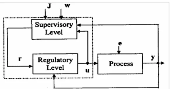
) so that the relevant constraints accounted for into the performance index are satisfied (see Figure 1). In principle, should it be available, an external reference trajectory (vector

w

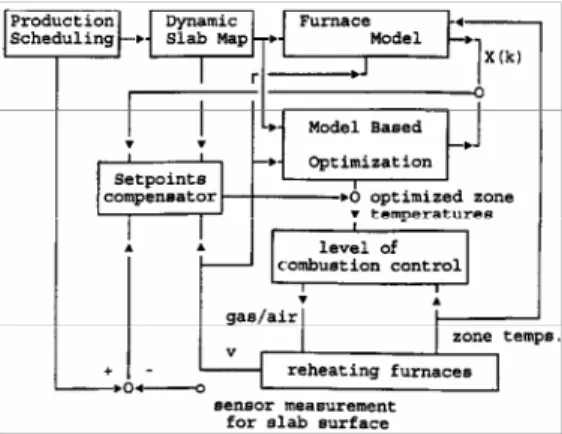
; not needed in our case study) can be included into the performance index. Hence, the supervisory level dynamically optimizes a general objective function subject to equality and inequality constraints, the overall control strategy is a hybrid one and the overall system will be stable with the conditions satisfied. From an overall system engineering point of view, the resulting optimum may not be global but rather a local one because the regulatory level confines systems transients locally. Yet this solving approach resolves the posed problem.

Figure 1. The overall architecture of a

two-level supervisory-plus-regulatory control system.

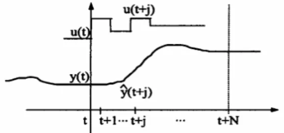
This problem, when constraints are accounted for and/or non-linear models are used, can be solved by numerical algorithms following the third conceptual alternative (see Section 1) and hints drawn from the theory of model based predictive control [29], [31], 41]. As known from the literature [4]-[6] (also see Figure 2), the main

methodological steps in designing model based predictive controls are the following:

- The future outputs of controlled variables, for a determined horizon

N

_y, are predicted at each time instant

t

using some model of the process to be controlled. The output predictions

)

(

t

j

y

+

conceptually depend on the known values of process variables up to time instant

t

(the past history) and on the future control signals

u

(

t

+

j

)

which are to be calculated.

Figure 2. An illustration of the main idea of the

model based predictive control theory (Clarke and co-authors, 1987)

- The future control signals

u

(

t

+

j

)

are calculated by optimizing a predefined objective function (criterion of performance index) in order to keep the process as close as possible some desired reference trajectory. To the best of our knowledge, rightly in most cases and the criterion is defined in terms of some quadratic form, e.g. a quadratic function of the errors between the predicted output signal and the predicted reference trajectory and of the control effort if controlling variables are to be optimized as well as in our case study.

- The control signal

u

(

t

)

is executed on the actual process, and at the next sampling instant

1

+

t

the values of all the controlled variables until then and of all the executive control variables until time

t

are known.

- The concept of the receding horizon is used so that only the first control action from the assumed control horizon is applied at the present time instant and kept until the next one. Then, both the prediction and control horizons are moved one step into the future, and the procedure is repeated at the next time instant. It should be noted that a suitable process model is crucial and it has to be adopted (developed or experimentally identified), and only then model based predictive control derived.

In the reality, steel mill industrial processes are characterized by non-stationary stochastic disturbances by and large of Gaussian nature, and so is the case with Skopje Steelworks. Therefore, as argued by Clarke in his works (e.g., see [4], [5], [6]), the appropriate choice is a model of the class controlled autoregressive and moving-average process. Its general representation for the single-input-single-output case and constant sampling period (the equidistant time-shifting intervals) is given as follows:

∆

+

=

− −

₎

₍

₎

₍

₎

₍

₎

₍

₎

_/

(

_q

1

_y

_t

_B

_q

1

_u

_t

_e

_t

A

with

q

−1 the backward shift operator (that is, e.g.

q

−1

v

(

t

)

=

v

(

t

−

1

)

) and

∆

=

1

−

q

−1, where

e

(

t

)

represents a zero mean white noise, and na na

q

a

q

a

q

A

−

₌

₊

−1

₊

_⋅

_⋅⋅

₊

− 1 1

₎

₁

(

, nb nb

q

b

q

b

q

B

−

=

+

−1

+

⋅

⋅⋅

+

− 1 1

₎

₁

(

the appropriate polynomials in

q

−1 (computer process control implementation).

Thus, given a design of the regulatory control level implying fixed control algorithms, the respective model for the supervisory level may be represented by the following expression:

)

(

)

(

)

(

)

(

)

(

)

(

_q

1

_u

_t

_B

_q

1

_r

_t

_B

_q

1

_y

_t

A

_rc −

=

_rc −

+

_ry − (3.1) with nra nrc rc rc

q

a

q

a

q

A

−

=

+

−1

+

⋅

⋅⋅

+

− 1 1

₎

₁

(

, (3.1 a) nrb nrc rc rc

q

b

q

b

q

B

−

₌

₊

−1

₊

_⋅

_⋅⋅

₊

− 1 1

₎

₁

(

, (3.1 b) nry nry ry ry ry

q

b

b

q

b

q

B

−

₌

₊

−1

₊

_⋅

_⋅⋅

₊

− 1 0 1

₎

(

. (3.1 c) The objective function, representing the optimization criterion at the supervisory level, has to account for accounts for the dynamical behavior over the prediction horizons. The objective function class used in [5], [22], [23],

[30], [31] is well justified with respect to both controlled and control variables, and was adopted in our work too. That objective function may represent different optimization goals at the supervisory level. In particular, it may represent the operational costs or the profit of a plant, or the process energy consumption, and also integral-square criteria for the regulatory level can be accommodated. It should be noted that, in practice, care has to be taken the objective function to account for the essential performance measuring terms while kept as simple as possible for pragmatic reasons. In its scalar form, the objective function adopted may be written dawn as given bellow:

∑

∑

= =

+

−

+

Ψ

+

+

Ψ

=

y Nu i i u N j j y

y

t

j

u

t

i

J

1 2 1 2

₍

₎

_ˆ

₍

₁

₎

ˆ

∑∑

= =

+

−

+

+

Ψ

+

Ny u j N i ji yu

y

t

j

u

t

i

1 1

)

1

(

)

(

ˆ

∑

= ∆

+

−

+

∆

Ψ

+

Nu i j u

u

t

i

1 2

₍

₁

₎

∑

=

+

+

u N i j y

y

t

j

1

)

(

ˆ

ξ

∑

∑

= ∆ =

−

+

∆

+

−

+

+

u Nu i i u N i i u

u

t

i

u

t

i

1 1

)

1

(

)

1

(

ξ

ξ

. (3.2) In (3.2 ) the individual quantities denote:

N

_u and

N

_y are prediction horizons;

y

(

t

+

j

)

are the j-step ahead predictions of the controlled variables based on data up to time

t

;

)

1

(

t

+ i

−

u

are the executive controls (manipulated variables); and

∆

u

(

t

+

i

−

1

)

are the increments of the executive controls;

Ψ

_yj,

i u

Ψ

,

Ψ

_yuji,

Ψ

_∆i_u and

ξ

_yj,

ξ

_ui,

ξ

_∆i_u are suitable weighting sequence matrices and vectors. (Notice, if known in advance, an external reference trajectory

w

=

w

(t

)

can also be included into the objective function as appropriate.)

In normal furnace operation, besides the limits imposed on the controlled process variables, practical operating characteristics of actuators also impose constraints on the amplitude and the slew rate of the manipulated process variables.

Hence, the following constraints are to be observed:

- amplitude limits on the

j

=

1

,

...,

N

_y controlled process variables,

max

min

y

ˆ

(

t

j

)

y

y

≤

+

≤

; (3.3) - amplitude limits on the

i

=

1

,

...,

N

_u executive control (manipulated) variables

max

min

u

(

t

i

1

)

u

u

≤

+

−

≤

; (3.4) - increment constraints on the

i

=

1

,

...,

N

_u executive control (manipulated) variables,

max

min

u

(

t

i

1

)

u

u

≤

∆

+

−

≤

∆

∆

; (3.5)

Notice that the constraints are imposed on

)

(

ˆ

t

j

y

+

, that is the

j

−

th

step ahead prediction of the controlled process variables. The control action is to be obtained by minimizing the objective function (3.2) under the equality constraints (3.1) and the inequality constraints (3.3)-(3.5). For this purpose, prediction of the control variables is calculated as a function of past values of the input controls and measured outputs and of a horizon future control actions.

As known from the literature [39], an explicit analytical solution to this optimization problem can be obtained directly if the criterion is quadratic, the model is linear, and there are no constraints. This case is of a more academic nature, because in practice there unavoidable constraints for many technological reasons [32], and so is the industrial furnace operation considered. Thus only a numerical optimization indirect solution can be sought via introducing a Lagrangean function, typically, using Kuhn-Tucker conditions (Luneberger, 1984). In practice, with regard to computational effort involved, the optimization variables are reduced to:

y

ˆ

(

t

+

1

)

, …,

y

ˆ

(

t

+

N

_y

)

;

u

(t

)

,

u

(

t

+

1

)

, …,

u

(

t

+

N

_u

)

,

r

(

t

)

,

r

(

t

+

1

)

, …,

)

(

t

N

_y

r

+

. In turn, the inequality are slightly reduced. In addition, on the grounds of the process model for predictive control, by recalling that the expectation of noise disturbances at time

j

constraints on the controlled variable predictions for

j

=

1

,

...,

N

_y become:

−

−

+

+

⋅⋅

⋅

+

−

+

+

+

)

ˆ

(

1

)

ˆ

(

)

(

ˆ

t

j

a

₁

y

t

j

a

_na

y

t

j

n

_a

y

0

)

(

)

1

(

1

+

−

−

⋅

⋅⋅

−

+

−

=

−

b

u

t

j

b

_nb

u

t

j

n

_b .(3.6)

By making using this intermediate result, constraints on the predictions of the controlled process variables as functions of the increments of the executive controls are simplified to:

⋅⋅

−

−

+

∆

−

−

−

+

−

⋅⋅

⋅⋅

+

−

+

−

+

+

)

1

(

)

1

(

ˆ

)

1

(

ˆ

)

1

(

)

(

ˆ

1 1

j

t

u

b

n

j

t

y

a

j

t

y

a

j

t

y

a na

0

)

(

+

−

=

∆

−

⋅

b

_nb

u

t

j

n

_b . (3.7) Similarly, from the model of the regulatory control level, the equality constraints on the executive controls for,

i

=

1

,

...,

N

_u, are found to be as follows:

−

−

+

+

⋅

⋅⋅

+

−

+

+

−

+

)

(

)

2

(

)

1

(

₁ arc narc rc

n

i

t

u

a

i

t

u

a

i

t

u

−

−

+

−

⋅⋅

⋅⋅

−

−

+

−

−

+

−

)

(

)

2

(

)

1

(

₁ 0 brc nbrc rc rc

n

t

r

b

i

t

r

b

i

t

r

b

⋅⋅

⋅

−

−

+

−

−

+

−

b

_0yrc

y

ˆ

(

t

i

1

)

b

_1yrc

y

ˆ

(

t

i

2

)

0

)

(

ˆ

+

−

=

−

⋅⋅

⋅

b

_nbyrc

y

t

n

_byrc . (3.8) Now by making use of this result for

u

N

i

=

1

,

...,

, the equality constraints on the increments of the executive controls, are found as follows:

−

−

+

∆

+

⋅

⋅⋅

+

−

+

∆

+

−

+

∆

)

(

)

2

(

)

1

(

₁ arc narc rc

n

i

t

u

a

i

t

u

a

i

t

u

−

−

−

+

+

⋅

⋅⋅

−

−

+

−

−

−

+

−

)

1

(

)

2

(

)

(

)

1

(

_{1 0} 0 brc nbrc rc rc rc

n

t

r

b

i

t

r

b

b

i

t

r

b

⋅

−

−

+

−

−

−

+

−

b

_0yrc

y

ˆ

(

t

i

1

)

(

b

_1yrc

b

_0yrc

)

y

ˆ

(

t

i

2

)

0

)

(

ˆ

+

−

=

−

⋅⋅

⋅

b

_nbyrc

y

t

n

_byrc . (3.9) Then the standard formulation of the constrained non-linear optimization problem [39] can be stated as follows:

x

x

x

F

Min

_M

G

,

...,

)

(

₁ (3.10 a) subject to

0

)

(

x

=

g

_i

G

,

i

=

1

,

...,

m

, (3.10 b)

0

)

(

x

≤

g

_j

G

,

j

=

m

+

1

,

...,

n

, (3.10 c) where

F

(⋅

)

is a non-linear function to be minimized with respect to the vector

x

G

of optimized variables so that the constraints are satisfied, with

g

_i

(x

G

)

representing the function of equality and

g

_j

(x

G

)

the function of inequality constraints. In turn, Lagrangean function for this problem is:

∑

∑

+ = =

+

+

=

n m j j j m i i i

g

x

g

x

x

F

x

L

1 1

)

(

)

(

)

(

)

,

(

G

λ

G

G

λ

G

λ

G

.

Hence, Kuhn-Tucker conditions are as follows:

0

)

,

(

=

∇

_x

L

x

G

λ

G

, (3.11 a)

0

)

(

x

=

g

_i i

G

λ

,

i

=

1

,

...,

m

, (3.11 b)

0

)

(

x

=

g

_j j

G

λ

,

j

=

m

+

1

,

...,

n

, (3.11 c)

0

≥

j

λ

,

j

=

m

+

1

,

...,

n

,

where

∇

_x is the gradient operator of the scalar function

L

(

⋅

,

⋅

)

with respect to the vector

x

G

. Note, the symbols

λ

_i,

λ

_j for denoting Lagrangean are the traditional ones but in practical applications other symbols can be chosen, which was done in our case study too. And this completes the outline of the solving methodology approach.

4. DESIGN AND TEST RESULTS

In here, the case-study of RZS furnace (Figure 1) at Skopje Steelworks – three zones; total size 25x12x8 m; maximum installed 28MW and

operating power 25 MW – is more closely examined, and only some of the results could have been given. From the control point of view, thermal process in this 3-zone furnace is a 3x3 (

N

_inp

×

N

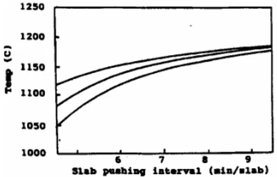
_out) multivariable process both for the regulatory and the supervisory control level. Therefore simplified low-order models were utilized for designing executive furnace controls of the regulatory level (see Eq. (4.3)). The regulatory design alone still remains confined to the framework of the first implementation of a human-operator supervised classical scheme of overall adjusted and locally fine tuned SISO controls. Subsequently, certain additional improvements have been made following appropriate engineering investigations. With the goal to exclude or reduce the role of human operator (except for the start-up/shut-dawn regimes), the research reported in here is along the same lines and an enhanced real-time process control ensuring about 4% cost saving for fuels has been achieved for furnace operations according to characteristics in Figures 1-2 [42].

Figure 3. Operating steady-state characteristics

desired: slab temperatures Tt, Tc, Tb as

functions of pusher pace; upper curve at slab top surface Tt, lower curve Tb - bottom surface,

and middle curve Tc – slab centre.

RZS furnace is primarily aimed at thermal treatment of low-grade steel slabs, before they enter the hot-rolling mill. When necessary, however, steel ingots are also processed for reasons of sustained run of the business, thus making its operation more delicate. Hence, the economic issue of energy saving is rather important.

Figure 4. Operating steady-state characteristics

desired: slab temperatures Tt, Tc, Tb as

functions of furnace heating zone temperature for the standard processing regime 1050-1250

o_{C (approximately achieved after the overall}

control system redesign)

Typical steel reheating takes place at the processing temperatures 900-1100 o_{C /}

1050-1250 o_{C / 1200-1400} o_{C, hence a process}

identification study was prerequisite in order to obtain families of steady-state (e.g., characteristics in Figure 4.2) and dynamic process models (e.g., pseudo-impulse responses and difference equations; see Figure 4.3) from the control point of view. The furnace is operated in a steady-state regime at a given pusher pace depending on slab/ingot size and other metallurgical specifications (beyond our expertise and not of concern in here) as shown by the respective characteristic curves in Figure 4.1 (the standard 1050-1250 o_{C processing).}

For the operating regime 1050-1250 o_{C, the}

respective characteristic curves of the heating furnace zones (lower and upper) for the slab temperatures are shown in Figure 4.2. It should be noted that the post-design observation showed that diagram may not be achieved entirely with full precision. In practice, it is likely that operating curves cannot be not that close to the linear ones, which has became apparent in the course of this design research study.

Finally, it is pointed out that any furnace control system design, when implemented, operates on the grounds of on on-line measurements of temperatures furnace walls, and not of slabs, for the constructive zones of the furnace. That is, in this case study, these are lower and upper heating zones and equalizing (or soaking) zone as shown in Figure 1. Characteristics curves for Tt and Tb

special measurement technology, whereas the one for Tc is estimated by some combined

empirical experimentation and analysis, or by a special Kalman filter, or by means of a special heat transfer simulation model.

The main goal of the overall control system is to ensure such a characteristic curve Tc for the

inside temperatures of the slab, which guarantees its quality mechanical processing in the associated hot-rolling mill. Further, it should be noted that slabs are heated mainly due to radiation transfer from hot furnace walls, and convection heat transfer due to forced counter-flow of hot gases is minor (see Figure 1) Besides, slabs are sliding on the tracks when pushed and, turn, these cause slightly lower heated skid-marks at the bottom side of slabs. Fore these reasons, it is important to achieve heating zone operating characteristics close to the ones in Figure 4.2 albeit not entirely linear.

4.1. Process Identification Study and Regulatory Control Level Design

Pragmatically, with such a real-world furnace and within given plant environment and operating conditions, the re-design study for further control based improvements started with identification of a family of steady-state (SS), convex non-linear, input/output equations (static I/O control characteristics) representing “energy

supply

m

_j/ controlled temperatures

T

_i” in

terms of slab temperatures at furnace walls (which predetermine temperatures top and bottom slab surfaces), and the pseudo-impulse response (weighting) sequences by using admissible control inputs (with regard to allowable magnitude ranges) around the three typical operating points of low (30%), medium (60%), and normal or maximum loads (higher than 80%). That is, the static I/O characteristics and the pseudo-impulse I/O weighting patterns as follows: i k j i i

f

m

m

const

k

j

y

T

=

(

;

=

,

≠

)

=

, out

N

i

=

1

,

, (4.1) at steady-state operation

t

_SS

=

{ }

t

_{SS OpPoint}, and

[

(

)

]

[

(

)

]

,

inp out N N ij

t

g

t

G

=

_×

t

₀

≤

t

≤

t

_SS

<

t

_∞. (4.2)

These were identified under operating conditions. Note, these are readily made discrete with respect to the time through the identification signal processing.

Figure 5. A sample case of step-response tests

at the steady-state operating temperature 1150

o_{C; measurement gradation of time in [min]}

and of temperature in tens of [o_C]

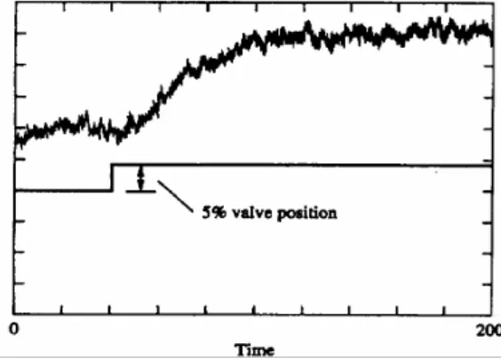
In principle, any method for identification and signal processing may be used for such dynamical processes [43]. However, for the furnace under operating conditions [18] the input signals had be confined in ranges from (0.03-0.05) to (0.10-0.15) of the maximum magnitude of executive control inputs. Following a choice of 5-10% of the maximum input signal (fuel flow) allowed (% valve opening in Figure 4.3) and the records of a number of step responses for every input, respectively, it was feasible to obtain the families of chosen models pointed out below.

There have resulted families of traditional time-first-order-lag (Ziegler-Nichols) and dead-time-second-order lag (Küpfmüller-Strejc) with ranges of values according to typical operating loads [16], [17] as well as of non-parametric dynamical models in terms of k-time sequence matrices of the respective process weighting matrix function. Process dynamics is a typical one (see Figure 4) and non-periodic, which may be approximated by a ‘pure’ time-delay and ‘inertial’ time-lag. Combining these results with model PRBS-response identification (see Figure 5) and relevant data processing (MATLAB-Systems Identification Toolbox) it was possible to obtain sets of fairly good time-delay first and second order models such as

)

1

)(

1

/(

)

exp(

)

(

s

=

K

−

s

T

₁

+

T

₂

s

+

G

_{ij ij}

τ

_ij , (4.3) here matrix of process gains is given by

K

=

Q

∆

∆Θ /

. Thereafter the respective discrete-time representations in shift-operator

q

−1 are derived.

Figure 6. PRBS response of controlled

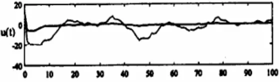
temperature for reheating channels ‘upper zone’ and ‘lower zone’ (PRBS signal optimum design T = 31 and ∆t = 1 [min] by Stankovski and co-authors, 1999)

Besides, on the grounds of a series of step-response identification it was possible to identify value ranges for the main attributes of slab heating process dynamics: steady-state (SS) gains

K

_ij (in [o_{C/MJ/min]) and pure time-delays}

(dead-times)

τ

_ij (in [min]) within each of the

process transfer paths. Regarding main process channels (transducer-actuator paths of the equalizing, lower, and upper zones) the values of SS gains range within 7.25-8. 95, 4.10-6.50, and 1.50-1.70, while time-delays within 1.50-1.70, 2.10-3.90, and 3.90-7.20, respectively, depending on the actual power load (see Figures 4 and 5); these variations account for operating process uncertainties to some extent.

Static I/O control characteristics appeared not to be symmetric entirely (Figure 6) and showed that, should the furnace process is regarded as a multi-input-multi-output one, dynamical weighting sequences were not entirely symmetric either with regard to the main process channels (Figure 7). For these reasons, it was decided and carried out a re-design study on

transducer-actuator collocation resulting in a certain correction of the initial distribution locations.

Figure 7. Estimates of operational variations

in time delays for the three furnace zones as seen via step responses, caused by load variations and other disturbances; the middle one for the equalizing and side ones for the upper and lower zones, respectively

For pragmatic reasons, thermal processes in industrial furnaces, having finite steady states, stimulate the use of the well-known methods of statistic regression analysis (for the input-output control characteristics) and of step-response and maximum-length PRBS-response (for the process dynamics); three families of dynamic models according to the main operating power loads. After appropriate filtering, all these models are easily mapped into time sequences truncated at time

N

_t and then k-time sequence matrices

[

g

_ij

(k

)

]

,

t

₀

=

k

₀

≤

k

≤

k

_Nt , obtained with an appropriate sampling period

T

_s (Ts = 1

min for RZS furnace); that is, a Toeplitz operator is derived from the sequence of MxM (

N

_inp

×

N

_out) Markov matrices

G

(k

)

of plant pseudo-impulse responses [7]. These models may be turned into matrices of approximate channel-transfer functions in shift operator

q

−1. Equivalent discrete-time state-equation realisations via dyadic forms are readily derived thereafter. In turn, identified models in all forms relevant to the time domain were made available:

[

(

)

]

*

(

)

)

(

k

g

l

m

k

y

t inp out N N N ij

G

G

× ×

=

, t N

k

k

l

k

t

₀

=

₀

≤

≤

≤

, (4.4) with

[

]

t inp out N N N ij

l

g

(

)

_{× ×}

≅

[

]

∞ × ×N N N ij inp out

l

g

(

)

if and only if t N N

lim

→

{

[

]

}

N N N ij

l

_{out inp}

g

0

)

(

_× =

= ) 1 (

lim

+ → Nt N

{

[

]

}

N N N ij inp out

l

g

0

)

(

_× ;

[

(

)

]

(

)

)

(

1 1 1 d N N

m

q

q

G

q

y

inp out − − × − −

₌

G

G

; (4.5)

[

(

)

]

(

)

[

(

)

]

(

)

)

1

(

k

A

T

x

k

B

T

m

k

d

x

inp N n s n n s

+

−

=

+

_×

G

_×

G

G

[ ]

(

1

)

)

1

(

k

+

=

C

_×

x

k

+

y

_{Nout n}

G

G

. (4.6) Hence, all the information needed for writing down suitable identified models of the class (3.1) for the three main process channels was gathered.

It should be noted, there exist methods and techniques in the literature, in particular see Ljung (1999) for direct identification of models of the class (3.1) needed. However, we believe that the way we conducted our modeling and identification study is more appropriate in solving real-world systems engineering design problems because it enables gathering a deeper insight into the operating features of the given plant in the given filed environment, and under typical working regimes it is operated. In turn, a thorough physical understanding is gained on the entire control systems infrastructure, which is designed to be implemented on a real-world plant such as a high power (28/25 MW) industrial furnace. Thus it can be argued that, with such a deeper insight into both steady states and transients controlled by the regulatory level at hand, one shall have a deeper understanding on the governing function the supervisory control level is supposed to perform.

Figure 8. Theoretical closed-loop step

performance of a SS-decoupling plus PI regulatory control level

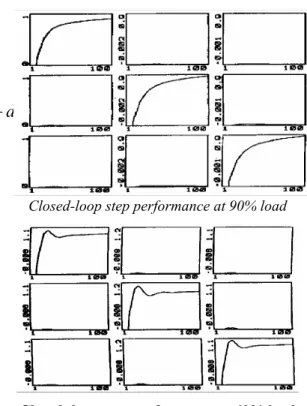
Closed-loop step performance at 90% load

Closed -loop step performance at 60% load

Closed -loop step performance at 30% load Figure 9. Closed-loop control performance of

the regulatory level alone; the same design of simple SS-decoupling plus PI regulatory controls operated at different loads (the noise is filtered out).

The control design of the regulatory level is discussed with few details. It is pointed out that the simple steady-state (SS) decoupling plus traditional decentralized PI control laws are employed, where the local proportional actions are made compliant with the proportional SS decoupling gains. These deigns were made to ensure the closed-loop stability and a fairly good transient performance with no SS offsets, of course. Theoretically, closed-loop performance for unit-step reference commands would be as depicted in Figure 8; however, practically some

time delay in controlled temperature responses remains as seen in Figure 9. Note, SS decoupling gains are determined by the way in the course of the above described identification analysis and experimentation.

A family set of such regulatory control designs have been determined, given the availability of families of models for operating regimes at different loads. (This supports further the precedent argument of ours above.) What matters is that the resulting regulatory level design for operating load about 90% of the furnace capacity alone is capable to achieve the performances illustrated by means of the closed-loop step-responses in Figure 4.7. Consequently, the proper performance of the regulatory level has been met, which in turn was a prerequisite in order a good feasible design of the supervisory level to be carried out.

4.2 Further Identification Modeling and Supervisory Level Design

In the sequel the design of the supervisory control level is discussed. For the supervisory level, clearly, as long as the correct representational relationship between pure delay and inertial times are captured into the discrete-time models of the main process channels (equalizing, lower, and upper zones). For the sake of reducing the computational effort, time-delay-first-order models were adopted in stead of equation (4.3).

On the grounds of the identification study, physical parameter values (pure delays, time constants, process gains) were chosen within the ranges for the normal operating, high power load and initial conditions within processing temperatures 1050-1250 o_{C. That is,}

ii

τ

=3.90-7.20,

K

_ii=1.50-1.70,

y

_i

(

0

)

=1150 o_{C. The}

latter, in turn, implies non-zero initial values for executive control variables

u

_i

(

0

)

=

U

_midrange representing the mid-range control values on the top of which controls

u

_iit

=

δ

u

_ii

(t

)

)

(

t

j

u

u

t j _ii

ii

=

+

+

_δ

_{, due to the supervisory}

controller, are added. The process noise vector

)

(

t

e

was assumed to have the same stochastic characteristics in every channel and

approximated as a weak white noise with

2

e

σ

=10.

The residing horizon for the supervisory predictive control can be determined by observing the pure time delays and the relationship between pure delay and inertial times

δ

=

τ

_ij

/(

τ

_ij

+

T

_ij

)

and

η

=

τ

_ij

/

T

_ij [16] taking into consideration the adopted sampling period

T

_s

=

1

[min]; that is, by observing the integer value of

d

=

[

τ

_ij

T

_s

]

. Since

τ

_ij is approximately the same for the main channels of the upper and lower zones (i.e.,

ii

=

1 and

3

) and not equal to the one of the equalizing zone (i.e.,

ii

=

1 and

3

) as seen from Figure 4.5, a common average time delay

τ

_av was adopted and used throughout. In turn, it appeared that the residing horizon should have minimum

H

_r

=

3

and maximum

H

_r

=

5

sampling periods; the former can further reduce the computational effort, but the latter can contribute to the quality of supervisory control design.

The resulting controlled autoregressive and moving-average model [4], with regard to

[

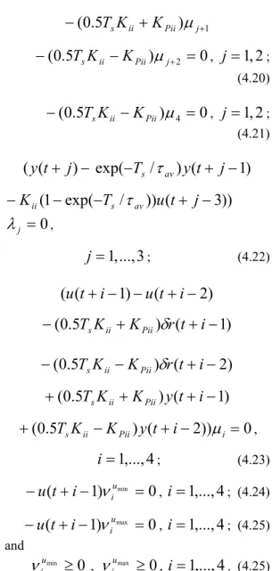
ii

T

s

]

d

=

τ

, have the form:

∆

+

=

− −

₎

₍

₎

₍

₎

₍

₎

₍

₎

_/

(

_q

1

_y

_t

_B

_q

1

_u

_t

_e

_t

A

_{ii i ii i ij} (4.7) with 1 1

₎

₁

_exp(

_/

₎

(

q

−

=

−

−

T

q

−

A

_{ii s}

τ

_av , ) 1 ( 1

₎

₍

₁

_exp(

_/

₎₎

(

d av s ii ii

q

K

T

q

B

−

₌

₋

₋

_τ

− + _.

Since the regulatory level consists of PI controllers “

K

_Pii

+

K

_Iii

/

s

” (which are acting

on error signals “

r

_ii

(

s

)

−

y

_ii

(

s

)

≡

r

_i

(

s

)

−

y

_i

(

s

)

” with

K

_Pii

and

K

_Iii designs to produce controls “

u

_ii

(

s

)

≡

u

_i

(

s

)

”; elaborated in the regulatory control level) Eqs. (3.1) become:

)

(

)

(

)

(

)

(

)

(

)

(

_q

1

_u

_t

_B

_q

1

_r

_t

_B

_q

1

_y

_t

A

i ry i i rc i i rc − − −

₌

₊

(4.8) with 1 1

₎

₁

(

q

−

=

+

q

−

A

i rc ,