A SURVEY OF VALUE AT RISK METHODOLOGIES
EL F YET M 105624003
STANBUL B LG ÜN VERS TES SOSYAL B L MLER ENST TÜSÜ
F NANSAL EKONOM YÜKSEK L SANS PROGRAMI
EGE YAZGAN
A SURVEY OF VALUE AT RISK METHODOLOGIES
RISKE MARUZ DE ER YÖNTEMLER YLE LG L B R NCELEME
EL F YET M 105624003
Ege Yazgan :………
Koray Akay :………
Orhan Erdem :………
Tezin Onayland121 Tarih :
Toplam Sayfa Say1s1 : 43
Key Words Anahtar Kelimeler 1) Parametric value at risk 1) Parametrik riske maruz de2er
2) Historical value at risk 2) Tarihsel riske maruz de2er 3) Weighted Historical value at risk 3) A21rl1kland1r1lm1= tarihsel riske maruz de2er 4) Monte Carlo value at risk 4) Monte Carlo riske maruz de2er 5) Filtered Historical value at risk 5) Süzülmü= tarihsel riske maruz de2er
ABSTRACT
In Section 1, it is given an introduction. In section 2, it is provided Parametric VaR Methodology based on explicit assumptions for factor returns that pricing functions are linear in the risk factor returns. Section 3 and section 4 describe two different methodologies to asses these risk. The first methodology is based on Monte Carlo simulation and does not make any analytical assumption regarding the pricing function of the underlying positions. The second methodlogy is HS which based on historical fequencies of returns. Section 5 and section 6 explains two different methods to examine risk based on these historical frequencies of retuns. In section 5, WHS which assignes higher weight to new observations and a lower weight to older observations. In section 6, FHS is introduced. It is shown how it eliminates the problem with irrelevant current regime by scaling historical observations by an estimate of their volatility. Finally, it is concluded in section 8.
ÖZET
Birinci bölüm giri= k1sm1d1r. kinci bölümde parametrik riske maruz de2er yöntemi, fiyat fonksiyonlar1yla risk faktöru getirileri aras1nda linear bir ili=ki vard1r varsay1mi alt1nda incelenmektedir. Üçüncü ve dördüncü bölümlerde bu riski incelemek için iki farkl1 yöntem daha sunulmaktad1r. Birincisi Monte Carlo simulasyon yöntemidir. Bu yöntem fiyat fonksiyonlar1 ve risk faktör getirisi aras1ndaki ili=kiyle ilgili her hangi bir analitik varsay1mda bulunmaz. kincisi tarihsel simulasyon yöntemidir. Bu yöntem geçmi= risk faktörü verilerinin getirilerini kullanarak risk incelemesi yapar. Be=inci bölümde, a21rl1kland1r1lm1= tarihsel simulasyon yöntemi incelenmektedir. Bu yöntem, riski geçmi= verilere bugünden geçmi=e azalarak a21rl1kland1rma vererek incelemektedir. Alt1nc1 bölümde, süzülmü= tarihsel simulayon yöntemi incelemektedir. Bu yöntem geçmi= risk faktör getirilerini ölçeklendirerek =imdiki rejimle iligili olu=abilecek problemi yok etmeye çal1=1r. Yedinci bölümde sonuç k1sm1n1 veriyorum.
TABLE OF CONTENTS
1 INTRODUCTION...1
2 PARAMETRIC VaR METHODOLOGY...5
2.1 ParametricVaR with one source of risk...5
i. Historical average...7
ii. Exponentially Weighted Moving Average...7
iii. Generalized Autoregressive Conditional Hetereoscedastic ...8
2.2 Applying Parametric VaR methodology ...9
2.3 Parametric VaR with multiple sources of risk...9
2.4 Advantages & Disadvantages...10
3 HISTORICAL SIMULATION VaR METHODOLOGY ...11
3.1 Historical Simulation VaR...11
3.2 Applying Historical Simulation VaR methodology ...11
3.3 Historical Simulation VaR with multiple sources of risk...13
3.5 Advantages & Disadvantages...15
4 MONTE CARLO SIMULATION VaR METHODOLOGY ...16
4.1 Monte Carlo Simulation VaR ...16
i. Simulating Markov process...16
ii. Geometric Brownian Motion ...19
iii. Simulating yields...22
4.2 Applying Monte Carlo Simulation VaR Methodology ...24
4.3 Monte Carlo Simulation VaR with Multiple Sources of Risk...25
5 WEIGHTED HISTORICAL SIMULATION VaR METHODOLOGY ...30
5.1 Weighted Historical Simulation VaR with One Source of Risk ...31
5.2 Applying Weighted Histrical Simulation ...32
5.3 Weighted Historical Simulation VaR with multiple sources of risk ...35
5.4 Advantages & Disadvantages...36
6 FILTERED HISTORICAL SIMULATION VaR METHODOLOGY ...37
6.1 Filtered Historical Simualtion VaR ...37
6.2 Applying Filtered Historical Simulation ...38
6.3 Filtered Historical Simulation VaR with multiple sources of risk ...39
6.4 Advantages & Disadvantages...41
7 CONCLUSION ...43 REFERENCES
LIST OF TABLES
Table Page
3.1 HS -VaR calculation steps with one source of risk 12
3.2 HS-Portfolio P&L with multiple source of risk 14
5.1 WHS -VaR calculation steps with one source of risk 35
5.2 WHS-Portfolio P&L with multiple source of risk 36
6.1 FHS -VaR calculation steps with one source of risk 40
6.2 FHS-Portfolio P&L with multiple source of risk 42
LIST OF FIGURES Figure
1.1 VaR revolution 3
4.1 Wiener process 18
4.2 Simulating price path 22
4.3 Simulating price paths 23
4.4 Simulating interest rate path 25
1 INTRODUCTION
Value-at-Risk1(VaR) was generally used for measuring market risk2in trading portfolios as a risk measurement at the begining of 1990s (http//www.riskglossary.com/link/value at risk, para. 7 and Jorion, 2001, p.22). Its roots can be traced back as far as 1922 to capital requirements the New York Exchange. Also, VaR has origins in portfolio theory3 and crude VaR measure published in 1945 (Holton, 2002, p.1). Till Guildmann can be seen as the inventor of the name value at risk while head of global reserch at J.P. Morgan in the late 1980s (Jorion, 2001, p.22).
VaR was firstly used by major financial firms in the late 1980’s to measure the risks of their trading portfolios. Currently VaR is used by large financial firms. Also, it is increasingly being used by smaller financial institutions, non-financial corporations, and institutional investors (Linsmeier and Pearson, 1996, p.2).
During 1990s number of organizations4 -including Orange Country, Barings Bank, Metallgesellschaft, Daiwa Bank and Sumitomo Corporation- suffered staggering losses due to speculative trading, failed hedging programs or derivatives. In Particular, in adequacy of traditional measures of exposures and the move toward mark-to-market both cash instruments and derivatives represented a new challenge for risk measure. And VaR has been revealed as a risk measure from the recognition that a tool which is needed accounts for various sources of risk and expresses loss in terms of probability. Until then, risk was measured and managed at the level of a desk or business unit (Holton, 2003, p.21).
The concept of the VaR approach depends on Harry Markowitz portfolio selection paper. Markowitz (1952) firstly used the volatility of return as a risk metric by emphasising on the tradeoff between expected return and volatility in a period as a risk measure5 (http//www.riskglossary.com/link/value at risk, para 8). Roy (1952) firstly mentioned a
confidence-based risk measure. He defended selecting portfolios that minimize the
1See Holton (2003) for the history of VaR and seeLinsmeier and Pearson (1996) and Jorion (2001) for a
general introduction to VaR. Also, see Duffie and Pan (1997) for the overview of various approaches to calculate VaR.
2For more inforemation on the market risk disclosure rules, see www.bis.org. The actual text is at http://www.bis.org/publ/bcbs119.pdf.
3See Jorion (2001), pp: 147-153. 4See Jorion (2001), pp: 34-43.
possibility of a loss greater than a catastrophic level. In addition, Baumol (1963) advocated a risk mesurement depends on a lower confidence limit at some confidence level (Jorion, 2001, p.115).
In the following years, many risk metrics has been used to manage risk exposures of the uncetainity. Because VaR metric gives institutions the ability to find out any mis-hedges portfolios before a loss incurred by describing probabilistically the risk of these portfolios, it is accepted as a risk metric in finance. It describes some of the basic issues involved in measuring the market risk of a financial firms’ book, the list of positions in various instruments that expose the firm to financial risk ( http://www.riskglossary.com/link/value
at risk, para.2).
VaR measures the worst expected loss under normal market conditions over a specific time interval at a given confidence level. As one of my reference states: “ VaR answers the question: How much can be lost with x % probability over a pre-set horizon” (J.P Morgan, RiskMetrics-Technical Document). Another way of expressing this is that VaR is the lowest quantile of the potential losses that can occur within a given portfolio during a specified time period (Longerstaey, 1996, p.6).
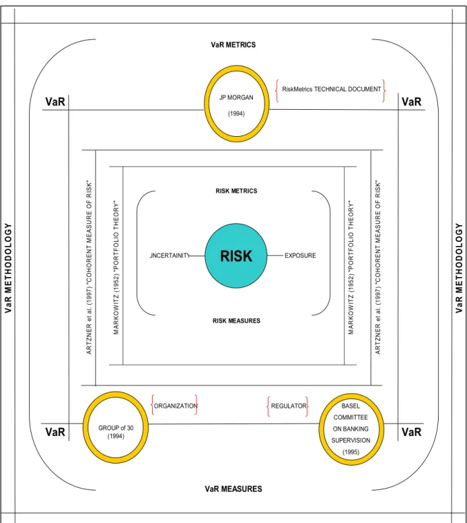
The calculation of VaR is straightforward, but its implementation is not. (Marshall and Siegel, 1996, p.3, Benninga and Wiener, 1998, p.2). The concept of VaR is not new. So that, the methodology behind VaR is not new. It results from merging of financial theory, which focuses on the pricing and sensitivity of financial instruments, and statistics, which studies the behaviour of the risk factors (Jorion, 2001, p.257). The VaR revolution6started in 1993. It has originated the Group of 30 (1993), JP Morgan RiskMetrics system (1994) and the Basel Committee on Banking Supervision (1995).
VaR has many applications such as in risk management to evaluate the performance of risk takers because regulators require financial institutions backtest their internal VaR methodologies7. In particular, the Basel Committee on Banking Supervision (1996) at the bank for international Settlements dictates to financial institutions such as banks and
6See Jorion (2001), pp: 43-49.
7See Lopez’ s paper (1996) paper answers the question of how regulators should evaluate the accuracy of
investment firms to meet capital requirements based on VaR estimates. So that, it is very important to develope methodologies that provide accurate estimates.
Figure 1: VaR revolution
In this context, there are three traditional VaR methodologies. Firstly, Parametric Methodology is based on the parametric distribution assumption for risk factor returns to calculate VaR. Secondly, Historical Simulation is based on empirical distribution assumption of actual historical data to calculate VaR. Thirdly, Monte Carlo Simulation is based on pesudo random generated factor returns’ distribution to calculate VaR. Thus, VaR calculation requires the calculation a quantile of the distribution of returns.
ORGANIZATION REGULATOR
RiskMetrics TECHNICAL DOCUMENT
VaR VaR VaR VaR VaR METRICS RISK MEASURES JP MORGAN (1994) GROUP of 30 (1994) BASEL COMMITTEE ON BANKING SUPERVISION (1995) VaR MEASURES V a R M E T H O D O L O G Y V a R M E T H O D O L O G Y M A R K O W IT Z (1 95 2 ) "P O R T F O L IO T H E O R Y " M A R K O W IT Z (1 95 2 ) "P O R T F O L IO T H E O R Y " A R T Z N E R e t a l. (1 9 97 ) "C O H O R E N T M E A S U R E O F R IS K " A R T Z N E R e t a l. (1 9 97 ) "C O H O R E N T M E A S U R E O F R IS K " EXPOSURE UNCERTAINITY RISK METRICS
RISK
The main objective of this paper is to survey of VaR methodologies8 by comparing on weakness and strength of each one. It is wanted to focus on the logical flaws of the methodologies and not on their empirical application. In order to facilititate comparison, it is restricted the attention to four methodologies. The paper is organized as follows: In section 2-6, it will be given a survey of Parametric VaR, Historical simulation VaR, Weighted Historical simualtion VaR, Monte Carlo simulation VaR and Filtered Historical simulation methodologies in theoretical foundations. In Section 7, it will be concluded.
8It is refered the interested reader to the excellent web sites www.gloriamundi.org,www.riskglossaryand www.ssrn.org,www.riskcenter.com for a comprehensive listing of VaR contributioms.
2 PARAMETRIC VaR METHODOLOGY
This chapter introduces Parametric VaR Methodology. Section 2.1 works in a simple case with just one source of risk. Section 2.2 shows how to apply this methodology to construct VaR calculation. Then multiple sources of risk are considered in Section 2.3. Finally, advantages and disadvantages of the methodology are introduced in Secion 2.4.
2.1 ParametricVaR with one source of risk
This section introduces Parametric VaR Methodology with one source of risk. The idea behind VaR calculation with this methodology is “to approximate the pricing functions of each standardized position in order to obtain a formula for VaR and other risk statistics” (Mina and Xiao ,2001, p.21). This methodology works under the assumption that the P&L of a portfolio are linear in the underlying risk factors. It can be expressed as a linear combination of risk factor returns9 by using a first order Taylor series expansion. The construction of this methodology relies on two assumptions: Linearity and normality assumptions.
• Linearity assumption:
Let us assume that there is a single position dependent on n risk factors denoted by P
( )
rf i ,n i=1,..., .
1. The present value PV of the position is approximated by using a first order Taylor series expansion in order to construct Parametric VaR Methodology to be able calculate VaR.
( )
( )
( )
( ) ( )
1 n PV PV P rf P rf PV P rfi P rfi P rf i i + + = 2.19Note that Taylor series expansion uses actually percentage returns
( )
( )
P rf i r
P rf i
= , but this model relies on the logarithmic returns normality assumption. So that, an additional assumption is made to be consistent with this distributional assumption that is 1 1
0 0
log P P 1
P P . For further description , please see (Mina and
( )
(
)
( )
( ) ( )
1 n PV PV P rf P PV rfi P rfi P rf i i + = 2.2( ) ( )
& 1 n PV P L P rf i P rf i= i 2.3( )
( ) ( )
( )
& 1 n PV P rfi P L P rf i P rf P rf i= i i 2.4In other words, the equation 2.3 says that when the underlying risk factor changes, then the profit and loss of the position approximately changes by the sensitivity of the position to changes in that linear risk factors (Mina and Xiao, 2001, p.21).
2. Now, the change in present value can be approximated as
( ) ( )
& 1 n P L i r i i= 2.5 1 2 1 2 & ... n n P L r + r + + r 2.6 ' & P L= r 2.7 where( )
( )
( ) ( )
P rfi i P rfi P rfi= and it is called the delta equivalents for the position. They can be interpreted as “the set sensitivities of the present value of the position with respect to changes in each of the risk factors” (Mina and Xiao, 2001, p.21).
• Normality assumption:
An other assumption to construct VaR calculation with this methodology is normality assumption of risk factor returns. Since each risk factor return is normally distributed, the P&L distribution under the parametric assumptions is also normally distributed with mean zero and variance P& ~L N
(
0, ')
. Then, VaR is calculated as a percentile of this P&L distribution. That percentile of the normal distribution is multiple of the standard deviation of a portfolio (Mina and Xiao, 2001, p.23). In other words,P,t+1
=
'
t t+1 tThus, it is obtained a formula for VaR and other risk statistics by approximating the pricing functions of each standardized position. The VaR calculation requires only a volatility estimation10 of the portfolio’s change. Return RiskMetrics: The Evaluation of a Standard11 (2001) chaper 2, Jorion’s Financial Risk Manager handbook12 (2003) chapter 17, Jorion’s Value at Risk13 (2001), Dowd’s Beyond Value at Risk14 (1998) and Hull15 (1997) chapter 16 are useful resources to understand the theory of parametric VaR Methodology. Three different models are generally used to estimate volatility16: Historical Average (HA), Exponentially Weighted Moving Average (EWMA) and Generalized Autoregressive Conditional Heteroscedastic (GARCH) model. Let us briefly examine these models.
i. Historical average
If it is assumed that conditional expectation of the volatility is constant and the daily return has zero mean, the proper estimate of the volatility;
n 2 i i=1
1
s=
r
n -1
2.9where is the estimated volatility, n is is the sample size and r is the daily return.
The weakness of this model is of course constant volatility assumption. This estimate of the volatility could not mimic the big changes in the volatility and remains nearly constant where the sample size increases.
ii. Exponentially Weighted Moving Average
EWMA past observations with exponentially decreasing weights to estimate volatility. Therefore, this is a modified version of historical averaging. Instead of equally weighting, in EWMA weights differ. The estimated volatility can be shown as;
10 Christofersen, P., 2003, Elements of Financial Risk Management, Academic Press.
11
Mina, J., and Xiao, Y. X., 2001,Return to RiskMetrics: The Evaluation of a Standad, RiskMetrics Group.
12Jorion, P., 2001, Value at Risk: The New Benchmark for Managing Fianacial Risk, McGraw-Hill, Second
Edition.
13 Jorion, P., 2003, Financial Risk Manager Handbook, Wiley Finance, Second Edition
14
Dowd, K., 1998, Beyond Value at Risk: The New Science of Risk Management, John Wiley & Sons, England.
15 Hull, John C., 1997, Options Futures, and Other Derivatives, Prentice-Hall, Third Edition
16 Christofferson and Diebold (2000) investigate the usefulness of dynamic variance models for risk
(
)
2 2 2 1 1 t t = r + t 2.10 2 t=
t 2.11By repeated substitutions it can rewritten the forecast as;
(
)
2 1 2 11
n i t t i=r
=
2.12Equation 2.11 show the volatility is equal to a weighting average. The weights decrease geometrically. The value of decay factor estimated simply by minimizing the one week forecast errors.
iii. Generalized Autoregressive Conditional Hetereoscedastic
The family of ARCH17 models was introduced by Engle (1982) and Bollerslev (1986). The Generalized ARCH model of Bollerslev (1986) defined GARCH by;
t t t
r
= +
µ
2.13(
)
2 2 2 1 1 q p t i t i j t j i=r
µ
j== +
+
2.14 2 t t = 2.15GARCH imposes that the proper volatility estimate is based on nots only the recent volatilities but also previous forecasts which include the previous volatilities. Then the GARCH model is a long memory model. The parameters of the GARCH can be estimated by a Maximum Likelihood procedure.
2.2 Applying Parametric VaR methodology
It has already been mentioned the content of the Parametric VaR Methodology. Now is the time to make up for the steps of calculation VaR. Linsmeier and Pearson18 (1996) explain computation of VaR for one source of risk using Parametric VaR Methodology in four steps:
1. Risk Mapping: The first step is to map the position by determining the underlying risk factors and the standardized positions which are directly related to the risk factors.
2. Statistical Analysis for Risk Factors: The second step is to estimate the parameter of risk factor returns depending on the underlying linearity and normality assumptions..
3. Statistical Analysis for Standardized Positions: The next step is to identify the volatilities and correlations of changes in the value of the standardized positions. 4. Portfolio Variance-Covariance Procedure: This step is the key, which includes
identifying volatility of changes in mark-to-market portfolio value.
The process explained above applies to a single risk factor. As it will be illustrated, the model can be generalized to describe the dynamics of multiple risk factors.
2.3 Parametric VaR with multiple sources of risk
It is now turned to the more general case of the methodology with many sources of financial risk. This section introduces Parametric VaR Methodology with multiple sources of risk which requires an additional work.
Let us assume that there is m positions denoted by
P L
&
j, j=1,...,m. Due to deltaequivalents aggreagtion properties, after calculating independently delta equivalent for each position, they are aggreagted to obtain the delta equivalent for the position( Mina and Xiao, 2001, p.23). In other words,
18 Linsmeier, T. And Pearson, N.,1996, Risk Measurement: An Introduction to Value at Risk, University of
( )
= = = m j m j T portfolior j L P L P 1 1 & & 2.16 r L P m j T portfolio =1 & 2.17The general finding of this methodology is that it imposes strong assumptions about the underlying risk factors as it has been mentioned in section 2.1. The empirical evidence about the distributional properties of risk factor changes provides evidence against these assumptions, e.g. Kendall (1953), Mandelbrot (1963) and Fama (1965).
It has already been mentioned the process of calculating VaR by using the parametric VaR methodology, but so far the content has not been precise regarding its pros and cons. Now is the time to make up for that.
2.4 Advantages & Disadvantages
Jorion19 (2001) explains the pros and cons of this methodology as the following:
Advatages
• The main benefit of this approach is its simplicity.
Disadvantages
• Unlike HS VaR Methodology and WHS VaR Methodology, it requires parametric estimations such as volatilities, correlations or other parameters and thus does not maintain the ease of implementation .
• Unlike MCS VaR Methodology, it cannot account for nonlinearity effects.
• It may also underestimate the occurance of large observations beacuse of its reliance on a normal distribution.
19Jorion, P., 2001, Value at Risk: The New Benchmark for Managing Fianacial Risk, McGraw-Hill, Second
3 HISTORICAL SIMULATION VaR METHODOLOGY20
Recognizing the fact that most underlying risk factor returns cannot be described by a theoretical distribution, an increasing number of financial institutions are using historical simulation.
This chapter introduces Historical Simulation VaR Methodology . Section 3.1 works in a simple case with just one source of risk. Section 3.2 shows how to apply this method to construct VaR calculation. Then multiple sources of risk are considered in Section 3.3. Finally, advantages and disadvantages of the methodology are introduced in Section 3.4.
3.1 Historical Simulation VaR
This section introduces Historical Simulation VaR Methodology with one source of risk. It is “a simple, atherotical methodology that requires relatively few assumptions about the statistical distributions of the underlying risk factor returns to obtain future portfolio’s profits and losses (P&L) distribution” (Linsmeier and Pearson, 1996, p.2). The basic main assumption behind historical simulation is that changes in the undelying risk factors are identical to the looked at changes in those over a sample period (Mina and Xiao, 2000, p.26). That is, the historical data speak fully about the distribution of future return without dictating any further assumptions (Christofferson, 2003, p.101). This means that a historical simulation is performed by sampling from past returns, and applying them to the current level of the risk factors to obtain risk factor price scenarios. And then, these price scenarios are used to obtain P&L scenarios for the portfolio.
It has been already mentioned the content of the HS approach. Now is the time to make up for the steps of calculation VaR.
3.2 Applying Historical Simulation VaR methodology
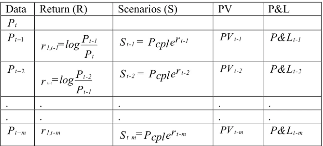
Linsmeier and Pearson (1996) explains the computation of VaR for a portfolio using historical simulation VaR methodology as the following steps:
1. Risk mapping: The first step is to identify n risk factors rfi, with i=1,...,n . 2. Data: The next step is to collect historical values of n risk factors for the last
determined period.
3. Return: This step includes obtaining risk factor returns.
4. Secanarios for risk factor price levels: This is the key step which attempts to obtain a
formula expressing the mark-to-market value of the position in terms of each risk factor subjecting to current price level Pcpl.
cpl k S P ,trf i log = e Prfi, P P ,t-1 rf i 3.1
where i=1,...,n. That is, if there is an instrument in a position and it contains n risk factors , the scenarios (S) of each future are obtained by expressing prices in a function of logarithmic returns of each risk factor. The current portfolio is subjected to the percentage changes in risk factors and prices experienced on each of determined period.
5. PV of instrument: This step expresses the present value of an instrument as a fuction
of the n risk factors rfiwith i =1,...n.
6. Portfolio P&L: The profits and losses of a portfolio are calculated.
7. Sorting portfolio P&L: The next step is to order the mark-to-market profits and losses
from the largest profit to the largest loss.
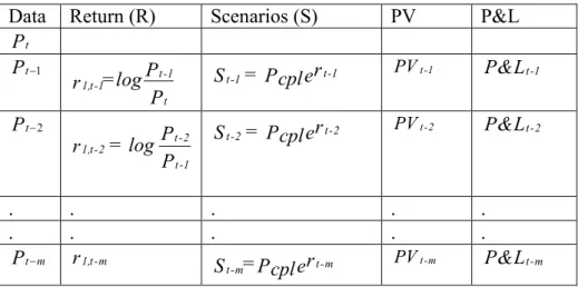
Table 3.1 HS-VaR calculation steps with one source of risk
Data Return (R) Scenarios (S) PV P&L
t P 1 t P t-1 1,t-1 t P =log r P t-1 t-1= r S Pcple PVt-1 P&Lt-1 2 t P 1,t -2 t-2 t-1 P =log r P t-2 t-2= r S Pcple PVt-2 P&Lt-2 . . . . . . . . . . t m P r1,t-m St-m=Pcplert-m PVt-m P&Lt-m
Finally, the loss which is equaled or exceeded p percent of the time is selected. Using the probability of p percent, this is the value at risk. That is,
(
)
{
}
{
}
(
)
, log 1 ,1 , 1 , 1 1 ,1 & 1 1 1 & ,1 1 m Prf i t percentile NV p VaRp t Pcpl e P t rf i i m percentile P Li i p m percentile P LT m i p m i = "" × # # + $ % = $ % = = = "" & # # $ % = $ %(
)
1 1 & ( ) p F P L k = =where k =
(
1 p)
m. As the VaR typically falls in between two observations, linear interpolation can be used to calculate exact number. Thus, VaR is simply the lower percentile of the portfolio P&L distribution.The process explained above applies to a single risk factor. As it will be illustrated, the model can be generalized to describe the dynamics of multiple risk factors.
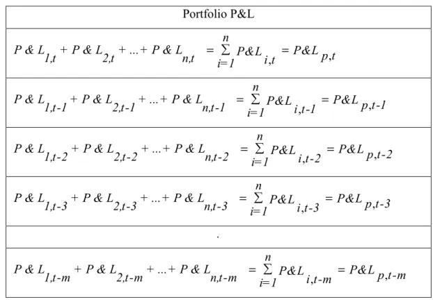
3.3 Historical Simulation VaR with multiple sources of risk
It is now turned to the more general case of simulations with many sources of financial risk. This section introduces Historical Simulation VaR Methodology with multiple sources of risk which requires an additional work.
Let us assume that there is m positions denoted by
P L
&
j, j=1,...,m. After summing profitsand losses for each position for each day, they are ordered from the highest profit to lowest loss.
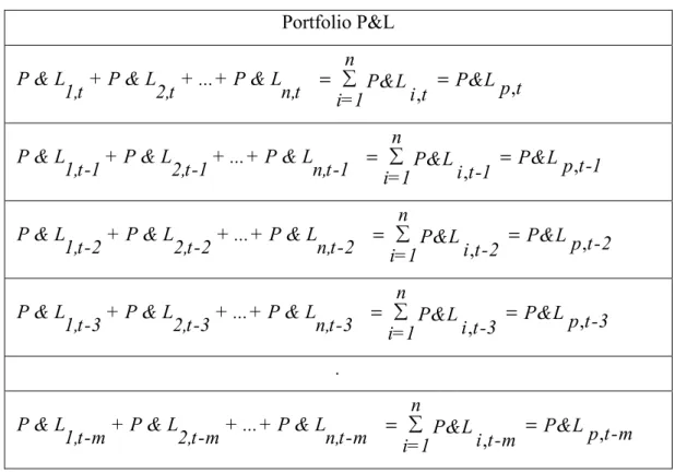
Table 3.2 HS-Portfolio P&L with multiple source of risk Portfolio P&L
, ,
n
P & L1,t + P & L2,t + ...+ P & L n,t P&L P&Lp t i t i=1 = = , , n
P & L1,t-1+ P & L2,t-1+ ...+ P & Ln,t-1 P&L P&Lp t-1 i t-1 i=1 = = , , n
P & L1,t-2 + P & L2,t-2 + ...+ P & Ln,t-2 P&L P&Lp t-2 i t-2 i=1 = = , , n
P & L1,t-3+ P & L2,t-3 + ...+ P & Ln,t-3 P&L P&L p t-3 i t-3 i=1 = = . , , n
P & L1,t-m+ P & L2,t-m + ...+ P & Ln,t-m P&L P&L p t-m i t-m
i=1
= =
Now, portfolio P&L can be ordered and then VaR can be read off by expressing the above process into blove formula to get the kth ordered P&L with the given confidence level at the defined sample histogram as the following:
, log 1 ,1 , 1 , 1 1 1 ,1 & 1 1 1 1 1 m Prf t n i percentile NV p VaRp t Pcpl e P t rf i i i m n percentile P Li p i i m percentile m i = "" × # # + $ = % = $ % = "" # # = $ % = $ % = =
(
&)
,1 1 1(1 ) & ( ) m i p P LT j J p F P L k & "" # # = $ % $ % = =where k =
(
1 p)
m. Thus, VaR is simply the lower percentile of the portfolio P&L distribution. It is seen that VaR caluculation can be performed without using standard deviation or correlation forecasts (Longerstaey, 1996, p.6).3.5 Advantages & Disadvantages21
It has already been mentioned the process of calculating VaR by using the HS approach, but so far the content has not been precise regarding its pros and cons. Now is the time to make up for that.
Advantages:
• Unlike Parametric-VaR-Methodology, it does not require parametric estimations such as volatilities, correlations or other parameters. and thus maintains the ease of implementation (Christofferson, 2003, p.101 and Dowd, 1998, p.100) .
• It is “model-free apporach” which consists of two basic main properties.
1. It does not relies on risk factor returns distributional assumption (Christofferson, 2003, p.101).
2. It does not require parametric estimations such as volatilities, correlations or other parameters. (Dowd, 2003, p.100).
Disadvantages:
The “model-free approach” so far paints a fairly rosy picture of the benefits of HS methodology . However, it has serious drawbacks.
• Unlike Weighted Historical Simulation, it puts the same weight on all observations in the window. (Andrew, 2006, Lecture Notes).
• Unlike MCS VaR Methodology , HS VaR Methodology use only one sample path. So that, it can miss situations with temporarily potential volatility. (Christofferson, 2003, p.101).
• It requires an arbitrary decision on the number of observations, m, to use in estimating the cumulative distribution function. The choice of m represents a trade-off between more data and stronger i.i.d (idependent and identically distributed). violation22. If m is too large, then the most recent observations will get as much weight as very old observations. If m is too small then it is difficult to estimate quantiles in the tails with precision (Andrew, 2006, Lecture Notes).
21 See Jorion (2001), pp:223-223, Dowd (1998), pp:99-101 and Christofferson, 2003, pp:101-103. 22 For a detailed discussion of the properties of historical simulation see Pritsker (2000).
4 MONTE CARLO SIMULATION VaR METHODOLOGY
To overcome problems of linearising derivative positions and to account for expiring contracts, risk managers have begun to look at simulation techniques. Pathways are simulated for scenarios for linear positions, interest rate factors and currency exchange rate. Then, they are used to value all positions for ecah scenario. The VaR is estimated from the distribution of the simulated portfolio value. Monte Carlo simulation is generally used by financial institutions around the world (Barone-Adesi, Giannopoulos and Vosper, 2000, p.3). Nevertheless, this methodology has important criticisms.
This chapter introduces Monte Carlo Simulation VaR Methodology. Section 4.1 works in a simple case with just one source of risk. Section 4.2 shows how to apply these methods to construct VaR. Then multiple sources of risk are considered in Section 4.3. Finally, advantages and disadvantages of the methodology are introduced in Section 4.4.
4.1 Monte Carlo Simulation VaR23
This section introduces Monte Carlo Simulation VaR Methodology. Simulations are useful to mimic the uncertainty in risk factors. They govern generating hypothetical variables with features similar to those of the looked at risk factors. These may be stock prices, exchange rates, bond yields or prices, and commodity prices.
i. Simulating Markov process
Markov process is a stochastic process where the probability of the price at any particular future time depends on the present value of the price level. That is, the past history is irrelevant. In other words, the probability distribution of the price at any particular time is not dependent on the particular path followed by the price in the past. Stock prices are usually assumed to fallow a Markov process. Its feature is consistent with the weak form of market efficiency which means that current price level of a stock contains all past data information. The Markov process is built from the following components, described in order of increasing complexity (Hull, 1997, pp: 216-217, Jorion, 2003, p.84).
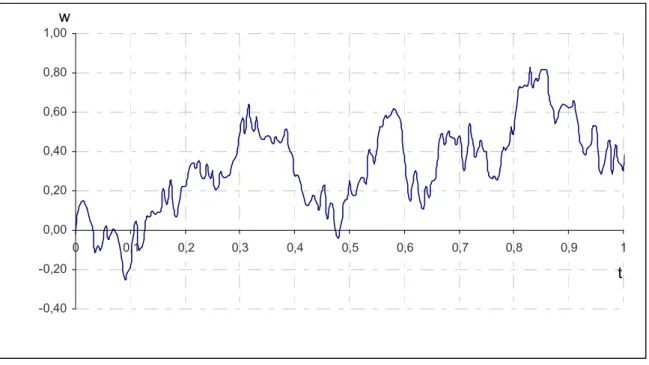
The Wiener process: This describes a variableW, sometimes referred to as Brownian
motion, whose change is measured over the interval t such that its mean change is zero and
23 For a general introduction please see Christopher, 1996, pp:151-159 and see Hull ,1997, pp:216-229 to
variance proportional to t . The change in the variable Wis W
( )
t ~ N(
0, t)
wheret
W = with ~ N
( )
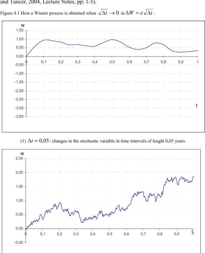
0,1 . In addition, the increments W are independent across time because winner process is a markov process24 (Hull, 1997, p: 218-219; Jorion, 2003, p.84 and Tuncer, 2004, Lecture Notes, pp: 1-5).Figure 4.1 How a Wiener process is obtained when t '0 in W = t .
-3,50 -3,00 -2,50 -2,00 -1,50 -1,00 -0,50 0,00 0,50 1,00 1,50 0 0,1 0,2 0,3 0,4 0,5 0,6 0,7 0,8 0,9 1 t w
(1) t =0,05: changes in the stochastic variable in time intervals of lenght 0,05 years.
-0,50 0,00 0,50 1,00 1,50 2,00 2,50 0 0,1 0,2 0,3 0,4 0,5 0,6 0,7 0,8 0,9 t1 w
(2) t =0,005: changes in the stochastic variable in time intervals of lenght 0,005 years.
Table 4.1 (continued) -0,40 -0,20 0,00 0,20 0,40 0,60 0,80 1,00 0 0,1 0,2 0,3 0,4 0,5 0,6 0,7 0,8 0,9 1 t w
(3) t =0,003: changes in the stochastic variable in time intervals of lenght 0,003 years.
The Generalized Wiener process: This describes a variable X built up from a Wiener processW, which has an expected drift rate of a and a variance rate of ( )b2( Hull, 1997, p.221). bdW adt dX = + 4.1 dt b adt dX = + 4.2 where
(
( )
2)
, ~ adt bdX N dW . The equation 4.1 consists of two parts deterministic
component and stochastic component. A particular case is the martingale, which is a zero drift stochastic process, a=0. This has the convenient property that the expectation of a future value is the current value (Hull, 1997, pp: 219-222,; Jorion, 2003, p.84 and Tuncer, 2004, Lecture Notes, pp: 5-6).
The Ito process: This describes a generalized Wiener process, whose trend and volatility
depend on the current value of the underlying variable and time (Hull, 1997, pp: 226-227 and Jorion, 2003, pp: 226-227).
( ) ( )
t a x t dt b( )
x t dWSo far, it has been explained a continuous variable, a continuous time stochastic process of a risk factor. The crucial point is to choose a particular stochastic model for the behavior of a price level and then to calculate it by using Ito’s lemma. But what models should be use? The answer depends on the instrument whose risk factor it wish be modeled.
ii. Geometric Brownian Motion
For stock prices and currencies a commonly used model is the Geometric Brownian Motion (GBM). The GBM can be shown as
( )
t S( )
t dt S( ) ( )
t dW tdS =µ + 4.4
where S is the current price of the stock, dS is the change in the stock price, µ is the expected rate of return (drift), is the volatility of S ,dW = wiener increment = dt ,
is the standard normal distribution. This model assumes that the innovations in the asset price are uncorrelated over time (Tuncer, Ruhi, 2004, Lecture Notes, pp: 26-28).
The stochastic process of pricing stock prices and currencies require two parameters estimation : the drift µ and the volatility . Kim, Malz and Mina (1999) have shown that “mean forecasts for horizons shorter than three months are not likely to produce accurate predictions for future returns. In fact, most forecasts are not likely to predict the sign of returns for a horizon shorter than three months. In addition, since volatility is much larger than the expected return at short horizons, the forecasts of future returns are dominated by the volatility estimate . In other words, if it is being concerned with short horizons, using a zero expected return assumption is as good as any mean estimate” (As cited in Mina and Xiao, 2000). Hence, from this point view, it will been made the explicit assumption that the expected return is zero.
The next question is how to estimate the volatility . Three different models are generally used to estimate volatility: Historical Average (HA), Exponentially Weighted Moving Average (EWMA) and Generalized Autoregressive Conditional Heteroscedastic (GARCH) model.
The process (4.4) is geometric because the trend and volatility names are proportional to the current value ofS.This is normally the case for stock prices, for which rates of returns come into view to be more stationary than the dollar returns. It is also used for currencies (Jorion, 2003, p. 84).
This model is particularly important because it is the underlying process for the Black-Scholes formula25. The important feature of this distribution is the fact that the volatility is proportional toS. This guarantees that the stock price will remain positive. In addition, when the stock price falls, its variance decreases. This makes it impossible to experience a large downmove that may drive the price into negative values (Jorion, 2003, p. 85).
.
Using a logarithm transformation and applying the Ito’s lemma26, it can be reach the equation for the risk factor simulation which can be shown as:
( )
(0) exp 2( )
2
S t =S (µ )t+ W t 27 4.5
The model is based on a normal distribution of the underlying risk factor returns which is the same thing as saying that the underlying prices themselves are lognormally distributed. This is an important result. If stock prices displays a geometric Brownian motion, their distribution is log normal. A lognormal distribution is the right skewed distribution. The lognormal distribution permits for a stock price distribution between zero and infinity (i.e. no negative prices) and has an upward bias (representing the fact that a stock price can only drop 100% but can rise by more than 100%)
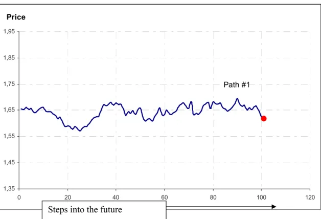
The equation 4.4 can be repeated as often as needed. Define K as the number of replications. Figure 4.2 displays one trial which leads to final value
( )
S TK. This generates a distribution of simulated prices( )
S T. With just one stepn=1, the distribution must be25 For the derivation see Tuncer, 2004, FEC 552, Lecture Notes, pp: 29-37. 26 Tuncer, 2004, FEC 552, Lecture Notes, pp: 5-26.
27
normal. As the number of steps n grows large, the distribution attends to a lognormal
distribution.
Figure 4.2 Simulating price path
Price 1,35 1,45 1,55 1,65 1,75 1,85 1,95 0 20 40 60 80 100 120 Path #1
Figure 4.3 Simulating price paths
Price 1,35 1,45 1,55 1,65 1,75 1,85 1,95 1 11 21 31 41 51 61 71 81 91 101
Steps into the future
iii. Simulating yields
Although the GBM process is generally used for stocks and currencies, it cannot used by fixed-income products such as bond prices and commodities which presents mean reversion28. Such process is inconsistent with the GBM process, which presents no such mean reversion29.
The dynamics of interest rates r t can be modeled by
( )
( )
(
( )
)
( ) ( )
dr t =* + r t dt+ r t dW t 4.6
where dW t is the usual Wienner process. Here, it is assumed that
( )
0&*<1,+ -0, -0. Jorion (2003) explains this Markov’features as the following:.1. First, it presents mean reversion to a long-run value of + . The parameter * manages the speed of mean reversion. When the current interest rate is high, i.e.r t
( )
f , the model has a negative drift + * +(
r t( )
)
toward+ . Conversely, lowcurrent rates create with a positive drift.
2. The second feature is the volatility process. This class of model includes the
Vasicek model when. =0. Changes in yields are normally distributed because
ris a linear function of z. This model is particularly useful because it leads to closed-form solutions for many fixed-income products. However, the problem is that it may allow negative interest rates because the volatility of the change in rates does not depend on the level.
Equation is more general because it includes a power. of the yield in the variance function. With. =1, the model is the lognormal model. This implies that the rate of change in the yield has a fixed variance. Thus, as with the GBM model, smaller yields lead to smaller movements, which makes it impossible the yield will drop below zero.
28 See Zangari, 1996, pp: 107-117.
With. =0,5, this is the Cox, Ingersoll, and Ross (CIR) model. Ultimately, the choice of the explanatory . is an empirical issue. Recent research has shown that . =0,5 provides a good fit to the data.
Using a logarithm transformation and applying the Ito’s lemma, it can be reached the equation for the interest rate simulation which can be shown as:
( )
( )
( ) ( )
) ) ( ( =b b r t/
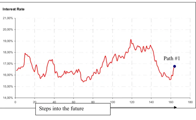
atdW t t r t 0 exp exp 30 4.7Thus, at low values of the interest rate, the standard deviation becomes close to zero, cancelling the effect of the random shock on the interest rate. Consequently, when the interest rate gets close to zero, its evolution becomes dominated by the drift factor, which pushes the rate upward (Hull, 2003, p.100).
The equation 4.7 can be repeated as often as needed. Define K as the number of replications. Figure 4.4 displays one trial which leads to final value
r
TK. This generates a distribution of simulated pricesr
T.Figure 4.4 Simulating interest rate path
Interest Rate 14,00% 15,00% 16,00% 17,00% 18,00% 19,00% 20,00% 21,00% 0 20 40 60 80 100 120 140 160 180
30 Tuncer, 2004, FEC 552, Lecture Notes, pp: 27-29
Steps into the future
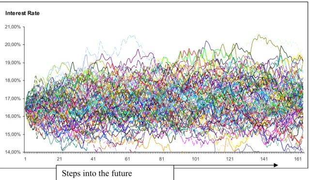
Figure 4-5 Simulating interest rate paths Interest Rate 14,00% 15,00% 16,00% 17,00% 18,00% 19,00% 20,00% 21,00% 1 21 41 61 81 101 121 141 161
It has already been mentioned the content of the Monte Carlo simulation approach. Now is the time to make up for the steps of calculation VaR.
4.2 Applying Monte Carlo Simulation VaR Methodology
Linsmeier and Pierson (1996), explains computation of VaR for a single instrument portfolio using Monte Carlo simulation approach in five steps:
1. The first step is to identify the basic risk factors, and to obtain a formula expressing the mark-to-market value of the position in terms of the risk factors subjecting to current price level Pcpl. That is,
cpl k S P ,trf i log = e Prfi, P P ,t-1 rf i 4.8
2. The second step is to determine a specific distribution for risk factor returns and to estimate the parameters of that distribution.
3. The next step is to generate generator hypothetical values of risk factor returns bu using pseudo-random. Then these hypothetical risk factors are used to calculate hypothetical mark-to-market portfolio values. Hypothetical daily profits and losses are calculated from each of the hypothetical portfolio values,
4. The last to steps are the same as in historical simulation. The mark-to-market profits and losses are ordered from the largest loss to lowest one. The value at risk is the loss which is equaled or exceeded p% of the time.
Using the probability of p percent, this is the value at risk for GBM model. That is,
(
)
( )
{
}
{
}
(
)
1 2 (0) exp 1 ,1 , 1 2 ,1 & 1 1 & ,1 m S t W t NV percentile P e p VaRp t cpl i i m percentile P Li p m percentile P LT m i p m i µ 0 + × = "" ( ) # # + $ % $ % = = "" & # # $ % $ %(
)
( )
1 1 & p F P L k = =Using the probability of p percent, this is the value at risk for CIR model. That is,
(
)
( )
( ) ( )
{
}
{
}
(
)
exp exp 1 ,1 , 1 0 1 ,1 & 1 1 1 & 1 m t b b r t at dW t percentile NV p VaRp t Pcpl e i m percentile P Li i p m percentile P LT m i m i ( / ) = "" × # # + ( ) $ % = $ % = = = & =(
)
( )
,1 1 1 & p p F P L k "" # # $ % $ % = =The model explained above applies to a single risk factor. As it will be illustrated, the model can be generalized to describe the dynamics of multiple risk factors.
4.3 Monte Carlo Simulation VaR with Multiple Sources of Risk
It is now turned to the more general case of simulations with many sources of n financial risk factors. According to Linsmeier and Pearson (1996), such a case requires only that a
bit of additional work to be performed in three of the steps, just as with historical simulation.
1. In step 1, there are likely to be many more risk factors. These factors must be identified, and pricing formulas expressing the instruments` values in terms of risk factors must be obtained.
2. In step 2, the joint distribution of returns scenarios for all of the risk factors must be determined by using standard normal variables. To the this, a matrix is needed which requires n independent standard normal variables. The important thing is the choice of a matrix is not unique.
Two popular methods for a matrix are the Cholesky decomposition and the Singular
Value decomposition (SVD)31. Mina and Xia (2001) states in his paper one important difference between these decompositions that the Cholesky algorithm cannot provide a decomposition when the covariance matrix is not positive definite. A non-positive definite covariance matrix requires a situation where at list one of the risk factors is repetitive, meaning that the repetitive risk factor can be reproduced as a linear combination of the other risk factors. This situation generally corresponds when the number of days used to calculate the covariance matrix is smaller than the number of risk factors (Mina and Xiao, 2001, p.19). The correlation structure can be protected in the process of simulation by “Cholesky Factorization”. The process requires factorizing the covariance matrix into a lower triangular and an upper triangular matrix. The critical point here is that the covariance matrix should be positive definite and symmetric in order to be decomposed. (Zangari, 1996, p.253-255).
According to Jorion (2003),
• The simulation can be firstly adapted by drawing a set of independent variables1 ,
• Then it is adapted by transforming them into correlated variables . As an example for two factors : It can be written
1=11
(
2)
1/ 2 2=211+ 1 2 12Here, 2 is the correlation coefficient between the variables . Due to unit variance and uncorrelated 1 , it is verified that the variance of s 2is one, as required. That is,
( )
2( )
(
2)
1/ 2 2( )
2(
2)
2 =2 11 +(1 2 ) 12 =2 + 1 2 =1
V V V ,
In addition, the correlation between 1 and 2 is defined by
(
)
(
(
2)
1/ 2)
(
)
1, 2 = 11, 211+ 1 2 12 =2 1 11, 2 =2
Cov Cov Cov
Defining as the vector of values, it is verified that the covariance matrix of is
( )
( )
(
)
(
)
( )
2 1 1 2 2 1 2 2 , 1 1 , Cov p V R p Cov = = =Note that this covariance matrix, which is the expectation of squared deviation from the mean, can be written as
( )
(
( )
)
(
( )
)
'( )
'V =E( E × E )=E ×
because the expectation of is zero.
3. In Step 3, similar to historical simulation, to reflect accurately the correlations of market rates and prices it is necessary that the mark-to-market profits and losses on every instrument be computed
4. Then P&L are summed for each day, before they are ordered from highest profit to lowest loss in Step 4.
Let us assume that there is n factors denoted by S t and
( )
j r t j( )
j=1,...,n. If the factors( )
jS t and r t
( )
jare independent, the processes can be performed independently for each variable, respectively. For the GBM model,( )
j( )
j( )
j( )
jwhere the standard normal variables are independent across time.This means that the stock price can be written as
( )
(0) exp 2( )
2 µ = ( j) + j j j j S t S t W t 4.10For the interest rate model,
( )
j=* +(
( )
j)
+( )
j( )
jdr t r t dt r t dW t 4.11
where the standard normal variables are independent across time.This means that the interest rate simulation can be written as
( )
exp( )
exp( ) ( )
0 ( ) = / ( ) j j j t r t b b r t at dW t 4.12It is seen that the evaluation of stock price over time are almost identical for a single or multiple risk factors. The only difference is that if there are more than one risk factors, the correlation between returns on the various risk factors is taken into account.
Now, portfolio P&L can be ordered and then VaR can be read off by expressing the above process into blove formula to get the kth ordered P&L with the given confidence level at the defined sample histogram for GBM as the following:
(
)
( )
{
}
{
}
(
)
1 2 (0) exp 1 ,1 , 1 2 1 1 ,1 & 1 1 1 & 1 m n S t W t percentile NV j j p VaRp t Pcpl e j j j i m percentile P Li i p m percentile P LT m m i µ + = "" × ( ) # # + = $ % = $ % = = = =(
)
( )
,1 1 1 & i p p F P L k & "" # # $ % $ % = =where k =
(
1 p)
m. Thus, VaR is simply the lower percentile of the portfolio P&L distribution.Using the probability of p percent, the value at risk for CIR model is the following:
(
)
( )
( ) ( )
{
}
{
}
exp exp 1 ,1 , 1 0 1 1 ,1 & 1 1 1 1 m t n b b r t at dW t percentile NV p VaRp t Pcpl e j j j i m percentile P Li i p m percentile T m i ( / ) = "" × # # + ( ) = $ % = $ % = = = =(
)
(
)
( )
,1 & 1 1 & i p P L m p F P L k & "" # # $ % $ % = =It has already been mentioned the process of calculating VaR by using the MCS approach, but so far the concept has not been precise regarding its pros and cons. Now is the time to make up for that.
4.4 Advantages & Disadvantages Advantages
• The independence between the distributional assumptions and the specific portfolio pricing functions allows flexibility to examine risk (Mina, Jorge and Xiao J., Yi, 2001, p.19).
• It is model-based approach.
• It accounts for a wide range of risks, including non-linear price risk, volatility risk and even model risk.
• It can incorporate time variation in volatility, fat tails and extreme scenarios.
Disadvantages
• The biggest drawback of this method is its computational cost.
• The generation of the scenarios is based on random numbers drawn from a theoretical distribution, which is inconsistent to the empirical distribution of most asset returns (Barone-Adesi, Giannopoulos and Vosper, 2000, p.3).
• During market crises, monte Carlo simulation is likely to underestimate the possible losses when most historical correlations tend to increase rapidly (Barone-Adesi, Giannopoulos and Vosper, 2000, p.3).
• When a large number of scenarios is generated, simulation tends to slow (Barone-Adesi, Giannopoulos and Vosper, 2000, p.3).
Thus, overall, this method is probably the most comprehensive approach to measuring risk if modeling is done correctly.
5 WEIGHTED HISTORICAL SIMULATION VaR METHODOLOGY
An interesting variation of the historical simulation methodology is the weighted historical simulation methodology (called hybrid methodology, as well). This method is supported by Boudoukh, Richardson and Whitelaw (1998). This approach combines RiskMetrics and historical simulation methodologies by applying exponentially declining weights to past returns.
This chapter introduces Weighted Historical Simulation (WHS) VaR Methodology. Section 3.1 works in a simple case with just one source of risk. Section 3.2 shows how to apply these methods to construct VaR . Then multiple sources of risk are considered in Section 3.3.
5.1 Weighted Historical Simulation VaR with One Source of Risk
It has been discussed the HS VaR Methodology approcah regarding the choice of sample size, m. All observations older than m get zero weight, and all observations more recent than m get equal weight. That is,
1/ 0 0 m if j m w j=" else& < $ 5.1 32
This is an extreme choice for a “weighting function” for the observations (Andrew, 2006, Lecture Notes, pp: 163-164). If m is too small, then there are not enough observations in the left tail to calculate VaR. If m is too large, then the VaR will not be sufficiently responsive to the most recent returns (Christoffersen, 2003, p.103). An alternative might assign higher weight to more observations, and a lower weight to older observations, which the weights smoothly declining in the age of the observations. Such an approach is c “weighted historical simulation” (WHS) (Andrew, 2006, Lecture Notes, p. 163).
WHS is implemented as follows:
m is the sample of observations to use and is a smoothing parameter inside (0,1). An exponentially declining weighting function is used:
(
1)
(
1)
0 0 j m if j m w j else & < =" $ 5.2 3332 See Andrew, 2006, AF365, Lecture Notes, p. 163 and Christoffersen, 2003, p.101. 33 See Andrew, 2006, AF365, Lecture Notes, p. 164 and Christoffersen, 2003, p.103.
This function is such that the weights decline exponentially as j increases, and that 1 0 1 m j j=
w
= .By weighting recent observations more heavily than older observations more of the time-varying nature of the distribution of returns is captured. In addition, since observations near m have to weight, the choice of m becomes less critical. However the choice of
can be very important. Values of =0.99 or =0.95 have been used in past studies (Andrew, 2006, Lecture Notes, pp: 163-164).
The weighted empirical cdf is
( )
rw
{
r
r}
F
t j m j j t = & = + 1 1 0 1 5.3 34and the VaR forecast based on the weighted empirical cdf is again obtained by inverting the function
(
p)
F
VaR
HSt+ = t+ 1 1 1 1 , 5.4 35which is obtained in practise by assigning weights, w j, to each observation in the sample,
rt j, then sorthing these observations, and then finding the observation such that the sum of the weights assigned to returns less than or equal that observation is equal to
(
1 p)
(Andrew, 2006, Lecture Notes p.164).It has already been mentioned the content of the WHS-VaR-Methodology. Now is the time to make up for the steps of calculation VaR.
5.2 Applying Weighted Histrical Simulation
Boudoukh, Richardson, and Whitelaw (1998) explain the computation of VaR for a portfolio using WHS VaR Mathodology as the following steps:
1. Risk factors: The first step is to identify n risk factors rf i, with i=1,...,n.
34 See Andrew, 2006, AF365, Lecture Notes, p. 164 and Christoffersen, 2003, p.103. 35 Oomen, 2006 , AF365, Lecture Notes, p. 23.
2. Data: The next step is to collect historical values of n risk factors for the last
determined period.
3. Return: Then their returns are obtained and each return is assigned its corresponding
weight.
4. Secanarios for risk factors price levels: This is the key step which attempts to obtain a
formula Prfi expressing the mark-to-market value of the position in terms of each risk factor
subjecting to current price level Pcpl.
cpl k S P ,trf i log = e Prfi, P P ,t-1 rf i 4.5
where i=1,...,n. That is, if there is an instrument in a position and it contains n risk factors , the scenarios of each future are obtained by expressing prices in a function of logarithmic returns of each risk factor. The current portfolio is subjected to the percentage changes in risk factors and prices experienced on each of determined period.
5. PV of instrument: The present value of an instrument is expressed as a fuction of the n
risk factors rf i, with i=1,...,n
6. Portfolio P&L: Calculating the daily profits and losses that would occur if comparable
daily changes in the risk factors are experienced and the current portfolio is marked-to-market.
7. Portfolio P&L: The next step is to order the mark-to-market profits and losses and
weights in descending order by P&L. Unlike HS VaR Methodology, WHS VaR Methodology assignes weights to each observation in the sample by weighting recent observations more heavily than older observations then sorting these observations.
Table 5.1 WHS -VaR calculation steps with one source of risk
Data Return (R) Scenarios (S) PV P&L
t P 1 t P t-1 1,t-1 t P =log r P t-1 t-1= r S Pcple PVt-1 P&Lt-1 2 t P t-2 1,t-2 t-1 P = log r P t-2 t-2= r S Pcple PVt-2 P&Lt-2 . . . . . . . . . . t m P r1,t-m St-m=Pcplert-m PVt-m P&Lt-m
Finally, the loss which is equaled or exceeded p percent of the time is selected. Using the probability of (1-p) percent, this is the value at risk. This processes can be shown analytically as the following:
(
)
{
}
{
}
(
)
(
)
(
)
{
}
, log 1 ,1 , 1 , 1 1 ,1 & 1 1 1 1 & ,1 1 m Prf i t percentile NV p VaRp t Pcpl e P t rf i i m percentile P Li i p m j m percentile P LT m i p i = "" × # # + $ % = $ % = = = " & # = $ %(
)
1 1 & ( ) p F P L k = =It has been shown that the steps of WHS VaR Methodology to calculate VaR is similar to HS VaR Methodology except that WHS VaR Methodology assignes weights to each observation in the sample by weighting recent observations more heavily than older observations.
5.3 Weighted Historical Simulation VaR with multiple sources of risk
It is now turned to the more general case of simulations with many sources of financial risk. This section introduces Weighted Historical Simulation VaR Methodology with multiple sources of risk which requires an additional work.
Let us assume that there is m positions denoted by &P L j , j=1,...,m. After summing profits and losses for each position for each day, they are ordered from the highest profit to lowest loss.
Table 5.2 WHS-Portfolio P&L with multiple source of risk
Portfolio P&L
, ,
n
P & L1,t + P & L2,t + ...+ P & L n,t P&L P&Lp t i t i=1 = = , , n
P & L1,t-1+ P & L2,t-1+ ...+ P & Ln,t-1 P&L P&Lp t-1 i t-1 i=1 = = , , n
P & L1,t-2 + P & L2,t-2 + ...+ P & Ln,t-2 P&L P&Lp t-2 i t-2 i=1 = = , , n
P & L1,t-3+ P & L2,t-3 + ...+ P & Ln,t-3 P&L P&L p t-3 i t-3 i=1 = = . , , n
P & L1,t-m+ P & L2,t-m + ...+ P & Ln,t-m P&L P&L p t-m i t-m
i=1
= =
Now, portfolio P&L can be ordered and then VaR can be read off by expressing the above process into blove formula to get the kth ordered P&L with the given confidence level at the defined sample histogram or sample inverse cumulative distribution function as the following:
, log 1 ,1 , 1 , 1 1 1 ,1 & 1 1 m Prf t n i percentile NV p VaRp t Pcpl e P t rf i i i m n percentile P Li p i percentile i 0 = "" × # # + $ = % = $ % = "" # # = $ % = $ % =
(
1)
(
1)
1(
&)
,1 1 1 1(1 ) & ( ) m m j m P LT j i p J p F P L k & "" # # = $ % = $ % = =Thus, VaR is simply the lower percentile of the portfolio P&L distribution. It is seen that VaR caluculation can be performed without using standard deviation or correlation forecasts. (Longerstaey,1996, p.6).
It has already been mentioned the process of calculating VaR by using the HS approach, but so far the concept has not been precise regarding its pros and cons. Now is the time to make up for that.
5.4 Advantages & Disadvantages
Christoffersen36 (2003) explains the prons and cons of this methodology in the following:
Advantages:
• Like HS VaR Methodology, WHS VaR Methodology does not require estimation and thus maintains the ease of implementation .
• Unlike HS VaR Methodology, WHS VaR Methodology sorts changes in the value of the portfolio by weighting recent observations more heavily than older observations, which provides consistency with today’s market conditions.
• Unlike HS VaR Methodology, WHS VaR Methodology makes the choice of m somewhat less crucial.
Disadvantages:
• No guidance is given on how to choose .