FAST MULTIPOLE METHOD FOR THE
SOLUTION OF ELECTROMAGNETIC
SCATTERING PROBLEMS
a thesis
submitted to the department of electrical and
electronics engineering
and the institute of engineering and sciences
of bilkent university
in partial fulfillment of the requirements
for the degree of
master of science
By
¨
Ozg¨ur Salih Erg¨ul
June 2003
I certify that I have read this thesis and that in my opinion it is fully adequate, in scope and in quality, as a thesis for the degree of Master of Science.
Assoc. Prof. Dr. Levent G¨urel (Supervisor)
I certify that I have read this thesis and that in my opinion it is fully adequate, in scope and in quality, as a thesis for the degree of Master of Science.
Prof. Dr. Ergin Atalar
I certify that I have read this thesis and that in my opinion it is fully adequate, in scope and in quality, as a thesis for the degree of Master of Science.
Asst. Prof. Dr. Vakur B. Ert¨urk
Approved for the Institute of Engineering and Sciences:
Prof. Dr. Mehmet Baray
ABSTRACT
FAST MULTIPOLE METHOD FOR THE
SOLUTION OF ELECTROMAGNETIC
SCATTERING PROBLEMS
¨
Ozg¨ur Salih Erg¨ul
M.S. in Electrical and Electronics Engineering
Supervisor: Assoc. Prof. Dr. Levent G¨urel
June 2003
The fast multipole method (FMM) is investigated in detail for the solution of elec-tromagnetic scattering problems involving arbitrarily shaped three-dimensional conducting surfaces. This method is known to reduce the computational com-plexity and the memory requirement of the solution without sacrificing the accu-racy. Therefore, it achieves the solution of large problems with less computational resources compared to the other traditional solution algorithms. However, the ex-pected efficiency of the FMM may not be obtained unless the appropriate choices of the components are made. The types of the employed integral equation, it-erative algorithm, and preconditioning technique directly affect the efficiency of the implementations. Performances of these components are also related to each other, and their simultaneous optimization creates a challenging task in the de-sign of an efficient solver.
Keywords: Fast multipole method (FMM), electromagnetic scattering, integral equations, iterative algorithms, preconditioning techniques.
¨
OZET
ELEKTROMANYET˙IK SAC
¸ INIM PROBLEMLER˙I ˙IC
¸ ˙IN HIZLI
C
¸ OKKUTUP Y ¨
ONTEM˙I
¨
Ozg¨ur Salih Erg¨ul
Elektrik ve Elektronik M¨uhendisli˘gi B¨ol¨um¨u Y¨uksek Lisans
Tez Y¨oneticisi: Do¸c. Dr. Levent G¨urel
Haziran 2003
Geli¸sig¨uzel ¸sekilli ¨u¸c boyutlu iletken y¨uzeyleri i¸ceren elektromanyetik sa¸cınım problemlerinin ¸c¨oz¨um¨u i¸cin hızlı ¸cokkutup y¨ontemi (HC¸ Y) incelenmi¸stir. Bu y¨ontemin, hesapsal karma¸sıklı˜gı ve bellek gereksinimini, ¸c¨oz¨um¨un dogrulu˜gundan taviz vermeden d¨u¸s¨urd¨u˜g¨u bilinmektedir. B¨oylece, b¨uy¨uk problemlerin ¸c¨oz¨um¨u geleneksel ¸c¨oz¨um algoritmalarına g¨ore bilgisayar kaynaklarının daha az kullanı-mıyla yapılabilmektedir. ¨Ote yandan, HC¸ Y’nin beklenen verimlili˜gi, bile¸senleri uygun se¸cilmedi˜gi s¨urece elde edilemeyebilir. Kullanılan integral denklemi, ite-ratif algoritma ve preconditioning tekni˜gi uygulamanın verimlili˜gini do˜grudan etkiler. Bunların kullanımının birbirine ba˜glı olmasından dolayı, verimli bir ¸c¨oz¨uc¨un¨un tasarımı zorlu bir i¸se d¨on¨u¸smektedir.
Anahtar kelimeler: Hızlı ¸cokkutup y¨ontemi (HC¸ Y), elektromanyetik sa¸cınım, in-tegral denklemleri, iteratif algoritmalar, preconditioning teknikleri.
ACKNOWLEDGMENTS
I gratefully thank my supervisor Dr. Levent G¨urel for his supervision, guidance, and suggestions throughout the development of this thesis. I would also like to express my deepest gratitude to him for supporting my studies on the computa-tional electromagnetics.
I also thank Prof. Dr. Ergin Atalar and Dr. Vakur B. Ert¨urk for reading and commenting on this thesis.
I also thank Prof. Dr. Ayhan Altınta¸s for commenting on this thesis.
I also thank all undergraduate and graduate students of Bilkent Computational Electromagnetics Laboratory for their cooperation and accompaniment in my studies.
Contents
1 Introduction 1
1.1 Motivation . . . 1
1.2 Historical Background . . . 2
1.3 Contributions . . . 5
1.4 Simulation Environment and Computational Resources . . . 6
2 Integral Equations 7 2.1 Electric-Field Integral Equation . . . 7
2.2 Magnetic-Field Integral Equation . . . 8
2.2.1 Radiation Integral . . . 9
2.2.2 Derivation by Using Interior Boundary Condition . . . 12
2.3 Combined-Field Integral Equation . . . 13
2.4 Method of Moments . . . 14
2.4.1 Geometry Modelling and Meshing . . . 16
2.4.2 Triangular Rooftop Basis Functions . . . 19
3 MOM Implementations with the EFIE 22 3.1 Formulation . . . 22
3.2 Singularity Extraction . . . 27
3.3 Evaluation of Impedance-Matrix Elements . . . 32
3.4 Numerical Evaluation of Integrals . . . 33
3.4.2 Adaptive Integration: Method 2 . . . 36
3.5 Excitation . . . 40
3.5.1 Plane-Wave Excitation . . . 40
3.5.2 Delta-Gap Excitation . . . 41
3.5.3 Current Sources . . . 42
3.6 Computational Analysis of the MOM . . . 43
3.7 RCS Calculations for RWG Basis Function . . . 44
4 MOM Implementations with the MFIE and the CFIE 46 4.1 MFIE-MOM Implementation with RWG Testing Function . . . . 47
4.1.1 Formulation . . . 48
4.1.2 Singularity Extraction . . . 50
4.1.3 Evaluation of the Impedance-Matrix Elements . . . 56
4.1.4 Singularity Extraction for Outer Integrals . . . 63
4.1.5 Numerical Integration of Inner and Outer Integrals . . . . 66
4.1.6 Excitation . . . 67
4.2 MFIE-MOM Implementation with Point Testing Functions . . . . 67
4.2.1 Formulation . . . 68
4.2.2 Evaluation of the Impedance-Matrix Elements . . . 70
4.3 CFIE-MOM Implementation with RWG Basis and Testing Functions 75 4.4 CFIE-MOM Implementation with Point Testing Function for the MFIE . . . 76
4.5 Results . . . 76
5 FMM Implementations 86 5.1 Theory of the FMM . . . 87
5.1.1 Factorization of the Green’s Function . . . 87
5.1.2 Calculation of an Interaction . . . 88
5.1.4 Truncation Number . . . 95
5.1.5 Integration Points . . . 98
5.1.6 Computational Analysis of the FMM . . . 99
5.2 FMM Implementation with RWG Basis Functions . . . 102
5.3 Results . . . 103
5.3.1 Accuracy of the FMM Implementations . . . 104
5.3.2 Efficiency of the FMM Implementations . . . 104
6 Iterative Methods and Preconditioning Techniques 109 6.1 Iterative Solution of the Linear Systems . . . 110
6.1.1 Bi-Conjugate Gradient (BiCG) Algorithm . . . 111
6.1.2 Conjugate Gradient Squared (CGS) Algorithm . . . 115
6.2 Preconditioning Techniques . . . 116
6.2.1 Types of Preconditioners . . . 117
6.2.2 Comparisons of Preconditioners and Iterative Solvers . . . 121
6.3 Comparisons of the Integral Equations . . . 122
6.3.1 Efficiency of the FMM for Different Formulations . . . 124
6.3.2 Choice of α in the CFIE . . . 126
6.4 Effect of Initial Guess on the Convergence . . . 126
6.5 Multiple Excitations . . . 127
7 MLFMA Implementations 132 7.1 Evaluation of Interactions with the MLFMA . . . 133
7.1.1 Aggregation in the MLFMA . . . 133
7.1.2 Translation in the MLFMA . . . 139
7.1.3 Disaggregation in the MLFMA . . . 140
7.2 Clustering and Structure of the MLFMA . . . 146
7.3 Computational Analysis of the MLFMA . . . 148 7.3.1 Computational Analysis of Aggregation and Disaggregation 149
7.3.2 Computational Analysis of Translation . . . 150
7.4 Results . . . 152
7.4.1 Accuracy of the MLFMA Implementations . . . 153
7.4.2 Efficiency of the MLFMA Implementations . . . 153
8 Conclusion 155
Bibliography 158
List of Figures
2.1 Observation point approaching a smooth portion of the surface
from outside. . . 10
2.2 Surface models of various closed geometries with triangular meshing. 17 2.3 Surface models of various open geometries with triangular meshing. 18 2.4 RWG function defined on the triangular domains. . . 19
3.1 RWG function does not have current flow across its boundaries. . 24
3.2 Location of the basis and testing triangles after the coordinate transformation. . . 26
3.3 Source triangle on the x-y plane and projection of the observation point. . . 28
3.4 Geometric variables introduced to express the results of analytical integrals. . . 29
3.5 Different cases for the projection of the observation point. . . 31
3.6 Adaptive integration method 1. . . 34
3.7 Function to be integrated on the triangular domain. . . 36
3.8 Integration points taken by the first adaptive method to evaluate the integral of the function shown in Figure 3.7 . . . 37
3.9 Adaptive integration method 2. . . 38
3.10 Integration points taken by the second adaptive method to evalu-ate the integral of the function shown in Figure 3.7 . . . 39
3.12 Current sources defined with the RWG functions. . . 42 3.13 Corresponding physical equivalences for the current sources shown
in Figure 3.12. . . 43 4.1 Limit cases for observation points approaching the basis triangle. . 52 4.2 Observation points approaching the edge at different angles. . . . 54 4.3 Magnitude of the integral I =RS
jdr
0zzfˆ m3(R) for the scenario in Figure 4.2. . . 54 4.4 Interaction between the neighboring basis and testing triangles. . 61 4.5 Limit case as the observation point approaches the edge of the
basis function. . . 62 4.6 Second coordinate transformation used to annihilate the
singular-ity of the outer integral. . . 64 4.7 Point testing functions. . . 68 4.8 Point testing function approaching the center of the edge of the
basis function from outside. . . 70 4.9 Point testing function approaching the edge of the basis triangle. . 71 4.10 The testing function residing on one of the edges of the basis
tri-angle, on which the basis function is not defined. . . 73 4.11 Models of a sphere having a radius of 0.3 m with mesh sizes (a)
6 cm, (b) 5 cm, (c) 4 cm, and (d) 3 cm. . . 79 4.12 RCS values obtained by the EFIE-MOM implementation for a
sphere with a radius of (a) 0.5 λ, (b) 0.6 λ, (c) 0.75 λ, and (d) 1.0 λ. 81 4.13 RCS values obtained by the MFIE-MOM implementation using
point testing functions for a sphere with a radius of (a) 0.5 λ, (b) 0.6 λ, (c) 0.75 λ, and (d) 1.0 λ. . . . 82 4.14 RCS values obtained by the MFIE-MOM implementation using the
RWG functions and Galerkin method for a sphere with a radius of (a) 0.5 λ, (b) 0.6 λ, (c) 0.75 λ, and (d) 1.0 λ. . . . 83
4.15 RCS values obtained by the CFIE-MOM implementation using the RWG functions and Galerkin method for a sphere with a radius of
(a) 0.5 λ, (b) 0.6 λ, (c) 0.75 λ, and (d) 1.0 λ. . . . 84
4.16 RCS values obtained by the EFIE, the MFIE, and the CFIE for-mulations for a sphere with a radius of 0.8 λ. The MFIE suffers from the internal resonance problem. . . 85
5.1 Dividing r − r0 into segments. . . 89
5.2 Clustering of basis and testing functions provides a single transla-tion between the clusters. . . 91
5.3 Aggregation process in basis clusters. . . 92
5.4 Translation from a basis cluster to testing clusters. . . 93
5.5 Disaggregation process in testing clusters. . . 94
5.6 Magnitude of the imaginary part of the Hankel function, h(1)l (x) with respect to l for different values of x. . . . 96
5.7 Values of L obtained with the formula given in Equation (5.24) and direct test of Equation (5.8) for an accuracy of three digits. . 97
5.8 Angular integration points for L = 5. . . . 99
5.9 RCS values obtained by the EFIE-FMM implementation using the RWG functions and the Galerkin method for a sphere having a radius of (a) 0.75 λ, (b) 1.0 λ, (c) 1.5 λ, and (d) 2.0 λ. . . 107
5.10 RCS values obtained by the CFIE-FMM implementation using the RWG functions and the Galerkin method for a sphere having a radius of (a) 0.75 λ, (b) 1.0 λ, (c) 1.5 λ, and (d) 2.0 λ. . . 108
6.1 General form of an iterative solution. . . 110
6.2 Pseudocode of a general BiCG algorithm for complex systems. . . 113
6.3 Pseudocode of the reduced form of the BiCG algorithm for complex symmetric systems. . . 115
6.4 Pseudocode of the general CGS algorithm for complex systems. . 116
6.5 Self-cluster interactions in the impedance matrix of an 72-unknown problem. . . 119
6.6 Self-cluster interactions in the impedance matrix of an 72-unknown problem after the renumbering operation. . . 120
6.7 Plots of the residual versus the iteration number for different types of preconditioners implemented with CGS and BiCG for the solu-tion of (a) 1302-unknown, and (b) 8364-unknown scattering prob-lems of the sphere shown in Figure 4.11. The EFIE is used to formulate the problems. . . 128
6.8 Plots of the residual versus the iteration number for the solution of sphere problems shown in Figure 4.11 using different integral-equation formulations with CGS employing (a) diagonal and (b) block-diagonal preconditioners. . . 129
6.9 Number of iterations with respect to α to reach various residual errors for the sphere problems having (a) 1302 unknowns, (b) 2076 unknowns, (c) 3723 unknowns, and (d) 8364 unknowns. . . 130
6.10 Effect of the improved initial guess on the convergence for different types of preconditioners implemented with BiCG for the solution of (a) 1302-unknown and (b) 8364-unknown scattering problems of the sphere shown in Figure 4.11. . . 131
7.1 Aggregation process in the MLFMA. . . 134
7.2 Fine and coarse grids on the unit sphere. . . 135
7.3 2-D Interpolation. . . 136
7.4 Interpolation points after the first step. . . 136
7.5 Extended sample space of unit sphere. . . 138
7.6 Translation process in the MLFMA. . . 140
7.8 Operations on function samplings: (a) interpolation, (b) anterpola-tion from coarse to fine grid, (c) decimaanterpola-tion, and (d) anterpolaanterpola-tion from fine to coarse grid. . . 144 7.9 Clustering with cubes in the MLFMA: (a) the main cube, (b)
subcubes of the main cube. . . 146 7.10 Near and far clusters in the clustering method with cubes. In the
worst case, the distance between two far-field clusters is 2a. . . 147 7.11 Tree structure of the MLFMA. . . 148 7.12 RCS values obtained by the CFIE-MLFMA implementation for a
sphere having a radius of (a) 1.5 λ, (b) 2.0 λ, (c) 3.0 λ, and (d) 6.0 λ. . . 154
List of Tables
4.1 Sphere problems. . . 77
5.1 Comparison of the processing times of the EFIE-MOM and the EFIE-FMM implementations. . . 105
5.2 Comparison of the memory requirements of the EFIE-MOM and the EFIE-FMM implementations. . . 105
6.1 Processing time of the EFIE-FMM implementation. . . 124
6.2 Memory requirement of the EFIE-FMM implementation. . . 124
6.3 Processing time of the CFIE-FMM implementation. . . 126
6.4 Memory requirement of the CFIE-FMM implementation. . . 126
7.1 Comparison of the processing times of the CFIE-FMM and the CFIE-MLFMA implementations. . . 153
7.2 Comparison of the memory requirements of the CFIE-FMM and the CFIE-MLFMA implementations. . . 153
Chapter 1
Introduction
Maxwell’s equations ∇ × H(r) = ∂D(r) ∂t + J(r) (1.1) ∇ × E(r) = −∂B(r) ∂t (1.2) ∇ · D(r) = ρ(r) (1.3) ∇ · B(r) = 0 (1.4)and the associated boundary conditions are the basic tools for the formulation of the electromagnetic problems. However, analytic treatment of these equations is limited to some canonical geometries. For arbitrary geometries, numerical methods have been developed in recent years. With the aid of the advances in the computer technology, it has become possible to apply these numerical techniques to very large electromagnetic problems.
1.1
Motivation
Most of the real-life problems in the electromagnetics are large, requiring immense computational resources in their solutions. In addition, the solutions of these problems are usually required to be performed for many times. The advances
in the computer technology make it possible to solve larger problems in reduced processing times. On the other hand, fast and efficient algorithms are developed to perform these solutions with restricted computational resources. The necessity of these algorithms is not negated by the advances in the computer technology because of the following reasons:
1. They can be integrated with the latest advances in the computer hardware technology so that it becomes possible to solve even larger problems. 2. They are designed to perform the solutions with less number of operations
and they minimize the round-off errors introduced by the computers. 3. The improvement introduced by the fast algorithms usually provides greater
advances than the improvement introduced by the computer hardware tech-nology in the solution of large problems.
As a results, fast and efficient algorithms should be used to increase the ability of computer technology in the solution of large electromagnetic problems.
1.2
Historical Background
Numerical techniques in computational electromagnetics are generally divided into two groups: partial-differential-equation (PDE) and integral-equation (IE) techniques. The finite-difference time-domain technique (FDTD) and the finite element method (FEM) are the most popular PDE techniques, while the method of moments (MOM) [1], the fast multiple method (FMM) [2, 3] and its extension, the multi-level fast multipole algorithm (MLFMA) [4]–[6], recursive T-matrix al-gorithms (RTMA’s) [7, 8], and the fast far-field approximation (FAFFA) [9] are the most popular IE techniques.
solution of electromagnetic scattering problems. These methods rely on the ap-plication of the discrete versions of the integral equations on the surfaces of the geometries. Three integral equations will be used: The electric-field integral equa-tion (EFIE), the magnetic-field integral equaequa-tion (MFIE), and the combined-field integral equation (CFIE). Following the discretization, a linear system of equa-tions is obtained. The unknown of the system is a coefficient vector for the given expansion of the induced current on the surface.
For problems that include large geometries in terms of the wavelength, the size of the linear system becomes large, too. On the other hand, the MOM is not suitable for solving large problems. For a linear system with N unknowns, this method has O(N2) complexity for constructing the system, while the memory requirement is also O(N2). In addition, the direct solution of the system requires O(N3) processing time, and O(IN2) for an iterative solution with I iterations. Consequently, as the number of unknowns increases, this method becomes very inefficient in terms of the memory usage and the processing time. It becomes im-possible to increase the problem size with the existing computational resources. However, the MOM forms the basis for the FMM, which is much more efficient.
The FMM is based on the iterative solution of the linear system. This method provides an efficient calculation of the matrix-vector multiplications required by the iterative solver. With this method, the memory requirement drops to O(N3/2) and the processing time becomes O(IN3/2). Consequently, it becomes possible to solve larger problems. However, some FMM implementations may not show the expected efficiency. It will be shown that the type of the integral equation to formulate the problem directly affects the behavior of the iterative solver. Then, the iterative solver may require large preconditioners to reach the solution and this leads to increased memory usage and processing time.
Linear systems obtained by the EFIE are usually ill-conditioned, especially for the problems involving closed surfaces. Therefore, their usage in the FMM re-duces the efficiency significantly. Using the MFIE or the CFIE leads to better results and the efficiency can be increased to expected levels. It will be shown that the CFIE is the most suitable integral equation to formulate large problems. On the other hand, these two integral equations cannot be applied to geometries with open surfaces. Therefore, the EFIE becomes the only choice for those prob-lems.
The extension of the FMM is the multi-level fast multipole algorithm (MLFMA), which further reduces the processing time to O(IN log N) and memory require-ment to O(N log N). The MOM, FMM and MLFMA implerequire-mentations will be applied on scattering-from-sphere problems to demonstrate the improvement on the efficiency. It will be seen that, with the existing computational resources, the MOM is limited to about 14,000-unknown problems, while it becomes possible to solve a 130,000-unknown problem with the MLFMA.
The integrals arising in the MOM are evaluated by numerical techniques. This causes a controllable error in the solutions. In the MLFMA, there are three ad-ditional error sources that may also affect the accuracy of the final result. These errors can also be controlled; however, the trade-off between the efficiency and the accuracy should be balanced. The accuracy of the implementations will be presented by comparisons to the analytical results.
1.3
Contributions
The main objective of this thesis is to solve large electromagnetic scattering prob-lems with high accuracy. A brief overview on the integral equations will be given in Chapter 2. In Chapters 3 and 4, MOM implementations will be shown in detail to form the basis for the FMM implementations. Chapter 5 introduces the FMM implementations using three different integral equations. The efficiency consid-erations, with a focus on the iterative solutions of the problems, are investigated in Chapter 6. Finally, the MLFMA will be presented in Chapter 7 as the final stage of this work. Progress towards the MLFMA will be accompanied by the results on accuracy and efficiency.
An efficient implementation of the MOM using the MFIE formulation and the Rao-Wilton-Glisson (RWG) functions is given in [10]. An alternative implemen-tation is presented in Chapter 4, which divides the expression for the impedance-matrix elements into basic integrals and evaluates these basic integrals in a par-allel manner. Adaptive integration algorithms are given in Chapter 3 to perform the numerical integrations efficiently, with an adjustable accuracy.
The evaluation of the analytical integrals appearing in the MFIE formulation is given in [10]-[12]; however, an investigation on the limit values will be presented in Chapter 4. It will be shown that the solid angle expression in the MFIE can be derived in these evaluations. In addition, for the unbounded integrand of the testing integrals in the neighboring interactions, a singularity extraction method will be suggested.
Although the CFIE is known to give better-conditioned systems for the closed geometries [4], Chapter 6 presents a detailed investigation on the efficiency of
the FMM implementations, according to the choices of the integral equation, it-erative solver, and preconditioning technique. It will be shown that the EFIE may not be used with efficient preconditioners, such as the diagonal and block-diagonal preconditioners. It will be also shown that the increase in the number of iterations is very limited for the CFIE as the number of unknown increases.
1.4
Simulation Environment and Computational
Resources
To model the geometries, a commercial program, I-DEAS, has been used. This program is also able to mesh the geometries, which is required by the numerical implementations. Various geometries meshed with linear triangles will be shown at the end of Chapter 2.
It should be noted that the modelling stage includes an error due to the in-exact modelling of the curved surfaces with the linear elements. In addition, the integral equations are used in discrete form, which leads to another error source. These errors cannot be avoided; however, they can be made ignorably small by choosing the size of the elements carefully, before the numerical treatment.
The solvers are implemented by Fortran programs, which are able to use the exported data of the I-DEAS. The solutions are performed on Digital Alpha pro-cessors with 2 GB memory. In addition to the solvers, other Fortran programs have also been implemented to display the current distribution by the I-DEAS and to calculate the radar cross section (RCS).
Chapter 2
Integral Equations
This chapter introduces the surface integral equations to solve the scattering and radiation problems of objects having arbitrarily shaped geometries. For a con-ducting surface, application of the boundary conditions leads to reduction of the three-dimensional problem into a two-dimensional one involving the surface. In this thesis, the objects are assumed to be perfectly conducting; however, integral equations are also applicable to penetrable scatterers.
For the numerical solution of the problem involving the continuous fields and current density, the method of moments (MOM) will be introduced. This method expands the current density in terms of known basis functions, and tests the in-tegral equation as many times as the number of unknown coefficients. The result of this method is a linear system to be solved by a suitable technique.
2.1
Electric-Field Integral Equation
The electric-field integral equation (EFIE) can be derived by applying the bound-ary condition about the tangential component of the electric field on a surface.
For a perfectly conducting surface, ˆ
t · Einc(r) + ˆt · Esca(r) = 0, (2.1)
where the observation point, r, is located on the surface. In the equation, Einc
represents the incident field due to external sources and Esca represents the scat-tered field, which can be written in terms of the induced current as
Esca(r) = iωµ Z S0 dr0G(r, r0) · J(r0), (2.2) where G(r, r0) = · I + ∇∇ k2 ¸ g(r, r0) (2.3)
is the dyadic Green’s function and
g(r, r0) = eik|r−r
0|
4π|r − r0| (2.4)
is the Green’s function for the three-dimensional scalar Helmholtz equation. Then, the EFIE can be formed by substituting the scattered field expression into the boundary condition as
ˆ t · Z S0 dr0G(r, r0) · J(r0) = i kηt · Eˆ inc(r). (2.5)
2.2
Magnetic-Field Integral Equation
The magnetic-field integral equation (MFIE) can be derived by applying the boundary condition about the tangential component of the magnetic field on closed surfaces of objects. For a conducting surface, this boundary condition can be written as
ˆ
n × Hinc(r) + ˆn × Hsca(r) = J(r) (2.6)
if the observation point, r, approaches the surface from outside. In this equation, Hinc represents the incident magnetic field due to external sources, while Hsca
represents the magnetic field scattered due to the induced current on the surface and can be written as
Hsca(r) =
Z
S0
dr0J(r0) × ∇0g(r, r0), (2.7) where g(r, r0) is the Green’s function defined in (2.4). Then, it is convenient to rewrite Equation (2.6) as
J(r) − ˆn × Z
S0
dr0J(r0) × ∇0g(r, r0) = ˆn × Hinc(r), (2.8)
which is the general expression for the MFIE for conducting closed surfaces when the observation point approaches from the outside.
2.2.1
Radiation Integral
As the observation point approaches the surface, the radiation integral can be divided into two integrals as [13]
Z S0 dr0J(r0) × ∇0g(r, r0) = lim S0 ε→0 Z S0−S0 ε dr0J(r0) × ∇0g(r, r0) + lim S0 ε→0 Z S0 ε dr0J(r0) × ∇0g(r, r0), (2.9) which can be written shortly as
Hsca(r) = Hsca
P V(r) + Hscaε→0(r). (2.10)
S0
ε in Equation (2.9) is the infinitesimal surface in the vicinity of the observation
point, and the rest of the surface is represented by the first integral. The limits in the equation indicate that S0
ε shrinks to zero. However, its contribution to
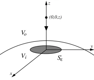
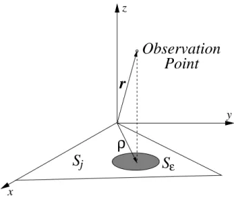
the overall integral does not evaluate to zero since the integrand tends to diverge when the observation point, r, approaches the source point, r0. Figure 2.1 shows that the observation point at (0, 0, z) approaches a smooth portion of the surface as z goes to zero. In the figure, Vi represents the interior of the closed object, so
ε ’
V
oV
i zS
(0,0,z) y xFigure 2.1: Observation point approaching a smooth portion of the surface from outside.
surface S0
ε is locally planar having its normal in the z direction and in the shape
of a circle with radius ².
Since the observation point becomes close to the source, Green’s function given in Equation (2.4) can be approximated as
g(r, r0) = eik|r−r
0|
4π|r − r0| ≈ 1
4π|r − r0|. (2.11)
In addition, source area is small enough that the current density can be assumed to be constant over the entire surface with a value of J(r0), where r0 = (0, 0, 0) is the point on the surface, which the observation point approaches in the limit. Then, the current density can be taken out of the integral and the expression for the scattered magnetic field from the infinitesimal surface becomes
Hscaε (0, 0, z) ≈ J(r0) × Z Sε dr0∇0 ³ 1 4π|r − r0| ´ . (2.12)
If the gradient expression is written explicitly as
∇0³ 1 |r − r0| ´ = R R3, (2.13) where R = r − r0 = ˆzz − ρ0, (2.14)
then Hscaε (0, 0, z) ≈ J(r0) 4π × Z Sε dr0R R3 = J(r0) 4π × ˆz Z 2π 0 dφ0 Z ε 0 dρ0 ρ 0z [(ρ0)2+ z2]3/2 −J(r0) 4π × ˆx Z 2π 0 dφ0 Z ε 0 dρ0 (ρ0)2cos φ0 [(ρ0)2+ z2]3/2 −J(r0) 4π × ˆy Z 2π 0 dφ0 Z ε 0 dρ0 (ρ0)2sin φ0 [(ρ0)2+ z2]3/2 = −J(r0) 2 × ˆz z [(ρ0)2+ z2]1/2 ¯ ¯ ¯ ¯ ε 0 = −J(r0) 2 × ˆz · z [ε2+ z2]1/2 − z |z| ¸ . (2.15)
As the observation point approaches the surface, z goes to zero and Hsca
ε (0, 0, z = 0) ≈
J(r0)
2 × ˆz. (2.16)
This result can be generalized as Hsca
ε→0(r0) =
J(r0)
2 × ˆn, (2.17)
where ˆn represents the normal of the surface in general.
When the observation point approaches a smooth portion of the surface, Equa-tion (2.17) indicates that the limit value of the magnetic field shown in EquaEqua-tion (2.10) has a magnitude equal to half of the current density and has a direction perpendicular to and in the same plane with the current flow. Consequently, if some current flow exists on a planar surface, the principle value of the magnetic field radiated by this current density is perpendicular to that plane, while the limit value forms the parallel component.
In general, the limit value depends on the solid angle of the surface at the ob-servation point, which is simply 2π for smooth surfaces. This dependence will
be shown explicitly in Chapter 4, but Equation (2.8) should be rewritten here as [14] Ωo 4πJ(r) − ˆn × Z S0(P V ) dr0J(r0) × ∇0g(r, r0) = ˆn × Hinc(r) (2.18) with Hscaε→0(r0) = Ωi 4πJ(r0) × ˆn, (2.19)
where Ωo represent the external and Ωi represents the internal solid angles of the
surface at the observation point, which may take values between 0 and 4π. It should be indicated that the Equation (2.18) relies on the assumption that the current density is continuous at the observation point.
2.2.2
Derivation by Using Interior Boundary Condition
If the observation point approaches the boundary from the interior of the closed surface, the boundary condition about the tangential component of the magnetic field should be written as
ˆ
n × Hinc(r) + ˆn × Hsca(r) = 0 (2.20)
if the surface is perfectly conducting. Using the expression for scattered magnetic field given in Equation (2.7),
ˆ
n × Hinc(r) + ˆn × Z
S0
dr0J(r0) × ∇0g(r, r0) = 0, (2.21) which seems to be different from (2.8). However, if the same procedure was applied to the radiation integral, then the limit value would be evaluated for smooth surfaces as Hsca ε→0(r0) = − J(r0) 2 × ˆn, (2.22) while it becomes Hsca ε→0(r0) = − Ωo 4πJ(r0) × ˆn (2.23)
in general. Using these limit expressions, Equation (2.21) changes into Equa-tion (2.18) again, although the derivaEqua-tion was based on a different form of the boundary condition.
2.3
Combined-Field Integral Equation
When the EFIE or the MFIE are used for the scattering problems of closed ob-jects, internal resonance problems arise at resonance frequencies. Both integral equations have nonzero null-space solutions, which adds extra current on the ob-ject in addition to the correct current distribution. The extra current from the solution of the EFIE does not radiate so that the far-field radiation can be calcu-lated correctly, even when the current is incorrect. However, null-space solution of the MFIE radiates and leads to incorrect calculation of far-field radiation [15].
To avoid the internal resonance problem, the combined-field integral equation (CFIE) can be used. This integral equation is simply the linear combination of the EFIE and the MFIE, and can be represented as
CFIE = αEFIE + (1 − α)MFIE, (2.24)
where α may take values between 0 and 1. Then, the CFIE can be written by combining the Equations (2.5) and (2.8) as
α · ˆ t · Z S0 dr0G(r, r0) · J(r0) ¸ +i k(1 − α) · J(r) − ˆn × Z S0 dr0J(r0) × ∇0g(r, r0) ¸ =i k · α ηˆt · E inc(r) + (1 − α)ˆn × Hinc(r) ¸ . (2.25)
It should be noted that the MFIE part is multiplied by the factor of i/k, in order to weight the equations equally before the linear combination.
Using the CFIE, two boundary conditions are applied at the same time and null-space solution of this equation is zero for all frequencies. In other words, the CFIE is free of internal resonance problem and it has unique solution for all frequencies. However, the CFIE has another advantage that makes it more preferable than the EFIE or the MFIE. As it will be shown later, matrix equations obtained by using the CFIE are generally better conditioned than the systems obtained by using the EFIE or the MFIE. This leads to relatively faster conver-gence of the iterative methods in the solution of the system, and gives superiority to the CFIE over the others [16]. Nevertheless, the MFIE and the CFIE cannot be used for the scattering problems of objects with open surfaces, and the EFIE becomes the only choice for those problems.
2.4
Method of Moments
Integral equations introduced in the previous sections can be represented in gen-eral as
L{f (x)} = g(x), (2.26)
where L is the linear operator of the equation, while f (x) is the unknown function that stands for the current distribution and g(x) is the excitation. To solve the problem, the unknown function can be expanded in a series of basis functions as
f (x) ≈
N
X
n=1
anbn(x), (2.27)
where an is the coefficient of the nth basis function. The basis functions should
be linearly independent and they have to be chosen appropriately, so that they can expand the current distribution. Then, defining the residual error as
R(x) =L ½XN n=1 anbn(x) ¾ − g(x) = ·XN n=1 anL{bn(x)} ¸ − g(x), (2.28)
the aim becomes to make this error arbitrarily small, in order the solve the problem not exactly, but with a small error. For this purpose, another set of functions called the testing functions, tm(x), can be used to weight both sides of
(2.28). Defining an inner product as ha(x), b(x)i =
Z
dxa(x) · b(x), (2.29)
Equation (2.28) can be tested for m = 1, ..., N as Z dxtm(x) · N X n=1 anL{bn(x)} = Z dxtm(x) · g(x). (2.30)
Finally, interchanging the order of summation and integration, the set of equa-tions becomes N X n=1 an Z dxtm(x) · L{bn(x)} = Z dxtm(x) · g(x) (2.31)
and a linear system can be formed as
N
X
n=1
anZmn= vm, (2.32)
where the matrix elements are Zmn =
Z
dxtm(x) · L{bn(x)} (2.33)
and the vector elements are vm =
Z
dxtm(x) · g(x). (2.34)
It is more evident in Equation (2.32) that N linearly independent equations are used to find the unknown coefficients of N basis function. In this equation, the matrix Z is usually called the impedance matrix, and the vector v is called the excitation vector. An element of the Z matrix at (m, n) is referred to as the interaction between the mth testing and nth basis functions.
The method described above is called as the method of moments (MOM) [1], which has been extensively used by many scientist in the solution of various types of scattering problems. By this method, an operator equation is reduced to a matrix equation. Therefore, it becomes possible to solve the linear equations involving continuous functions numerically with small errors.
2.4.1
Geometry Modelling and Meshing
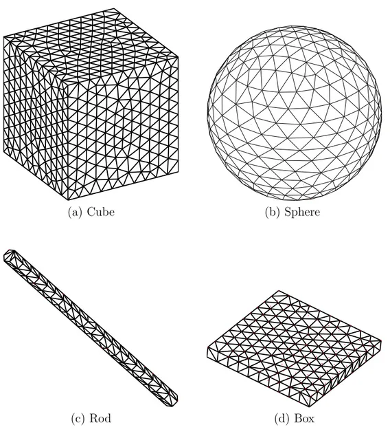
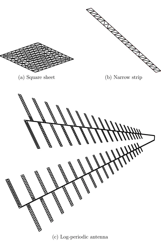
The application of the MOM requires the modelling of the problem geometries in the computer environment. Then, the surface models have to be meshed ac-cording to the type of the basis function to be used. Figures 2.2 and 2.3 show triangular meshing applied on various models of closed and open geometries. For high accuracy, the size of the triangles have to be small, which leads to large number of triangles or number of unknown coefficients, N. However, it becomes difficult to solve the linear system in (2.32) when N gets larger. The rule of thumb is to choose the average size of the mesh about 1/10 of the wavelength so that the MOM can be applied efficiently and with small error.
There are actually two error sources appearing at this stage. The first one is the approximation of the continuous current density with discrete functions. The second one is the modelling of the geometry with linear elements. The first error always exists, but it can be reduced by decreasing the element size. The second error, which also depends on the element size, exists only for the objects having curved surfaces, such as the sphere. In Figure 2.2(b), the smooth surface of the sphere is approximated by the combination of linear triangles.
Various types of basis functions can be defined on the triangular domains. For small error in the expansion of the current, high-order functions should be pre-ferred. In addition, the type of the linear operator also affects the choice [17], as
will be shown in the next subsection.
(a) Cube (b) Sphere
(c) Rod (d) Box
(a) Square sheet (b) Narrow strip
(c) Log-periodic antenna
2.4.2
Triangular Rooftop Basis Functions
Rao-Wilton-Glisson (RWG) functions are linearly varying vector functions de-fined on planar triangular domains [18]. Due to their useful properties, they have been widely used as basis and testing functions in MOM applications.
S
+nl
nO
n +S
n nr
r
r
− −Figure 2.4: RWG function defined on the triangular domains.
Figure 2.4 shows an RWG function defined on two triangles having a common edge of length ln. This RWG function associated with the nth edge is given as
bn(r) = ln 2A+ n (r − r+ n), r ∈ Sn+ ln 2A− n (r−n − r), r ∈ Sn− 0, otherwise , (2.35) where A+
n and A−n are the areas of the triangle surfaces Sn+ and Sn−, respectively.
Since the function is zero outside the two triangles and due to the symmetry of the expressions in the two triangular domains, an alternative definition can be attempted for the function on the ith triangle as
bik(r) = ± lik
2Ai
where δi(r) = 1, r ∈ Ai 0, otherwise (2.37)
is used to indicate that the value is zero outside the triangle. The alignment of the function on the triangle is represented by the index k = 1, 2, 3, which asso-ciates the function to one of the three edges of the triangle.
An important property of the RWG functions is that their divergence is finite everywhere. This comes from the fact that there is no discontinuity in the cur-rent flow that is crossing the boundaries of the triangles. Considering a single triangle, the current flow is purely tangential to two of the edges with no normal component. At the edge, to which the function is associated, the current flow has normal component; but it is continuous due to the corresponding current flow on the other triangle of the same function. It should be noted that, the value of the normal component becomes unity on the edge due to the normalization factors in (2.35). Therefore, the coefficient related to the nth basis function can
be interpreted as the value of the current flow across the nth edge.
In general, divergence of the RWG function can be written as
∇ · bn(r) = ln A+ n , rεS+ n − ln A− n , rεS− n 0, otherwise (2.38)
and the total charge associated with the function becomes A+ n ln A+ n − A− n ln A− n = 0. (2.39)
Equations (2.3) and (2.5) show that the implementation of the MOM with the EFIE requires the divergence operation on the current density. Therefore, it is appropriate to use the RWG functions to expand the current density, so that the
divergence operation is guaranteed to give bounded values. In addition, it will be shown that an efficient implementation of the MOM with the EFIE also requires the divergence of the testing functions. Therefore, it is also suitable to use the RWG functions as the testing functions. In general, the strategy of choosing the same type of basis and testing functions is called the Galerkin method. This method will be extensively used in the MOM and the fast-multipole-method (FMM) implementations presented in this thesis.
Chapter 3
MOM Implementations with the
EFIE
This chapter introduces the application of the MOM on the EFIE. The imple-mentation uses the RWG functions for both basis and testing functions. For efficiency, the impedance-matrix expression will be modified and divided into smaller integrals. In the evaluation of these integrals, it will be seen that the integrands tend to diverge as the observation point approaches the source point, due to the singularity of the Green’s function. To avoid numerical problems, singularity extraction method will be introduced to divide the problematic inner integral into analytic and numerical parts, each of which can be evaluated without any problem. Various methods will be explained to manage the numerical parts of the inner and outer integrals. Numerical results demonstrating the accuracy of the implementation will be presented at the end of Chapter 4.
3.1
Formulation
For conducting objects, the EFIE is given in Equation (2.5) as ˆ t · Z S0 dr0G(r, r0) · J(r0) = i kηt · Eˆ inc(r), (3.1)
where the observation point is on the surface. To apply the MOM, current density is expressed in terms of the basis functions as
J(r0) =
N
X
n=1
anbn(r0), (3.2)
where bn(r0) represents the nth basis function and an represents the coefficient
determining the weight of this basis function. Then, ˆ t · Z S0 dr0G(r, r0) · N X n=1 anbn(r0) = i kηˆt · E inc(r) (3.3)
and this equality can be tested as Z Sm drtm(r) · Z S0 dr0G(r, r0) · N X n=1 anbn(r0) = i kη Z Sm drtm(r) · Einc(r), (3.4)
where tm(r) represents the mth testing function. Rearranging the order of
sum-mation and integrals, the MOM system can be formed as
N X n=1 anZmnE = vmE, (3.5) where ZmnE = Z Sm drtm(r) · Z Sn dr0G(r, r0) · bn(r0) (3.6) and vE m = i kη Z Sm drtm(r) · Einc(r). (3.7)
Writing the dyadic Green’s function explicitly, the expression for the impedance-matrix element can be further divided as
ZmnE = Z Sm drtm(r) · Z Sn dr0 · I + ∇∇ k2 ¸ g(r, r0) · bn(r0) = Z Sm drtm(r) · Z Sn dr0g(r, r0)bn(r0) + Z Sm drtm(r) · Z Sn dr0∇∇ k2 g(r, r0) · bn(r0). (3.8)
If the basis and testing functions are chosen to be the RWG functions, the second part of the expression can be evaluated as
1 k2 Z Sm drtm(r) · ∇ ½ Z Sn dr0∇g(r, r0) · bn(r0) ¾ = 1 k2 Z Sm dr∇ · ½ tm(r) Z Sn dr0∇g(r, r0) · bn(r0) ¾ − 1 k2 Z Sm dr∇ · tm(r) Z Sn dr0∇g(r, r0) · bn(r0) = 1 k2 Z ∂Sm dl0u · tˆ m(r) Z Sn dr0∇g(r, r0) · bn(r0) − 1 k2 Z Sm dr∇ · tm(r) Z Sn dr0∇g(r, r0) · bn(r0), (3.9)
where ˆu represents the normal direction around the triangle pair of the function, as shown in Figure 3.1.
u
^
u
^
^
u
^
u
Figure 3.1: RWG function does not have current flow across its boundaries. Since the RWG function does not have normal current flow across its boundaries,
1 k2 Z ∂Sm dl0u · tˆ m(r) Z Sn dr0∇g(r, r0) · bn(r0) = 0 (3.10) and 1 k2 Z Sm drtm(r) · ∇ ½ Z Sn dr0∇g(r, r0) · bn(r0) ¾ = 1 k2 Z Sm dr∇ · tm(r) Z Sn dr0∇0g(r, r0) · b n(r0) (3.11) since ∇g(r, r0) = −∇0g(r, r0). (3.12)
A similar procedure can be applied on the inner integral, so that 1 k2 Z Sm drtm(r) · ∇ ½ Z Sn dr0∇g(r, r0) · bn(r0) ¾ = 1 k2 Z Sm dr∇ · tm(r) Z Sn dr0∇0· ½ bn(r0)g(r, r0) ¾ − 1 k2 Z Sm dr∇ · tm(r) Z Sn dr0g(r, r0)∇0· bn(r0) = 1 k2 Z Sm dr∇ · tm(r) Z ∂Sn dl0u ·ˆ ½ bn(r0)g(r, r0) ¾ − 1 k2 Z Sm dr∇ · tm(r) Z Sn dr0g(r, r0)∇0· bn(r0) = − 1 k2 Z Sm dr∇ · tm(r) Z Sn dr0g(r, r0)∇0 · bn(r0). (3.13)
Then, the impedance-matrix expression can be rewritten as ZmnE = Z Sm drtm(r) · Z Sn dr0g(r, r0)bn(r0) − 1 k2 Z Sm dr∇ · tm(r) Z Sn dr0g(r, r0)∇0 · bn(r0). (3.14)
Inserting the functions and their divergences explicitly by using Equations (2.36) and (2.38), ZE ik,jl = likljl 4AiAj Z Si dr(r − rik) · Z Sj dr0g(r, r0)(r0− rjl) − 1 k2 likljl AiAj Z Sm dr Z Sn dr0g(r, r0), (3.15)
where i and j indicate that the interaction is between ith and jth triangles, while
l and k represent the alignment of the basis and testing functions on these trian-gles. For an efficient implementation, it is essential to form the calculation loop over the triangles, instead of calculating the interactions between the unknowns. It will be shown that the basic integrals used in forming the impedance-matrix expression can be calculated without any alignment information. Then, con-structing the loop over the triangles makes it possible to avoid calculating the same integrals for nine times.
Before going on further, it should be noted that the divergence of a RWG func-tion is finite, so that no problem occurs in the second integral in (3.14). The advantage of using divergence-conforming functions in the EFIE-MOM appears more evidently at this stage. Since the divergence is also a constant, the integral reduces to a very simple form.
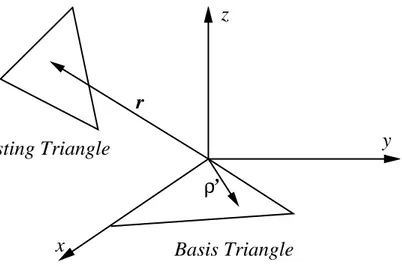
Basis Triangle
Testing Triangle
r
’
ρ
z
y
x
Figure 3.2: Location of the basis and testing triangles after the coordinate trans-formation.
Finally, a coordinate transformation can be applied, so that the basis triangle lies on the x-y plane with one of its edges on the x-axis, as shown in Figure 3.2. Such a transformation is essential in order to easily evaluate the analytic integrals appearing in the singularity extraction. The final expression for the interaction can be written as ZE ik,jl = likljl 4AiAj Z Si dr(r − rik) · Z Sj dr0(ρ0 − ρjl)e ikR 4πR − 1 k2 likljl AiAj Z Sm dr Z Sn dr0e ikR 4πR = likljl 4AiAj Z Sm dr(ρ − ρik) · Z Sn dr0ρ0eikR 4πR − likljl 4AiAj ρjl· Z Sm dr(ρ − ρik) Z Sn dr0e ikR 4πR − 1 k2 likljl AiAj Z Sm dr Z Sn dr0eikR 4πR, (3.16)
where
R = |r − ρ0| (3.17)
is the distance between the observation point and the source point.
3.2
Singularity Extraction
When the observation and source points approach each other, R goes to zero and the integrands of the inner integrals in Equation (3.16) diverges. For a numerical evaluation of these inner integrals, a suitable singularity extraction method has to be applied as Z Sj dr0eikR R = Z Sj dr0eikR− 1 R + Z Sj dr01 R (3.18) Z Sj dr0ρ0e ikR R = Z Sj dr0ρ0e ikR− 1 R + Z Sj dr0ρ0 R. (3.19)
It should be noted that
lim
R→0
eikR− 1
R = ik (3.20)
so that the first integrals on the right sides of Equations (3.18) and (3.19) can be evaluated numerically without any singularity problem, while other two integrals can be evaluated analytically [11, 12].
Evaluation of RSjdr01/R
Figure 3.3 shows the source triangle lying on the x-y plane with one of its edges on the x axis, and the projection of the observation point on the x-y plane, which may be located inside or outside the triangle. The integral can be divided into two parts as Z Sj dr01 R = Z Sj−Sε dr01 R + Z Sε dr0 1 R, (3.21)
where the region Sε represents the infinitesimal circular area centered at the
when the projection is outside, but it exists as a full circle when the projection is inside the triangle.
z y x
r
ρ
S
εS
jObservation
Point
Figure 3.3: Source triangle on the x-y plane and projection of the observation point.
By using the identity
∇0 S · µ R PPˆ ¶ = 1 R, (3.22) where P = |P | = |ρ − ρ0|, (3.23)
the integral can be evaluated as Z Sj dr01 R = limε→0 Z Sj−Sε dr0∇0 S· µ R PPˆ ¶ + lim ε→0 Z Sε dr01 R = lim ε→0 Z ∂(Sj−Sε) R PP · ˆˆ udl 0+ lim ε→0 Z α(ρ) 0 dφ Z ε 0 dP P (P2+ z2)1/2 = lim ε→0 Z ∂(Sj−Sε) R PP · ˆˆ udl 0+ α(ρ) lim ε→0 £ (ε2+ z2)1/2− |z|¤ = 3 X i=1 P0 i · ˆui Z ∂iSj R P2dl 0+ lim ε→0 Z Sε R PP · ˆˆ udl 0 + α(ρ) lim ε→0 £ (ε2+ z2)1/2− |z|¤ (3.24)
= 3 X i=1 P0 i · ˆui Z ∂iSj R P2dl 0 + α(ρ) lim ε→0 £ − (ε2+ z2)1/2+ (ε2+ z2)1/2− |z|¤ = 3 X i=1 P0 i · ˆui Z ∂iSj R P2dl 0− α(ρ)|z|. (3.25)
R
10 + +R
1 +R
1P
0 1 − − + − − 1 3 2u
u
u
^
^
^
x
z
y
z
|l |
1 −|l |
1 +Observation
Point
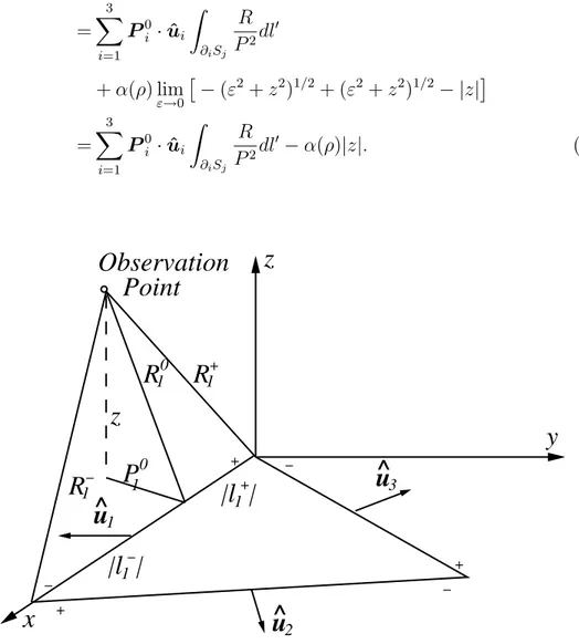
Figure 3.4: Geometric variables introduced to express the results of analytical integrals.
Finally, the integral can be written in terms of the geometric variables shown in Figure 3.4 as Z Sj dr0 1 R = −α(ρ)|z| + X i ˆ P0i · ˆui|z| · tan−1 |z|l + i P0 iRi+ − tan−1 |z|l − i P0 i R−i ¸ +X i ˆ P0 i · ˆui · P0 i ln µ R+i + l+i R−i + l−i ¶¸ , (3.26)
where the variables can be summarized as follows: • R+
i and R−i are the distances between the observation point and the end
of the edge are determined by the right-hand rule applied on the triangle in the z direction.
• R0
i is the distance between the observation point and the ith edge, which
can be written as
R0i = [z2+ (Pi0)2]1/2, (3.27) where P0
i is the distance between the projection of the observation point on
the x-y plane and the ith edge. In addition, ˆP0
i is the unit vector pointing
along the line between the projections of the observation point on the x-y plane and on the ith edge. The direction of this vector is towards the edge.
• l+i and li− have magnitudes equal to the “+” and “−” segments of the ith edge. These segments are formed by the projection of the observation
point on the edge. The signs of l+
i and l−i are determined by the relative
position of this projection compared to the “+” and “−” ends of the edge. In general, l± i |li±| = (ρei− ρ±) · (ρ−− ρ+) |(ρei− ρ±) · (ρ−− ρ+)|, (3.28) where ρei is the projection of the observation point on the ith edge, while
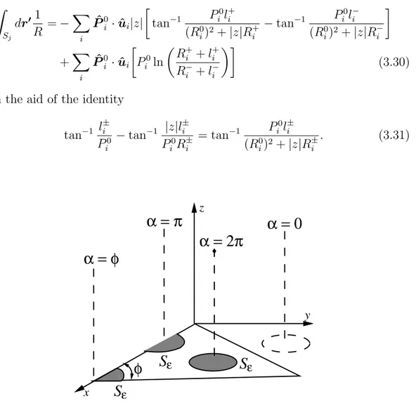
ρ+ and ρ− represent the “+” and “−” ends of the edge, respectively. In Equation (3.26), α represents the angular extent of ∂Sεlying within the
trian-gle, so that it becomes 2π when the projection of the observation point is inside the triangle and zero when it is outside. If the projection is on an edge or vertex, then α takes values between 0 and 2π. These cases are shown in Figure 3.5. In general, α(ρ) = 3 X i=1 ˆ P0 i · ˆui · tan−1 l+i P0 i − tan−1 l−i P0 i ¸ (3.29)
and Equation (3.26) can be rewritten as Z Sj dr01 R = − X i ˆ P0 i · ˆui|z| · tan−1 Pi0l+i (R0 i)2+ |z|R+i − tan−1 Pi0l−i (R0 i)2+ |z|R−i ¸ +X i ˆ P0 i · ˆui · P0 i ln µ R+ i + l+i R− i + l−i ¶¸ (3.30) with the aid of the identity
tan−1 l ± i P0 i − tan−1 |z|l ± i P0 i R±i = tan−1 P 0 i l±i (R0 i)2+ |z|R±i . (3.31) z y x
S
εS
εα = φ
α = π
α = 2π
α = 0
φ
S
εFigure 3.5: Different cases for the projection of the observation point.
Evaluation of RSjdr0ρ0/R This integral can be divided as
Z Sj dr0ρ0 R = Z Sj dr0ρ0− ρ R + ρ Z Sj dr01 R (3.32)
and it should be noted that the second integral has been evaluated. The first integral can further be divided into two integrals as
Z Sj dr0ρ0− ρ R = Z Sj−Sε dr0ρ0− ρ R + Z Sε dr0ρ0 − ρ R (3.33)
and the integrand can be written as ρ0− ρ R = −∇ 0 SR (3.34) so that Z Sj dr0ρ − ρ0 R = − limε→0 Z S−Sε dr0∇0 SR − limε→0 Z Sε dr0ρ − ρ0 R = − lim ε→0 Z ∂(S−Sε) Rˆudl0− lim ε→0 Z 2π 0 Z ε 0 P2 [P2+ z2]1/2dP dφ = − 3 X i=1 ˆ ui Z ∂iS Rdl0 = −1 2 3 X i=1 ˆ ui · (R0i)2lnR + i + li+ R− i + li− + l+i Ri+− li−R−i ¸ , (3.35)
where the final expression is reached by considering the geometric entities shown in Figure 3.4. Finally, Equations (3.35) and (3.30) can be combined as shown in (3.32) to complete the evaluation.
3.3
Evaluation of Impedance-Matrix Elements
For an efficient implementation, the expression in Equation (3.16) has to be divided into smaller integrals as
ZE ik,jl = likljl 4AiAj ½· − 4 k2 + xikxjl+ yikyjl ¸ Ie1+ Ie2+ Ie3 − xjlIe4− yjlIe5− xikIe6− yikIe7 ¾ , (3.36)
where the basic integrals can be listed as Ie1 = Z Sm dr Z Sn Ie1in, Ie2 = Z Sm dr, Z Sn xIe2in, Ie3 = Z Sm dr Z Sn yIe3in, Ie4 = Z Sm dr Z Sn xIe1in, Ie5 = Z Sm dr Z Sn yIe1in, Ie6 = Z Sm dr Z Sn Ie2in, Ie7 = Z Sm dr Z Sn Ie3in, (3.37)
and the inner integrals can be written as Ie1in= Z Sn dr0e ikR 4πR, Iin e2 = Z Sn dr0x0eikR 4πR, Ie3in= Z Sn dr0y0e ikR 4πR. (3.38)
Equation (3.36) indicates that the integrals can be evaluated without any align-ment information of the basis and testing functions. The evaluation of these seven basic integrals require the evaluation of three inner integrals. Then, their values can be used in forming the contributions to different locations in the impedance matrix. It should be noted that a triangle may belong up to three functions so that the contribution may be added up to nine different locations.
3.4
Numerical Evaluation of Integrals
The inner integrals in Equation (3.38) are divided into numerical and analytical parts as shown in Equation (3.18). The numerical parts of these integrals can be evaluated by using Gaussian quadrature rules. There are many of rules em-ploying different numbers of points on the triangle. In addition, the rules using different or same number of points can be combined to obtain new rules using larger number of points.
On the other hand, using a static rule in the implementation may result in in-correct integrations or inefficiencies. For an integration, if the number of points are less than the required, the final value may not converge to the exact value within a small error. In the other extreme, many integration points may be used, although few of them could already satisfy the convergence criteria. In addition, the distribution of the points may not be uniform and it would be better to take more samples, where the function changes rapidly, while taking less points for
smoother portions. As a result, instead of using high-ordered Gaussian quadra-ture rules, an adaptive algorithm can be used to control the integration error efficiently. Two different methods of adaptive integration will be presented here.
3.4.1
Adaptive Integration: Method 1
As shown in Figure 3.6, following steps are applied to evaluate the inner integrals on the basis triangle:
P P P1 3 2 Step 1 P 5 P4 P6 P3 P2 P1 Comparison Step 2 Step 3 Finish YES NO 1 2 3 Step 4 Step 4
Figure 3.6: Adaptive integration method 1.
1. On the triangle, three points are chosen, each of which is at the middle of an edge. As the Gaussian quadrature rule with three points states, the value of the integral is
I3 = · f (p1) + f (p2) + f (p3) ¸ Aj 3 , (3.39)
2. Three more points are taken on the medians of the triangle. These points are located at 1/3 of the median nearer to the vertices of the triangle. The value of the integral with six points becomes
I6 = · f (p1) + f (p2) + f (p3) + 2f (p4) + 2f (p5) + 2f (p6) ¸ Aj 9 . (3.40) 3. A comparison is performed on the 6-point versus 3-point integration values.
If the error, which can be defined as E3,6 =
|I6− I3| |I6|
, (3.41)
is less then the given error threshold, then the integration can be assumed to converge. Then, I6 can be returned as the value of the integral. If the error is large, more points should be sampled in order to achieve the desired convergence.
4. If the convergence is not satisfied, each of the three subtriangles can be considered as separate domains, on which the integrations are to converge individually, similar to the main triangle after first step. Three points are already evaluated on each of these subtriangles, and the process continues by taking three more samples to reach 6-point integrations.
5. The adaptive routine continues by comparing the results of the 3-point and 6-point integrations on subtriangles. Whenever convergence is reached in a subtriangle, one branch of the adaptive integration stops there, but the algorithm may go on in other subtriangles.
It should be noted that the algorithm completely stops only when the conver-gence is accomplished in all of the subtriangles of the basis triangle. In addition, the distribution of the points on the triangle is not uniform and more points are taken, where the function changes more rapidly. This is due to the fact that the algorithm continues to sample denser only on the non-converged regions.
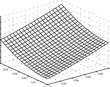
0 0.02 0.04 0.06 0.08 0.1 0 0.01 0.02 0.03 0.04 0.05 −0.3 −0.25 −0.2 −0.15 −0.1 −0.05 0 0.05 0.1
Figure 3.7: Function to be integrated on the triangular domain.
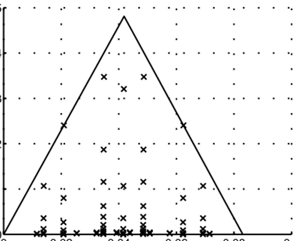
A disadvantage of this method appears when the aspect ratio of the integration domain gets larger. Figure 3.7 shows a function to be integrated on the triangu-lar domain with node coordinates (0, 0, 0), (0.083, 0, 0), and (0.042, 0.048, 0). As shown in Figure 3.8, the method continues to make divisions towards the edge on the x axis, but does not obtain a convergence. Actually, on the subtriangles near the edge, the new points are not located efficiently and they are very near to previous points. Therefore, the method tends to continue infinitely until an external stop. The second adaptive integration method avoids such divisions that create domains with high aspect ratios.
3.4.2
Adaptive Integration: Method 2
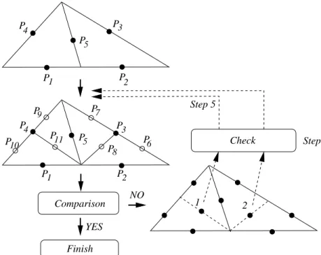
This method, described in Figure 3.9, consists of the following steps:
0 0.02 0.04 0.06 0.08 0.1 0 0.01 0.02 0.03 0.04 0.05 x y
Figure 3.8: Integration points taken by the first adaptive method to evaluate the integral of the function shown in Figure 3.7
value of the integral with five points can be written as I5 = · f (p1) + f (p2) + f (p3) + f (p4) + 2f (p5) ¸ Aj 6 . (3.42)
It should be indicated that two of the points are located on the longest edge of the triangle.
2. Six more points are taken on the triangle. To determine the location of these new points, the medians are drawn to the longest edge in each subtriangle. Then 9-point integration can be written as
I9 = · f (p1) + f (p2) + 2f (p5) + f (p6) + f (p7) + 2f (p8) + f (p9) + f (p10) + 2f (p11) ¸ Aj 12. (3.43)
It should be noted that the third and fourth points are not used in the 9-point integration.
3. A comparison on 5-point and 9-point integrations is made to determine the error as in the previous algorithm. If the convergence criterion is not satisfied, the process continues.