Implementation of a state-space Kalman filter on a digital signal processing microprocessor

(1)

î··^, M-j fjf". Д V S 3' j&j’l* Ê ; ,^ i ■ Ιζ^,Ιίϊίΐ^Ι Â îlf ■ГГІЙЕЙ. -O fê ' 0 п : А Ж

s у BMITTEp. T ö ■

·ΤΗΙ^" ·θ £PÄ^TMBp'r::

P

äü ; ·■;■' 'A k ù E t ü C r r n O M i O " ' •'‘■:D‘ ώ^·.··Γ:: • ^ ·,■;, 4^' -\ ■' :»·· ■ «'- '■* , -íy ,r-v': - ·-■ <t· ■** İÎp«>.J *·' W*' « ■ ■.W’'oil·'* í -iiıi-V ή· .--V^ ' — 1 • ^ “· I Ik .' · ! _ ."l \ ..I I ,r . ,Ml-k,m*l ,. , *1.. ^ <· , . i' I ■ .· '· ; . ■( ЧС »1,1, ^ 1 < [. , Д ,

(2)

IMPLEMENTATION OE A STATE-SPACE KALMAN

FILTER ON A DIGITAL SIGNAL PROCESSING

MICROPROCESSOR

A THESIS

SUBMITTED TO THE DEPARTMENT OF ELECTRICAL AND ELECTRONICS ENGINEERING

AND THE INSTITUTE OF ENGINEERING AND SCIENCES OF BILKENT UNIVERSITY

IN PARTIAL FULFILLMENT OF THE REQUIREMENTS FOR THE DEGREE OF

MASTER OF SCIENCE

tSiu...

-By

M. Khaledul Islam

August 1990

(3)

T к

v ¿~ u

•F5 Л /Г і

(4)

T o m y m o m w h o ta u g h t m e and A , В , C

(5)

I certify that I have read this thesis and thcit in my opinion it is full}' cnlequate., in scope and in quality, as a tliesis for the degree of Master of Science.

Asst. Prof. Dr. Gürhan Şaplakoğiu(Principal Advisor)

I certif}' that I have read this thesis and that in my opinion it is fully adecpiate, in scope and in quality, as a thesis foiv-fhe degree of Master of Science.

Asst Prof. Dr. Ta.yel E. Dabbous

I certify that I have read this thesis and that in rny opinion it is fully adequate, in scope and in quality, as a thesis for the degree of Master of Science.

rof. Dr. Hayrettin Köymen

Lib:

Approved for the Institute of Engineering and Sciences:

Prof. Dr. Mehmet>BAray

(6)

ABSTRACT

IMPLEMENTATION OF A STATE-SPACE KALM AN

FILTER ON A DIGITAL SIGNAL PROCESSING

MICROPROCESSOR

M. Khaledul Islam

M.S. in Electrical and Electronics Engineering

Supervisor: Asst. Prof. Dr. Gürhan Şaplakoğlu

August 1990

A general software written in assembly language for the real-time implementa tion of state-space Kalman filter on Texas Instruments TMS320C25 fixed-point digital signal processor is given. The software can accomodate dynamic system having up to 14 state variables. As a specific application, the Kalman filter is used to restore the sound of a flute embedded in white noise.

(7)

ÖZET

DURUM UZAYI KALMAN FİLTRESİNİN BİR SAYISAL

İŞARET İŞLETİCİSİNDE GERÇEKLEŞTİRİLMESİ

M. Khaledul İslam

Elektrik ve Elektronik Mühendisliği Bölümü Yüksek Lisans

Tez Yöneticisi; Yrd. Doç. Dr. Gürhan Şaplakoğiu

Ağustos 1990

Durum uzayı Kalman filtresinin gerçek zamanda, Texcis Instruments’in TMS320- C25 sabit noktalı sayısal mikroişlemcisi ile gerçekleştirilebilmesi için simgesel dilde yazılmış genel bir yazılım verilmiştir. Yazılım durum değişkeni sayısı en çok 14 olan dinamik sistemlere uygulanabilir. Kalman filtre, özel bir uygu lama olarak beyaz gürültüyle bozulmuş flüt sesinin yeniden elde edilmesi için kullanılmıştır.

(8)

ACKNOWLEDGMENT

I would like to express deep gratitude to my thesis supervisor Dr. Gürhan Şciplakoğlu for his invaluable guidance, stimulating inspirations and continuing help. Î am also indebted to him for introducing me to the fascinating world of real-time signal processing A special thank you goes to Mrs. Umay Şaplakoğlu who by playing flute played a vital role in our thesis progress. And last but not the least, I wish to acknowledge the assistance of Ergin Atalar who literally rescued me when I got lost in the schematic diagrams of SWDS board while making interfacing between 8088 and TMS320C25.

(9)

List of Figures

1.1 Kalman F ilte r ... 2

3.1 Compact Storage Scheme of Example 1 ... 14

3.2 Storage Scheme for LTA and M P Y pair o p tio n ... 24

3.3 Storage Scheme for M A C o p t io n ... 26

3.4 Storage Scheme for Sequential Processing, A = 8 . . . . 27

3.5 Storage Scheme for Batch Processing,

N = 8

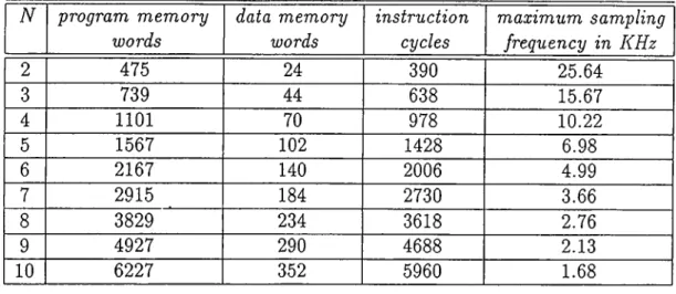
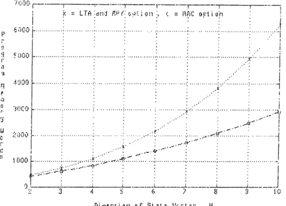
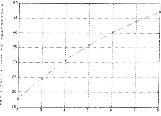
... 29

3.6 Program Memory Words Vs. Dimension of State Vector in Scalar O b serv atio n ... 33

3.7 Max. Sampling IVequency Vs. Dimension of State Vec tor in Scalar Observation... 33

3.8 Program Memory Words Vs. Dimension of Observation Vector in Vector O bservation ... 35

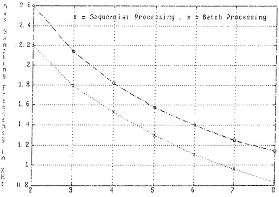
3.9 Max. Sampling Frequency Vs. Dimension of Observa tion Vector in Vector O bservation ... 35

3.10 Kalman Gain Computation Time Vs. Dimension of Ob servation V e c t o r ... 36

3.11 Comparison of LU and Choleski Decomposition 37 4.1 The Overall Setup for Kalman Filter Implementation . . 41

4.2 Flow-chart of 8088 and TM S Programs Running Simul taneously ... 42

(13)

LIST OF FIGURES

4.3 Filter Performance in Real-time Operation : the top most waveform is observation followed by filtered out put and actual n o t e ...

4.4 Filter Performance in Real-time Operation : the top most waveform is observation followed by filtered out put and actual n o t e ...

4.5 Performance of W N R and W F S methods (High SNR case:

Q

= 0.002,

R —

0.16, e = 1.02)

4.6 Performance of W N R and W F S methods (Low SNR case:

Q =

0.002,

R =

0.16,

e =

1.02)

4.7 Mesh Diagram of bandwidth vs. ki and «2, (for —0.4 < /Cl, «2 < 0.4 and

a =

0.809, /? = 0 . 5 8 8 ) ... 4.8 Effect of

Qy R

and e on P and

k.

a) Effect of SNR

for fixed

Qy Ry

e, b) Effect of increasing

Qy

c) Effect of increasing e 44 45 47 48 50 52

4.9 Effect of

R

on the Transient Response of the Filter Out

put 53

4.10 Effect of

Q

on the Transient Response of the Filter Out

put 54

4.11 Effect of e on the Tansient Response of the Filter Out

(14)

List of Tables

3.1 LTA and M P Y pair o p tio n ... 32

3.2 M A C o p tio n ... 32

3.3 Sequential Processing for

N = 8^ 2 < M < 8

... 34

3.4 Batch Processing for

N = 8, 2 < M < 8

... 34

4.1 Number of Harmonics of Flute N o t e s ... 39

D.l Addresses of Shared Memory as Seen by TMS and 8088 63

(15)

Chapter 1 INTRODUCTION

A brief introduction to the state-space Kalman filter and the digital signal pro cessors particularly Texas Instruments TMS320C25 is given in the first two sections of this chapter. Section three discusses the choice of fixed-point arith metic in real-time signal processing. The motivations behind choosing a digital signal processor fo r the implementation o f real-time fixed-point Kalman filter are described in section four.

1.1 The State-Space Kalman Filter

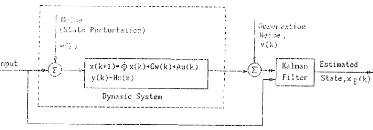
A discrete time Kalman filter is a recursive algorithm that calculates the linear, unbiased, minimum mean squared estimate of the state of a dynamic system from noise-corrupted observation data. The algorithm also allows random per turbations in the state evolution of the system. If the state perturbation noise and the measurement noise are uncorrelated and Gaussian, then the filter pro vides the best performance among all the estimators in mean squared sense. A very simple pictorial representation of the filter is given in Figure 1.1. Although the name filter sounds like a misnomer, it is the universally accepted term to describe the recursive algorithm that R. E. Kalman proposed back in 1960 [1]. The Kalman filter can be applied to any system that has a dynamic state-space representation. Apart from the state estimation of the system, it can also be used for system identification and deconvolution [2]. The wide spectrum of applications span as diverse fields as the space-craft orbit determination [3] and the demographic of cattle production [4]. Comprehensive treatment of the Kalman filter and its applications can be found in [5], [6], [7], [8] .

(16)

CHAPTER 1. INTRODUCTION J 07!) Ut j i .■> L P (5r't.ur 1:a t) c:■) ; ^

iy

_..J X(.k+-1)“ 0 X(k)+Gw(k)-^All(k) j ; I y(k)-H::(k) I , i---Dyna.Tiic Sy.stem

'.'o.'.-r.·! va :.i i.n' No: .ve , V (k) i Kalman F i l t e r Estimated State,X r (k)

Figure 1.1: Kalman Filter

1.2 T M S 320 Digital Signal Processor Family

Since Intel introduced the 2920 in 1979, the first microprocessor specifically tailored for digital signal processing applications, various VLSI digital signal processor chips have been launched by Texas Instruments, NEC, AT & T, Mo torola and many others [9]. Among these, Texas Instruments TMS320 family is one of the most widely used digital signal processors due to its relatively low cost, powerful instruction set, inherent flexibility and comprehensive hard ware support. The family consists of three generations of fixed and floating point digital signal processors. The second generation, which is considered in next chapters, comprises of five 16-bit microprocessors - namely TMS32020,

MS320C25, TMS320C25-50, TMS320E25 and TMS320C26. rn

1

Compared with conventional microprocessors, the most striking feature in TMS320 family is the use of parallelism and pipelining to enhance execution speed. It uses Harvard-type architecture which separates program and data memory spaces, eliminating the throughput bottleneck associated with the shared-bus structure of general-purpose microprocessors. This structure en ables data fetching concurrent with the fetching of next program instruction making the program execution faster. Another important difference is the fast fixed-point multiplication unit available in TMS320 family. As a matter of fact, the multiplier unit occupies most of the space(up to 40% in TMS32020) on the chip. Some of the key features of the TMS320C25, the most widely used member of the second generation which is considered in the subsequent chapters, can be summarized as [10] :

(17)

CHAPTER 1. INTRODUCTION

• 16 bit fixed-point operation with some provision for floating- point oper ation.

• 100 nanoseconds instruction cycle time which makes the microprocessor capable of executing 10 million instructions per second(MIPS).

• single cycle multiply/accumulate instruction with data move option thcit makes the digital filter realization very efficient.

• 544 words of on-chip RAM.

• 4K words of ROM that makes it a true single chip microprocessor. • total 64K words of program memory space and 64K words of data mem

ory space.

• 32 bit dedicated Central Logic Unit(CALU)

• 8 auxiliary registers with an Auxiliary Register Arithmetic Unit(ARAU) that operates in parallel with CALU

• sixteen input and sixteen output ports

1.3 W h y Fixed-Point Processor ?

All the members of the second generation TMS320 family perform 16-bit fixed- point arithmetic. The fixed-point arithmetic is based on the assumption that the location of the binary point is fixed. The Q notation is commonly used to specify the location of the binary point. A binary number in Qn format is defined as having n bits to the right of binary point. For example in sign- extension mode, the maximum and minimum numerical values represented by

Q15 format are hexadecimal 8000 and 7FFF or ecpivalently decimal -1 and

(1 — 2“ ^®) respectively. To get the Qn representation of a fractional number, the first step is to multiply it by 2" and round the result to an integer. The 2’s complement hexadecimal representation of the integer is the Qn equivalent of the corresponding fractional number.

Despite the fact that the fixed-point arithmetic has a limited dynamic range as compared to floating-point arithmetic, it does have some appreciable advan tages in real-time applications. First of all, the fixed-point digital signal pro cessors are much faster and cheaper than their floating-point counterparts. In floating-point arithmetic, errors due to arithmetic roundoff are introduced both

(18)

CHAPTER 1. INTRODUCTION

in addition and multiplication whereas in fixed-point arithmetic such errors o c cur only in multiplication. The major disadvantage of a fixed-point processor is the possibility of overflow. liowever, this problem can be overcome by using appropriate scaling. To be more specific, the program can be written in such a way that the occurance of overflow will depend solely on input samples. The necessary scaling can be determined by simulating the system on a floating point computer before real-time operation. Although the scaling may cause some loss in numerical accuracy, it is not usually significant. Another impor tant advantage of fixed-point arithmetic is the compatibility of the numerical representation used in the fixed-point digital signal processors and the analog interfacing devices. Most of the A /D and D /A converters available in the mar ket use either 2’s complement or offset binar}^ format to represent numerical values. This representation is very convenient when fixed-point arithmetic is used in Q15 format, because the input or output samples can be interpreted as

Q l5 representations of voltages normalized to the peak magnitude of convert

ers. The fact that the TMS320C5X, the 5th generation of the TMS320 family to be launched in late 1990, will be again a fixed-point processor reflect the preference of fixed-point arithmetic to floating-point arithmetic in real-time signal processing applications [11] .

1.4 Real-time Kalman Filter on a Fixed-point Digital

Signal Processor

Implementation of a Kalman filter involves heavy computational complexities. As far as conventional computers are concerned, the largest amount of program execution time is taken by multiplications. And to make things worse, the number of multiplications in Kalman filtering is proportional to the third power of the state size of the system [6] . Hence running a state-space Kalman filter on-line was not a realistic possibility until recently. Most of the real-time applications reported so far are applied to the systems that do not require fast execution times like navigation. The introduction of digital signal processors, which have very fast multiply/accumulate instructions, has opened a new era of real-time Kalman filter applications.

The TMS320 family is an ideal cost-elfective choice for implementing real time Kalman filters. Implementation of a simple two-state tracking Kalman filter on TMS32010, the first generation of TMS320 family, was reported [12]. Recently, implementation of a na,rrow-band Kalman filter on AT & T DSP32

(19)

CH APTE R !. INTRODUCTION

floating point processor has been published [13].

In this thesis, a general software written in TI assembly language version 5.0, is introduced to implement real-time Kalman filter on TMS320C25. The software consists of a collection of matrix manipulation macros, consequently can be modified to accommodate different Kalman filter algorithms. Efforts have been made to make an optimal trade-off between user-friendliness and execution speed of the software. As a matter of fact, our software is much more efficient in terms of speed as compared to [13] although DSP32 runs at a higher clock rate. Use of the software is thoroughly explained in chapter 3 along with illustrative examples. This chapter is preceded by chapter 2 which contains a review of Kalman filter algorithms and a discussion of the problems encountered in the implementation of the filter. As a specific application, real time implementation of state-space Kalman filter to recover the sound of a flute embedded in white noise is described in chapter 4. Based on simulation results, relationship between various filter parameters and their effects on filter gain and bandwidth are investigated.

(20)

Chapter 2 A R EVIEW OF THE K A LM A N FILTER

ALGORITHMS

In this chapter, different Kalman filter algorithms are reviewed. A variety of problems arise in real-time implementation of Kalman filter. Some o f the most likely problems are discussed in section two . Several criteria which can be used as tests fo r performance evaluation o f the filter are described in section three.

2.1 The Kalman Filter

Since R. E. Kalman published his landmark paper in 1960, it arouse great interest among researchers. The material is now well covered in literature [5],[6],[7],[8],[14],[15],[16]. A number of algorithms have been proposed as an alternative to the original Kalman filter algorithm. These algorithms make a trade-off between the numerical stability and the coiTiputational requirements. In the following sub-sections, some of the widely used algorithms are reviewed.

2.1.1 Notational Convention

The notational conventions used in the subsequent sections as well as in the following chapters are summarized below :

• vectors are lower-case letters with bars. • matrices are upper-case letters with hats. • [-]^ denotes transposition.

(21)

CHAPTER 2. A REVIEW OF KALMAN FILTER ALGORITHMS

• [·] ^ denotes inversion.

• x { j I k) is the estimate of x { j ) given the observation sequence

{y (n ) : n = 0 , 1 . . .

E { · } is the expectation operator.

2.1.2 The Algorithms

The Kalman filter requires that the relationship between the process to be estimated and the observation must be of the following state-space form :

x{k + 1) = ^{ k) x{ k) + Ğ{k)w(k),

y{k) = H{ k) x { k) + v{k),

(

2 .

1 )

(2.2)

where

x (k ) — N X 1 state vector at time ,

^ (k ) = N X N state-transition matrix at time , G(k) = N X L process noise matrix at time tk ,

w{k) = L X 1 process noise vector at time tk with known covariance matrix Q ( k ) ,

y{k) = M X 1 observation vector at time tk, H{ k ) = [ M X N ) observation matrix at time tk,

v{k) = M x l observation noise vector at time tk with known covariance matrix R(k).

Furthermore, the noise vectors are assumed to be white and uncorrelated with each other i. e. , E { v { i ) v ‘^ { j ) } =

Qi

if,

i = j

0 otherwise R i if,

i = j

0 otherwise |0) = 0 (2.3) (2.4) = 0 for V

i.

W ith these assumptions and notational conventions, some of the widely used Kalman filter algorithms are described in the subsequent subsections.

(22)

CHAPTER 2. A REVIEW OF KALM AN FILTER ALGORITHMS

Standard Kalman Filter

This is probably the most widely used form of the Kalman filter algorithm and is essentially the one that Kalman derived in 1960. It can be described in the prediction-correction form as :

• Step 1 : Initialization - A; = 0; Input ¿(0 | 0 ),P (0 | 0) • Step 2 : Prediction

-(2.5)

(2.6)

-b 1 1 A) (2.7)

1) -b R{k -b 1) (2.8) state prediction : x{ k 1 | A:) = ^ { k ) x { k | k)

covariance pi'ediction :

P { k -b 1 I A:) = ^ { k ) P { k 1 A:)I>^(A:) -J- Ğ(k)Q{k)Ğ'^{k) • Step 3 : Measurement - read y{k + 1)

• Step 4 : Innovation - innovation sequence :

u(^k T 1) = y(A; "T 1) — H(^k -t- l)x(A; -|- 1 | A;)

innovation covariance :

C{ k + 1) = H{ k + 1)P(A: -f 1 I A:)//^(A:

• Step 5 : Computation of Kalman gain

-Kalman gain : K { k + 1) = P(A: -f 1 | k) H^{ k + 1)C-^(A; -b 1) (2.9) • Step 6 : Correction -

state correction :

x(A: -b 1 I A: -b 1) = [ / - K { k -b 1)//(A^ + l)]â;(A· -b 1 | A:)+

K { k + l ) y{ k + l) (2.10)

covariance correction :

P{ k -b 1 I A^ + 1) = [ / - K { k + l ) H ( k + l ) ] P{ k -b 1 I A) (2.11)

• Step 7 ; Continuation - A = A -b 1, go to Step 2

A major drawback of this algorithm is the fact that the covariance matrix

P { k -b 1 I A -b 1) is prone to numerical roundoff errors and may loose positive

definitiveness resulting in serious errors. Even the symmetry of P can be lost in a few iterations as a direct result of fixed-length numerical computations [18].

(23)

CHAPTER 2. A REVIEW OF KALMAN FILTER ALGORITHMS

Stabilized Kalman Filter

This method is superior to the standard Kalman filter since it is less sensitive to numerical roundoff. As expected, the price paid for it is more computational burden. The steps of the algorithm are the same as the standard one except the covariance correction in step 6. In this case, the filtered estimate of the error covariance matrix is computed as,

P(A: + 1 I A: + 1) = K { k + l ) R { k + l ) K { k + l f +

[I - K { k + l ) H { k + l ) ] P{ k + 1 I ^-)[/ - K { k + l ) H { k + l ) f (

2

.

12

)

This expression of P in the form of sum of two symmetric matrices is called “Joseph form” . Numerical computations based on this form are better condi tioned and symmetry as well as positive definitiveness of matrix P are preserved [17].

Sequential Kalman Filter

The sequential algorithm refers to the technique of processing the measure ment vector y{k) one component at a time as opposed to the batch processing where all the elements of the observation vector are treated at the same time. The beauty of this algorithm is that the direct computation of inverse of the innovation covariance matrix C is avoided. This results in appreciable amount of computational savings. The sequential algorithm can be applied when the covariance matrix of observation noise, R( k) is diagonal. However, this is not a big constraint, since the observation y(k) can always be transformed to an uncorrelated process say y(k) with a diagonal covariance matrix R{k) by a nonsingular transformation D{k). In doing so, the observation equation ,

becomes.

y{k) = Hx { k ) + v{k)

y{k) = Hx { k ) -f v{k)

(2.13)

(2.14) where, y{k) = D{ k) y{ k) , H{ k) = D{ k ) H( k ) , v{k) = D( k) v{ k) such that

S ( j ) } = D( k) R( k) D^{ k) . Details of the algorithm can be found in

(24)

CHAPTER 2. A REVIEW OF KALM AN FILTER ALGORITHMS 10

Square Root Algorithm

As compared to the previous algorithms, the square root filter is better from an accuracy point of view. The reason is that square-rooting a small number- yields a large number and vice versa, thus computations are carried out more precisely. The core of this algorithm is the Choleski decomposition which decomposes a non-negative definite symmetric matrix A into the product of a lower triangular matrix A^^ and its transpose such that.

A = A^(A^)c\T (2.15)

If all the components of the measurement vector are treated at the same time as in the standard and the stabilized filter, the inversion of a lower triangular matrix is needed. On the other hand, the sequential processing can be incorpo rated into the square root algorithm thus making a good compromise between the computational requirements and the numerical accuracy[14].

A comparison between these algorithms in terms of memory reciuirements and execution speed can be found in [18]. However, the comparison is based on the assumption that the multiplication takes thrice as much time as addition which is the case with general-purpose computers.

2.2 Practical problems in real-time Kalman filtering

Some of the usual problems encountered in real-time Kalman filtering are de scribed in the following subsections.

2.2.1 Roundoff Errors

As with all digital hardware of finite word-length, fixed-point implementation of Kalman filter is not immune from unavoidable roundoff errors. Due to recursive nature of the algorithm, these errors may be quite significant. One of its worst consequences reported by many researchers, is that the covariance matrix P may become negative definite due to the accumulation of roundoff errors [16]. This leads to instability of the filter. One solution is to add some process noise i. e. to perturb the evolution of the state by a random disturbance even if the system is known to be deterministic. In doing so, the positive definite Q matrix prevents the error covariance matrix P from going

(25)

CHAPTER 2. A REVIEW OE KALM AN FILTER ALGORITHMS 11

negative as evidenced from the prediction step of the algorithm. This imposed uncertainty leads to a degree of suboptimality, but it is better than having the filter diverge. Another solution is to symmetrize

P(k

+

1

|

k)

and

F(k-j-l |

A;+l)

matrices at each iteration step. Since covariance matrix must be symmetric, any form of asymmetry can be attributed to roundoff errors. The symmetry problem is automatically solved if, in implementation symmetry of covariance matrix is assumed and only the lower (or the upper) triangular part is used and updated in all operations. Another way is the square root algorithm which propagates the square root of

P

rather than the

P

itself. Various other methods have been proposed to encounter this problem [19], [20].

2.2.2 M odel Mismatch

Inaccuracy in system-modeling can severely deteriorate the filter performance. The errors associated with model mismatch can be minimized to certain extent by adding fictitious process noise. A more effective way to accomplish this is to use fading memory filter which takes into account the gradual change in system parameters by exponentially diminishing the effects of older data on recent cal- cula.tions [17]. Basically this means that as one moves along time, the strength of corrupting noises in prior iterations are artificia.lly increased before their influence is brought into current estimation of the states. For example, if the conventional Kalman filter provides state estimates at time ti based on obser vation noise sequence R{ti), R{ t2) ■ · ■ R{ti) then the fading memory filter would

do so using the exponentially decaying sequence e'^^R(ti), e‘'^R{t2) ■ ■ ■ e^'R{ti).

The term e°' is called the “ forgetting factor ” since it determines how heavily the recent data are overweighed. It can be shown that the fading memory has the same steps as conventional Kalman filter with a minor change in the prediction of error covariance matrix

P{k A I \

k)

which in this case is given by,

P{ k + l \ k ) = ^ k ) P { k I d- G{k)Q{k)G'^'{k).'^T(

(2J6)

For completeness, the derivation of the discrete time fading memory is given in Appendix A following [21].

2.2.3 Observability Problems

This problem arises when the system is not observable i. e. one or more of the state variables(or their linear combinations) are hidden from the view of

(26)

CHAPTER 2. A REVIEW OF KALMAN FILTER ALGORITHMS 12

the observer [16]. As a result, if the unobserved states are unstable, the corre sponding estimations will be unstable. The occurance of such a problem can be evidenced by the unbounded growing of one or more diagonal entries of error covariance matrix.

2.3 Tuning of Kalman Filter

The estimates of states of a system as provided by Kalman filter is optimal only if the filter is properly “tuned” . A couple of parameters can be checked to ensure that the filter is operating properly. A necessary and sufficient condition for the Kalman filter to be working properly is that the innovation sequence must be zero-mean and white [8]. This can be easily checked in practice. The square roots of the diagonal entries of the covariance matrix P represent the root-mean-square(RMS) error associated with the states [2]. If the filter is properly tuned, the diagonals should reach steady-state values irrespective of initial assumption P (0 | 0). This arises from the fact that as long as the filter is stable and the state-space model is completely controllable and observable, then P attains a steady state value [8]. It should be noted that initial guesses on the state vector a-(0 | 0) and covariance matrix P(0 | 0) are not important in tuning the filter since their effects are reduced as more observation data are processed.

(27)

Chapter 3 A GENERAL SOFTWARE FOR

FIXED-POINT IMPLEMENTATION OF

REAL-TIME KALM AN FILTER

In this chapter, a general software written in TI assembly language fo r the implementation o f fixed-point Kalman filter on TMS320C25 digital signal pro cessor is introduced. Use o f macro library fo r various implementations o f the filter algorithms are described and illustrated with examples. A comparison

between these approaches is discussed in the last section.

3.1 A Software for Kalman Filter : A n Introduction

A very general user-friendly software in the form of macros is written in Texas Instruments(TI) assembly language version 5.0 for TMS320C25 digital signal processor in order to implement real-time fixed-point Kalman filter having as many as 14 states. Any of the filter algorithms discussed in chapter two can be implemented using these macros. As a matter fact, the extensive macro library provides the user with a wide choice implementations. To incorporate the macros in the main program, the user does not have to be an expert of TI assembly language. As illustrated with examples in the next sections, only a little knowledge of TMS assembler directives and its memory configuration is enough to efficiently use the macros in filter algorithm. Since one of the prime concerns in the implementation of real-time Kalman filter is execution speed, macros are preferred to subroutines at the expense of considerable demand on program memory. The macros are written in such a way that they fully exploit the unique architecture of the TMS microprocessor. Some of the steps in the

(28)

CHAPTER 3. A GENERAL SOFTWARE FOR KALMAN FILTER 14

filter realization are rearranged to make them more suitable to TMS structure. The macros are written with the assumption that all numerical computations are carried out using fixed-point Q15 format.

3.2 The Storage Strategy Used in the Software

A general storage strategy is used for storing scalars, vectors, matrices in all the macros. It is assumed that maximum allowable size of a matrix is 14 x 14. For matrices, the entries of a row are stored in consecutive places whereas those of a column are stored hexadecimal 10 (decimal 16) places apart in memory. The only exception to this rule is the storage of diagonal matrices. In this case, the diagonal entries are stored in successive memory locations. When we say that a matrix A is stored at “Loc_of_A” in data memory, we simply mean that A (l, 1) is stored right at “Loc_of_A” and the remaining entries are stored relative to this location. For example, storing A at hexadecimal 211 (denoted as 211h) means that A ( l , l ) is stored at 211h, A (l,2 ) at 212h, A ( 2 ,1) at 221h and so on. The same storage strategy holds for vectors i. e. elements of a row vector are stored in consecutive places whereas those of a column vector are placed hexadecimal 10 places apart. This storage strategy facilitates efficient use of memory and at the same time enables the user to visualize everything in terms of the usual indexing used in vectors and matrices. Example 1 illustrates how this can be used to store different matrices and vectors in compact form in the memory.

E x a m p le 1

Let us suppose that A is a 6 x 8 matrix, .6 is a 7 x 7 matrix, T) is a 8 x 8 dicigonal matrix, e is a 1 x 8 row vector and / is a 8 x 1 column vector. Now if the available memory starts from 300h, then all these parameters can be stored in a compact form as illustrated by Figure 3.1.

(300h)-A(l,l) . (310h)-A(2,l) . . . (307h)-A(l,8) . . (317h)-A(2,0‘; (350h)-A(6,l) .. (357h)-A(6,fl) (360h)-D(l,l) .. . (367h)-D(8,8) (370h)-e(l) ..., . (377h)-e(7) (308h)-B(l,l) (318h)-B(2,l) (378h)-e(8) (30Eh)-B(l,7) (31Eh)-B(2,7) (368h)-B(7,l) ... (36Eh)-B(7,7) unused 6 locations (30Fh)-f(l) (31Fh)-f(2) (36Fh)-f(7) (37Fh)-f(8) Figure 3.1: C o m p a c t S tora g e S ch em e o f E x a m p le 1

(29)

3.3 The Macro Library

The extensive macro library provides a variety of implementation of the Kalman filter. Appendix F contains all the macro codes which are written with exten sive comments.

3.3.1 General Matrix Macros

A brief summary of the general macros is given below :

1. M ake necessary Initialization • macro ; Makelnit

• operation : Make general initializations that are used by all macros • description : make necessary initialization for fixed-point Q15-based

numerical computation 2. Scalar A ddition or Subtraction

• macro : ScalAorS Location, OPTION • operation :

(a) [ACCH] + [Location] — ^ [ACCH], if OPTION = 0 (b) [ACCH] - [Location] [ACCH], if OPTION = 1

• description : add (or subtract) a scalar value stored at “Location” to (or from) high accumulator(ACCH)

3. V ector A ddition or Subtraction

• macro ; VectAorS M, Loc_of_a, Loc-oLb, OPTION • operation ;

(a) a + b — *· a, if OPTION = 0 (b) a - b — > d, if OPTION = 1

• description : add (or subtract) an M X 1 column vector b stored at “Loc_of-b” in data memory to (or from) another M x 1 column vector d stored at “Location_of_a” in data memory and store the resulting vector in a ’s place

(30)

• macro : VectMorD M, Loc_of_a, L oc.oL c, OPTION • operation ;

(a) a x [ACCH] ^ c, if OPTION = 0 (b) [ACCH] ^ c, if OPTION = 1

• description : multiply (or divide) an M x 1 column vector d stored at “Loc_of_a” in data memory by a scalar stored in upper-half of accumulator and store the resulting vector c at “Loc_of_c” in data memory

5. V ector V ector Multiplication

• macro : VecVecMl M, Loc_of_a, Loc_of_b, Loc.oLC, OPTION • operation :

(a) d(row vector in data memory) x¿(colum n vector in data mem ory) — > [ACCH] , if OPTION = 0

(b) d(coIumn vector in data memory) x [¿(column vector in data memory)]^ — > C(only the lower-half) , if OPTION = 1

(c) d(row vector in program memory) x ¿(column vector in data memory) ^ [ACCH], if OPTION = 2

• description : find inner-product (or outer-product) of two vectors a and b stored at “Loc-oLa” and “Loc_of_b” respectively and store the inner-product in high accumulator (or the lower-half of the outer- product at “Loc-oLC” in data memory)

6. M atrix A ddition or Subtraction

• macro : Mat_AorS M, Loc_of_A, Loc_oLB, OPTION • operation :

(a) A(lower-triangular matrix)+B(lower-triangular matrix) — ^ A, if OPTION = 0

(b) A(lower-triangular matrix)—J5(lower-tricmgular matrix) ^ A, if OPTION = 1

(c) A(lower-triangular matrix)-[-¿(diagonal matrix) — »■ A, if OPTION = 2

description : add (or subtract) an M x M lower-triangular matrix or diagonal matrix B located at “ Loc_oLB” in data memory to (or from) a,n M X M lower-triangular matrix A located at “Loc_oLA” in data memory and store the resulting lower-triangular matrix in A ’s place

(31)

CHAPTER 3. A GENERAL SOFTWARE FOR KALM AN FILTER 17

7. M atrix M a trix Multiplication between program memory and data mem ory

• macro ; MtMtMlpd M, N, P, L oc.oL A , Loc_oLB, Loc_of_C, O P T IO N -l, 0P T I0N _2

• operation :

(a) A (in program memory) xJ5(in data memory) — > C, if OPTION-1 = 0 and 0 P T I0 N .2 = 0

(b) [A(in program memory) x 5 ( i n data memory)]^ — >· C, if O P T IO N .l = 1 and OPTION_2 = 0

(c) A (in program memory) x.6(in data memory) — >■ ¿/(only the lower-half), if OPTION-1 = x(don’t care) and OPTION-2 = 1 • description : multiply an M x N matrix A stored at “L oc-oL A ” in program memory by an A ”x T matrix B stored at “ L oc-oL B ” in data memory and store the resulting matrix or its transi>ose or the only the lower-half of resulting matrix (if it is known to be symmetric beforehand) at “L oc-of-C ” in data memory

8. M atrix M a trix Multiplication between data memory and data memorIT • macro : MtMtMldd M, N, S, T, Loc-oLA, L oc-oLB , Loc-oLC,

OPTION -1, 0 P T I0 N .2 • operation :

(a) A (in data memory) x ¿ ( i n data memory) if OPTION-1 = 0 and OPTION-2 = 0 (b) [A(in data memory) x ^ (in data memory)]^

if OPTION-1 = 1 and OPTION-2 = 0

(c) A (in data memory) x ¿ ( i n data memory) — ^ ¿ (o n ly the lower-half), if OPTION-1 = 0 and OPTION-2 = 1

(d) A ^(in data memory) x ¿ ( i n data m em ory)— >■ C, if OPTION-1 = 1 and 0P T I0 N _2 = 1

• description ; multiply an M x N matrix A (or its transpose) stored at “L oc-of-A ” in data memory by an 5 x T matrix ¿ stored at “L oc-of-B ” in delta memory and store the resulting matrix or its transpose or the only the lower-half of resulting matrix (if it is known to be symmetric beforehand) at “Loc-of-C ” in data memory. Note that for the first three options, N = S, else M = S

(32)

• macro : FilLMat M, Loc_of_A

• operation : A(lower-triangular matrix) — > A(symmetric matrix) • description : fill the upper-half of a M x M lower-triangular matrix

A stored at “Loc_of_A” in data memory with its lower-half and

thereby symmetrize the matrix 10. M atrix C op y in g

• macro M at-Copy M, N, SOURCE, BEST

• operation : A(at SOURCE in data memory) — > A(at BEST in data memory)

• description : copy a,n M x N matrix A stored at “SOURCE” in data memory to “BEST” in data memory

11. M o v e from Program memory to D ata memory

• macro ; Move_P.B M, N, SOURCE-P, BEST-B

• operation : A(at SOURCE.P in program memory) — )· A(at BEST-B in data memory )

• description : move &n M x N matrix A stored at “SOURCE-P” in program memory to “B E S T -B ” in data memory

12. Q15 D ivision

• macro : Q15-Biv

• operation : [ACCH] ^ [065h] — ^ [ACCL]

• description : divide a Q15 number stored in high accumulator(ACCH) by another Q15 number stored at 065h of data memory and store the result in low accumulator(ACCL)

13. LU -Factorization of a symmetric matrix • macro : LU-Fact M, L oc-oL A , Loc-oLC

• operation ; /l(lower-traingular matrix) — > C — L x U = A

• description : From the knowledge of lower-half of a symmetric ma trix A stored at “L oc-oL A ” in data memory, perform LU decom position such that C = L X U = A, and store it in compact form at “L oc-of-C ” in data memory, where L is the lower-triangular half and U is the upper-triangular half of C. The diagonal entries in

C correspond to those of A, whereas diagonals of U are not stored

(33)

14. solve a system of equation by F o rW a rd substitution

• macro : For_VVard M, N, Loc-oLL, Loc_of_B, Loc_of_Y • operation : solve Y from L Y —

• description : using forward substitution, solve Y from L Y = ,

where Z is an M x M lower-triangular matrix stored at “Loc_of_L” in data memory and В is &n N x M matrix stored at “Loc_of_B” in data memory. Y is stored at “Loc_of_Y” in data memory

15. solve a system of equation by B a ck W a rd substitution • macro : Bck_Ward M, N, Loc_of_U, L oc-oL Y • operation : solve X from U X = Y

• description : using backward substitution, solve X from U X = Y where is an M x M upper-triangular matrix with diagonals as I ’s stored at “Loc_of_U” in data memory and Y is M x N matrix

stored at “ L oc.oL Y ” in data memory, and store X in Y ’s place 16. find S q u a re -R o o t of a Q15 number

• macro : Sqr_Root

• operation : ^[ACCH] ^ [ACCL]

• description : find the square-root of a Q15 number stored in high accumulator(ACCH) by Newton-Raphson method and store it in low accumulator(ACCL)

17. C h o le s k i factorization of a symmetric matrix • macro : Choleski M, L oc.oLA

• operation : A(lower-traingular matrix) — > C = A ‘^{A^)'^

• description : From the knowledge of lower-half of a .symmetric uia-

trix A stored at “Loc_of_A” in data memory, perform Gholeski- decomposition such that A = A ‘^(A‘^)'^ and store the lower-triangular matrix /F in A ’s place

18. perform Sequential Processing

• macro : ,Seq_Proc M, N, Loc_of_H, Loc_of_P, Loc-oLR , Loc_of_y, Loc_of_x, Loc-oLk, tem p.l, temp_2

(34)

description : for vector observation case, find filtered estimates of the state vector x{ k + 1 | A: + 1) and the error covariance matrix P(A: + l|A: + l ) b y sequential processing as discussed in last chap ter, where MxA^ matrix H, N x N m&tvix P, M x M diagonal matrix

R, M X 1 column vector y and x 1 column vector x are stored

at “Loc_of.H” , “L oc.oL P ” , “ L oc.oL R ” , “ Loc_of_y” and “Loc.oLx” in data memory respectively. The intermediate result k is stored at “Loc_of_k” whereas “tem p_l” and “ temp.2” are N x N and A'' x 1 storage locations used for temporary storage.

3.3.2 Some Special Macros

To get rid of unnecessary computations like multiplication with ones and zeros or addition with zeros, some special macros are written when state transition matrix $ have the following block diagonal structure :

$ = ■ 1 0 ₁₁ 1 0 0 1 1 * 2 1 1 1 : 1 0 . 0 1 1 0 1 $.· . = Pi (3.1)

and observation vector h is of the form

h = hi I }l2 hi > 1 0 (3.2)

where 1 < i , j < 4. In these macros, the observation vector Ji does not have to be stored . Another important feature is that state vector x is stored as a row vector . The upper-half of error covariance matrix P is never calculated and in the computations, P is assumed to be symmetric. This results in considerable scivings when Kalman filter having the above mentioned state-space structure is implemented using these special macros.

1. Find P R E D icte d ESTimates of state vector and error covariance matrix • macro : PRED-EST N, Loc_of_Phi, Loc.oLP, Loc_of-x, Loc-oLQ • operation : x and -h Q — >

P

(35)

• description ; find predicted estimates of the state vector x(k + 1 \ k)

and the error covariance matrix F { k+ 1 | k) where TV xfV block diag

onal matrix l>, TV X TV lower-triangular (symmetric) matrix T°, 1 x TV vector X and TV x TV diagonal matrix Q are stored at “Loc_of_Phi” , “Loc_of_P” , “Loc_of-x” and “Loc_of_Q” in data memory respec tively. The macro uses three other macros namely MAT221, MAT222 and PH L X for operations on 2 x 2 block matrices.The operations performed by these three macros are :

- MAT221 : A5(lower-triangular)A^ + ¿^(diagonal) - MAT222 : ABC'^ — ^ C

- PHI_X :

B

X

2. Find FILTered ESTimates of state vector and error covariance matrix • macro : FILT-EST N, Loc.oLP, temp_l, Loc_of_r, Loc_of-k, Loc.oLx,

Loc_of_y

• operation : Ph^l\hPh^ -f i2] — > k, P — Ph^k^ — > P and X — k[hx — y] — > x

• description : find filtered estimates of state vector

and error covariance matrix P { k + 1 | ¿ - f l ) whei’e TV x TV lower- triangular matrix P, observation variance T?, 1 x TV vector x and observation y are stored at “L oc-of-P ” , “Loc_of_r” , “Loc_of_x” and “Loc_of_y” in data memory respectively. It should be noted that this is a special macro which serves some other specific purposes. To communicate with the outside world, it resets external flag(XF) to get data. The new data is written into “Loc_of_y” by the exter nal processor whereas previously processed data which is the sum of every other entries of filtered state vector is written into next location. At the end of the macro, the external flag is set. As far as I/O operations are concerned, the macro converts offset binary(OB) format into 2’s complement format and vice versa.

3.4 Building up the Kalman Filter Algorithms

The wide choice of macros provides a variety of standard and user-defined implementations of the Kalman filter. While using the macros in the filter algorithm, the architecture of the TMS processor has to be exploited to get the best throughput. For example, the multiplication of two operands (vectors

(36)

or matrices) can be very efficiently performed at minimum cost of program memory by putting one operand in program memory and the other in data memory. The TMS320C25 digital signal processor has 544 words of on-chip data RAM of which 256 words can be configured either as program memory or data memory by a software command (C N FP/C N FD instruction). Apart from this, all the system boards that are developed around the TMS320C25 chip have no-wait-state external RAM which can be as large as 123K. As far as execution speed is concerned, the most efficient implementation requires that both the data and the program space should reside in on-chip RAM . How ever, because of macro-based straight-line code implementation, the program occupies considerable space. To make an optimal trade-off between speed and memory space, the macros are written mostly from the first four classes of in struction set for which running the program from no-wait-state external RAM with data in on-chip R AM is as fast as executing from on-chip RAM. According to the number of cycles required for execution, all the instructions are grouped into fifteen classes. When both the program and the data are in on-chip RAM , the first four classes take one instruction cycle. On the other hand, for ex ternal program R AM and on-chip data RAM each instruction takes (p -|- 1) cycles where p is the wait state of external program memory. Hence it is rec ommended to store the data and the intermediate results in on-chip data RAM and run the program from no-wait-state external program RAM for which p =0.

One of the most-likely problems encountered in implementation of the Kalman filter is the divergence of error covariance matrix P as discussed in chapter two. This problem is automatically solved as the macros concerning the predicted and the filtered estimates of P calculate only its lower-half and then fills the upper-half making sure that the symmetry is preserved. In the correction part of error covariance matrix P, the filter step terms are rearranged to make it more suitable for TMS structure. Since the error covariance P{ k -f 1 | -f 1) given by.

P { k + 1 \ k + 1) = [I - K { k -f l ) H ] P ( k + l \ k ) (3.3)

is symmetric, it can be written as,

P{ k + l \ k + l) = P'^{k + 1 I A; + 1)

=

[P{k

+ 1 I ^) -

K(k + l)HP(k

+ 1 I

k)f

= P{k + 1\ k)

- -h 1 I

k)H^K'^{k

-f 1) (3.4)

The term P (^ -l-l | k) H^ needs to be calculated for the computation of Kalman gain in the preceding step. Hence, it can be stored in a temporary storage location and readily used in error covariance correction. For TMS320C25, this

(37)

form of realization o f

P{k+1

| ¿ + 1 ) is computationally faster than its standard form.

The macros can be used to define a new user-defined macro. While doing so, two important points should be taken into account - the auxiliary register ARO should not be changed and the data memory locations 65-68h of on-chip block BO should not be used.

The implementation of the Kalman filter using the macro library is dis cussed in the following subsections with examples.

3.4.1 Scalar Observation

For scalar observation, two different approaches are considered. The first ap proach is called “LTA and M P Y pair option” because of frequent use of these two instructions in multiplication. In this case , the data and the intermediate results are stored in data memory. In the second implementation, they reside either in program memory or data memory to exploit the fast M AC(M ultiply and Accum ulate) instruction and hence is called “MAC option” .

LTA and M P Y Pair Option

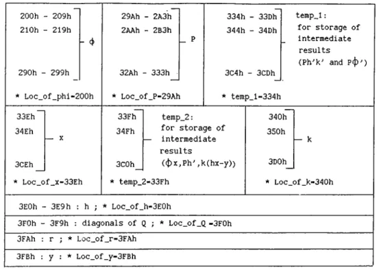
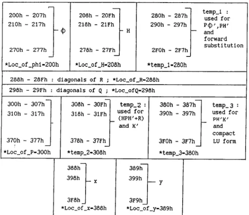
For a dynamic system up to ten states i. e. up to N = 10, all permanent data and intermediate results can be stored in on-chip data RAM . The scalars, vectors, matrices and intermediate results can be efficiently accommodated in on-chip RAM as shown in Figure 3.2. Incorporation of macros in Kalman fil ter algorithm is illustrated in Example 3.2. Note that the initialization part and the data acquisition parts are not included in this example as well as the subsequent examples.

Example 3.2

Consider the case when the dynamic system has N states where 2 < N < 10. Let us suppose that the N x N state transition matrix $ is stored at “Loc_of_phi” , N X N error covariance matrix

P

at “Loc_of_P” , N x N mea

surement noise covariance matrix Q at “Loc_of_Q” , N x 1 state vector x at “Loc_of_x” , the process noise variance R at “Loc_of_i‘” and the observation data y is stored at “Loc_of_y” . For storage of intermediate results, the loca tions “temp_l” and “ temp_2” as indicated by Figure 3.2 are used. The filter steps can be realized as :

(38)

CHAPTER 3. A GENERAL SOFTWARE FOR KALM AN FILTER 24 200h - 209h 210h - 219h - 4 290h - 299h * Loc_of_phi-200h 29Ah - 2A3h 2AAh - 2B3h 32Ah - 333h * Loc_of_P-29Ah 334h - 33Dh 344h - 34Dh 3C4h - 3CDh * temp_l-334h temp_l: for storage of intermediate results (Ph^k'' and Pcj)'') 33Eh 34Eh — X 3CEh * Loc_of_x-33Eh 33Fh 34Fh 3C0h temp_2: for storage of intermediate results ((¡^x^Ph" ,k(hx-y)) ^ temp_2-33Fh 340h 350h h- k 3D0h * Loc_of k-340h

3E0h - 3E9h : h ; * Loc_of_h-3E0h

3F0h - 3F9h : diagonals of Q ; * Loc_of_Q -3F0h

3FAh : r ; * Loc_of_r-3FAh 3FBh : y : Loc_of_y-3FBh

Figure 3.2: Storage Scheme for LTA and M P Y pair option

• find x { k + 1 I A:) = ^ x { k | k)

M tM tM ldd N , N , N , 1, Loc_of_phi, Loc_of_x, temp_2, 0, 0 ; temp-2 ■<—

M at.Copy iV, 1, temp_2, L oc.oL x ; x <— temp_2 • find P { k + l \ k ) = ^ P { k I k) ^^ + Q

M tM tM ldd N , N , N , N , Loc.oLphi, Loc_of_P, temp_l, 1, 0 ; temp_l <— [$P ]^ =

M tM tM ldd N , N , N , N , Loc.oLphi, temp_l, Loc_of_P, 0, 1 ; P <— $ P $ ^ (o n ly lower-half)

Mat-AorS TV, Loc-oLP, L oc.of.Q , 2 ; P f— 4 P $ ^ + Q Fill-Mat N , Loc-of-P ; fill the upper of P

• find k{k p i ) = P { k + l\ k)h^/{hP{k + 1 I + R) M tM tM ldd 1, N ^ N , N, Loc.oLh, Loc_oLP, temp_2, 1, 0 ; temp_2 <— \pPY = Ph^

VecVecMl TV, Loc.oLh, temp.2, 0, 0 ; (ACCH) <— lP~hF ScalAorS Loc-of-r ; (ACCH) ^ (ACCH )-l-P

VectMorD TV, temp_2, Loc.oLk, 1 ; k <— Ph^f(hPJi^ + R)

• find P ( k + 1 I ^ + 1) = P{ k + 1 I A:) — P { k + 1 | k)Wk'^{k -f 1)

VecVecMl TV, temp_2, Loc_of_k, temp_l, 1 ; tem p-l <— Ph^k^(on\y lower-half)

(39)

CHAPTER 3. A GENERAL SOFTWARE FOR KALM AN FILTER 25

Mat-AorS N , Loc_of_P, tem p.l, 1 ;

P

<— PhTk'^ Fill-Mat TV, L oc-of-P ; fill the upper-half of P

• find x { k -f 1 I Â; -f 1) = x{ k -|- 1 | A:) - k{k -|- l ) [ hx( k -1-1 | ^) - y]

VecVecMl N, Loc.oLh, Loc.oLx, 0, 0 ; (ACCH) <— hx — y ScalAorS Loc-of-y, 1 ; (ACCH) <— (A C C H )-?/

VectMorD N ^ Loc-oLk, temp-2, 0 ; temp_2 <— kÇhx — y) VectAorS A ’, Loc-of_x, temp-2, 1 ; x <— x — k(hx — y)

M A C Option

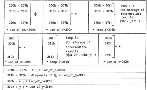
In this case, the fast multiply and accumulate instruction of TMS320C25 is exploited. To achieve this operands (i. e. vectors and matrices) are stored ei ther in program memory or data memory. For a filter that involves up to 8 state variables all the permanent data and intermediate results can be accom modated in on-chip RAM as shown in Figure 3.3. Note that CNFD/CNFP instruction moves the on-chip block BO back and forth between 200h of data memory and OFFOOh of program memory. The incorporation of macros into the standard Kalman filter is described in Example 3.3.

Example 3.3

The Exa.mple 3.2 is reconsidered again with the difference that in this case,

2 < N < 8. For this case, the filter steps can be summarized as :

• cnfp ; configure block BO as program memory • find

x(k

-1- 1 I A:) =

éx(k

|

k)

M tM tM lpd N , N , 1, 0FF00h-200h+Loc_of_phi, Loc_of_x, temp_2, 0, 0 ; temp-2 <—

M at-Copy N, 1, temp-2, Loc-oLx ;

x

<— temp-2 • find

P{k

+

l\k)

=

èP{k

I

k)è^

+

Q

M tM tM lpd N , N , N , 0FF00h-200h-fLoc-of-phi, Loc-of-P, temp-1, 1, 0 ; temp-1 <—

M tM tM lpd A , A , A,0FF00h-200h-t-Loc-of-phi, temp-1, Loc.of.P, 1, 1 ;

P

<— # P $ ^ (o n ly lower-half)

Mat-AorS A , Loc-of-P, Loc.of.Q, 2 ; P <— +

Q

Fill-Mat A , Loc-of-P ; fill the upper of P •

• find

k{k

+ 1) = P(yt -f-1 I

k)h'^/(hP{k

+ 1 I

k)h'^

-h P )

M tM tM lpd 1, A , A , OPPOOA — 200/i-fLoc-oLh, Loc-oLP, temp-2, 1, 0 ; temp-2 <— [ h P p = Ph^

(40)

VecVecMl N, OFFOOh — 200/i+Loc-of_h, temp_2, 0, 2 ; (ACCH) <— kPh^

ScalAorS Loc_of-r ; (ACCH) <— (A C C H )+ i?

VectMorD N, temp_2, Loc_of_k, 1 ; k <— PTF¡ (h P W + R) . find P(A: + 1 I A: + 1) = P(A: + 1 I A:) - P {k + 1 | + 1)

VecVecMl A ’, temp_2,Loc_of_k, temp_l, 1 ; temp-1 <— PWW{or\\y the lower-half)

Mat-AorS A , Loc-of-P, temp_l, 1 ; P <— P li^ W Fill-Mat A , L oc-of-P ; fill the upper-half of P

• find x{ k -f 1 I A: -f 1) = x{ k -f 1 | A:) - k{k -f- l)[hx{k -t- 1 | A;) — y] VecVecMl A , OFFOOh — 200/i-f-Loc_of_h, Loc-oLx, 0, 2

; (ACCH) <— h x - y

ScalAorS Loc_of_y, 1 ; (ACCH) ^ (ACCH) - y

VectMorD A , Loc_of_k, temp_2, 0 ; temp_2 <— k(hx — y) VectAorS A , Loc_of_x, temp_2, 1 ; x <— x — k(hx — y)

For 9 < n < 14, the on-chip RAM can not accommodate all permanent and temporary data. In this case, some of the data have to reside in external RAM . To keep the execution speed as fast as possible, only those data that are less involved in computations are stored in external memory.

200h - 207h 210h - 217h -(D 270h - 277h_ ' Loc_of_phi-200h 300h - 307h 310h - 317h - P 370h - 377h * Loc_of_P-300h 308h 318h 30Fh 3lFh 378h - 37Fh * temp_l-308h temp_l : for storage of intermediate results (Ph^k^P(f ') 380h 381h temp_2: 382h 390h 391h for storage of 392h - X intermediate - k results 3F0h 3Flh ((¡) x,Ph',k(hx-y) ) 3F2h

Loc_of _x-380h * temp_2-381h * Loc_of_k-382h

2F0h - 2F7h : h ; * Loc_of_h-2F0h

3F4h - 3FBh : diagonals of Q; * Loc_of_Q-3F4h

3FCh : r ; * Loc_of_r-3FCh 3FDh : y ; * Loc_of_y-3FDh

(41)

3.4.2 Vector Observation

When the observation is a vector quantity, the term [HPH' ^ + R) is no longer a scalar but a symmetric matrix. Hence inversion of an (M x M ) matrix is required if the standard Kalman filter is to be implemented. This problem can be overcome by sequential processing of observation vector. Another way to circumvent inversion is to solve Kalman gain K as & system of linear equations using either LU or Choleski factorization. In both the cases, matrix and vector multiplications are accomplished by “M AC option” i. e. we assume that the operands reside either in data memory or in program memory to maximize execution speed.

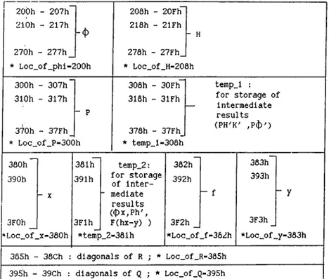
S eq u en tia l P r o c e s s in g :

For a system having up to 8 states and observation vector having up to 8 components i. e. up to A ” = 8, M = 8, all the permanent and intermediate results can be put into on-chip RAM . The storage scheme for this case is illustrated in Figure 3.4. The sequential processing can be very easily realized

r ~ . 200h - 207h 200h - 20Fh 210h - 217h 218h - 2lFh - H 270h - 2 7 7 h _ 270h - 27Fh_ * Loc_of_phi-200h * Loc_of_H-20flh 300h - 307h 308h - 30Fh temp_l : 310h - 317h 318h - 3lFh for storage of intermediate - P _results 370h - 37Fh_ 378h - 37Fh_ (PH^K' * Loc_of_P-300h * temp_l-308h 380h 381h temp_2: 382h 383h 390h 391h for storage of inter- 392h 393h - X “ mediate - f - y results ((f)x,Ph', 3F3h — 3F0h 3Flh F(hx-y) ) 3F2h _

*Loc_of__x-380h *temp_2-381h *Loc_of _f-362h *Loc_of__y-383h

385h -• 38Ch : diagonals of R ; * Loc_ofJR-385h

395h - 39Ch : diagonals of Q ; * Loc_of_Q-395h

Figure 3.4: S to r a g e S ch em e fo r S equ en tial P r o c e s s in g , N = 8

using the special macro “ Seq_Proc” which finds the filtered estimates of state vector x{ k 1 I k 1) and error covariance matrix P (A :-t-ljA :-| -l). The use

Implementation of a state-space Kalman filter on a digital signal processing microprocessor

s у BMITTEp. T ö ■

·ΤΗΙ^" ·θ £PÄ^TMBp'r::

P

IMPLEMENTATION OE A STATE-SPACE KALMAN

FILTER ON A DIGITAL SIGNAL PROCESSING

MICROPROCESSOR

-By

M. Khaledul Islam

August 1990

ABSTRACT

IMPLEMENTATION OF A STATE-SPACE KALM AN

FILTER ON A DIGITAL SIGNAL PROCESSING

MICROPROCESSOR

M. Khaledul Islam

M.S. in Electrical and Electronics Engineering

Supervisor: Asst. Prof. Dr. Gürhan Şaplakoğlu

August 1990

ÖZET

DURUM UZAYI KALMAN FİLTRESİNİN BİR SAYISAL

İŞARET İŞLETİCİSİNDE GERÇEKLEŞTİRİLMESİ

M. Khaledul İslam

Elektrik ve Elektronik Mühendisliği Bölümü Yüksek Lisans

Tez Yöneticisi; Yrd. Doç. Dr. Gürhan Şaplakoğiu

Ağustos 1990

ACKNOWLEDGMENT

Contents

List of Figures

N = 8

LIST OF FIGURES

Q

R —

Q =

R =

e =

a =

Qy R

k.

Qy Ry

Qy

R

Q

List of Tables

N = 8^ 2 < M < 8

N = 8, 2 < M < 8

Chapter 1

INTRODUCTION

1.1

The State-Space Kalman Filter

iy

1.2

T M S 320 Digital Signal Processor Family

1

1.3

W h y Fixed-Point Processor ?

1.4

Real-time Kalman Filter on a Fixed-point Digital

Signal Processor

Chapter 2

A R EVIEW OF THE K A LM A N FILTER

ALGORITHMS

2.1

The Kalman Filter

2.1.1

Notational Convention

2.1.2

The Algorithms

(

2

.

1

)

(2.2)

Qi

i = j

i = j

i.

2

12

2.2