https://doi.org/10.1007/s40096-021-00401-9
ORIGINAL RESEARCH
An operational matrix method to solve linear Fredholm–Volterra
integro‑differential equations with piecewise intervals
Yalçın Öztürk1 · Mustafa Gülsu2
Received: 18 June 2020 / Accepted: 5 April 2021 / Published online: 19 April 2021 © Islamic Azad University 2021
Abstract
In recent times, operational matrix methods become overmuch popular. Actually, we have many more operational matrix methods. In this study, a new remodeled method is offered to solve linear Fredholm–Volterra integro-differential equations (FVIDEs) with piecewise intervals using Chebyshev operational matrix method. Using the properties of the Chebyshev polynomials, the Chebyshev operational matrix method is used to reduce FVIDEs into a linear algebraic equations. Some numerical examples are solved to show the accuracy and validity of the proposed method. Moreover, the numerical results are compared with some numerical algorithm.
Keywords Piecewise Fredholm–Volterra equations · Operational matrix method · Chebyshev polynomials
Introduction
Integro-differential equations are very important to model a real world phenomenons. Integro-differential equations usu-ally are a combination of differential, Fredholm and Volterra integral equations. These type of equations arise in applied sciences such as wave mechanics, heat conduction, medi-cine, chemistry, astronomy, electrostatics, etc.[1–4]. Hence, the solutions of these type equations gain prominence to find out the behavior of modeling.
These type of equations usually difficult to solve exactly since it has many parts of differential, Fredholm and Volterra integral. The Fredholm–Volterra integro differential equa-tions (FVIDEs) have been widely studied by many more authors to obtain the numerical solutions. In [5], authors introduced an efficient Bernoulli matrix method to solve high order linear Fredholm integro differential equation with piecewise intervals. In [6], an efficient Bernoulli collocation method has been developed to gain numerical solution such an equations. In [7], Acar and Daşçıoğlu developed a projec-tion method based on Bernstein polynomials for soluprojec-tion of
linear FVIDEs. In [8], Kürkçü, Aslan and Sezer presented a collocation method using hybrid Dickson and Taylor poly-nomials to obtain the numerical solutions of FVIDEs.
In [9], Yüksel et al. obtained a Chebyshev polynomial method for high-order linear Fredholm–Volterra integro-differential equations. In [10], Ebrahimi and Rashidinia produced a cubic B-spline approach by using the New-ton–Cotes formula for FVIDEs. Also, we have many more studies in literature such as Dickson polynomials solution [11], Lucas polynomials solution [12], a polynomial solution [13], the backward substitution method [14], He’s homotopy perturbation method [15], Mott polynomials solution [16], Laguerre polynomial solution [17], Taylor series solution [18], the semi orthogonal B-spline wavelet solution [19], a Tau method [20] and the power series method [21].
In this study, a operational matrix method is presented to solve the linear FVIDEs with piecewise intervals of the following form
with mixed conditions
(1) m ∑ k=0 Pk(x)y(m)(x) + p ∑ m=0 𝜇m x ∫ cm Vm(x, t)y(t)dt + q ∑ n=0 𝜆n bn ∫ an Fn(x, t)y(t)dt = f (x) * Mustafa Gülsu [email protected]
1 Ula Ali Koçman Vocational School, Muğla Sıtkı Koçman
University, Muğla, Turkey
where the parameter 𝜆s , 𝜇r and 𝜆s are constants.Pk(x) and
f(x) are known and belong to L2[0, 1] . We desire to find the unknown function y(x). For this purpose, the approximation series are defined by
where N is any positive integer and T∗
r(x) , r = 0, 1, … , N denote the shifted Chebyshev polynomials [22] and N ≥ m.
This paper is organized as follows: Definitions and some properties of the Chebyshev polynomials are mentioned in Sect. 2. Section 3 is introduced representation of the matrix form of differential, Fredholm and Volterra integral part in Eq. (1). The numerical method establishes in Sect. 4. In Sect. 5, several treatments are presented. In Sect. 6, a con-clude adds the paper. All computations have been calculated by Maple13. Figures have been plotted by Matlab.
The operational matrix method has been investigated by some author [23–29]. In these studies, this method is suc-cessfully solved the Abel equation, fractional integro differ-ential equations, the Lane-Emden equation, fractional order differential equations and nonlinear Volterra integro differ-ential equations. All above issues motivate us to introduce an operational matrix method for FVIDEs.
Chebyshev polynomials
It is well known that the fundamental theorem of approxi-mation is called Weierstrass Theorem which says us any continuous function can be approximated uniformly by poly-nomials (See [30] for details). If you need a polynomial to make an approximation, you should choose an ordinary Fou-rier series (See [31] for details). The first type Chebyshev polynomial is a Fourier cos series.
Describe Tn(x) which is called the Chebyshev functions family by formula, for n ≥ 0
Theorem 1 The family of Tn(x) satisfy the following
properties. a. The degree of Tn(x) is n. b. For n ≥ 1 , Tn+1(x) = 2xTn(x) − Tn−1(x). c. Tn(x) = 2n−1xn+ ⋯ (2) m−1 ∑ k=0 (aiky(k)(a) + biky(k)(b) + ciky(k)(c)) = 𝛼i, i= 0, 1, … , m − 1. (3) yN(x) = N ∑ r=0 arTr∗(x), x∈ [0, 1],
Tn(x) = cos(n arc cosx), x∈ [−1, 1]
d. (Ti, Tj)w=∫ 1
−1w(x)Ti(x)Tj(x)dx = 0 , i ≠ j w h e re
w(x) = (1 − x2
)−1∕2 is called weight function.
e. The roots of the Tn+1(x) are xk= cos (
(2k+1)𝜋
2(n+1)) , 0 ≤ k ≤ n
which is called the Chebyshev nodes to compute inter-polating approximations for continuous functions. Proof: See [22].
Theorem 2. Let f ∈ Cn+1[−1, 1] and the n degree
polyno-mial pn(x) interpolate to f . Using the Chebyshev nodes, we
have.
Proof: See [22].
Theorem 3. Let yN(x) be an approximation to y(x). The
truncation error ET(N) can be bounded by the following
inequality. If.
then
Proof: See [22].
Since Tn(x) is a function of cos 𝜃, −1 ≤ Tn(x)≤ 1. . If we want to change the interval of Tn(x) as [0, 1], we can use the transformation y = 2x − 1. Then the Chebyshev polynomi-als become
which is called the shifted Chebyshev polynomials of the first kind.
Some properties can be written as [22]: (i)
are roots of T∗ n+1(x).
(ii) where ∑′
denotes a sum whose first term is halved. Clearly, Theorems 1, 2 and 3 can be converted for the shifted Chebyshev polynomials.
(4) ‖ ‖ f − pn‖ ‖∞≤ 1 2n(n + 1)! ‖ ‖ ‖ f(n+1)‖ ‖ ‖∞ (5) yN(x) = N ∑ r=0 arTr∗(x) ET(N) = ‖ ‖ y(x) − yN(x)‖ ‖≤ ∞ ∑ r=N+1 | | ar| | Tn∗(x) = Tn(y) = Tn(2x − 1) (6) xi= 1 2 ( 1+ cos( (2(n − i) + 1)𝜋 2(n + 1) )) , i= 0, 1, … , n (7) xn= 2−2n+1 n ∑ k=0 � ( 2n k ) Tn−k∗ (x), 0≤ x ≤ 1
Matrix relations
In this section, the matrix–vector form of the each part of Eq. (1) is introduced by using Eqs. (3) and (6).
Matrix representation of differential part
To obtain the numerical results of Eq. (1), we construct the fundamental matrix–vector relations. These relations help us when we use operational method. Firstly, we suppose that the numerical solution can be written in the shifted first kind Chebyshev series form. The matrix–vector form the approximate solution and its derivatives can be written where
From Eq. (6), we get the following matrix relation where
Since the matrix D is invertible, Eq. (9) can be clearly written
and
The following relation give us Y(k)(x) in terms of Y(x) (8) yN(x) = 𝐓∗(x)𝐀, y(k)N (x) = 𝐓∗(k)(x)𝐀, k= 0, … , m 𝐓∗(x) = [T∗ 0(x) T ∗ 1(x) ⋯ T ∗ N(x)], 𝐀= [a0a1… aN] T (9) (𝐘(x))T = 𝐃(𝐓∗(x))T and 𝐘(x) = 𝐓∗(x)𝐃T 𝐘(x) = [ 1 x … xN] 𝐃= ⎡ ⎢ ⎢ ⎢ ⎢ ⎢ ⎢ ⎢ ⎢ ⎢ ⎢ ⎢ ⎢ ⎢ ⎢ ⎢ ⎢ ⎣ 20 � 0 0 � 0 0 0 … 0 2−2 � 2 1 � 2−1 � 2 0 � 0 0 … 0 2−4 � 4 2 � 2−3 � 4 1 � 2−3 � 4 0 � 0 … 0 2−6 � 6 3 � 2−5 � 6 2 � 2−5 � 6 1 � 2−5 � 6 0 � … 0 ⋮ ⋮ ⋮ ⋮ ⋱ ⋮ 2−2N � 2N N � 2−2N+1 � 2N N− 1 � 2−2N+1 � 2N N− 2 � 2−2n+1 � 2N N− 3 � … 2−2N+1 � 2N 0 � ⎤ ⎥ ⎥ ⎥ ⎥ ⎥ ⎥ ⎥ ⎥ ⎥ ⎥ ⎥ ⎥ ⎥ ⎥ ⎥ ⎥ ⎦ (10) 𝐓∗(x) = 𝐘(x)(𝐃−1)T (11) (𝐓∗(x))(k)= 𝐘(k)(x)(𝐃−1)T, k= 0, … , m. (12) 𝐘(1)(x) = 𝐘(x)𝐁T where
If the obtained the matrix forms Eqs. (11) and (13) are substituted into (8), the approximate solution function
yN(x) = ∑N
n=0anTn∗(x) can be transformed into the follow-ing matrix form
Matrix representation of Volterra and Fredholm integral part
In this section, we try to find matrix–vector form Volterra and Fredholm integral part in Eq. (1). For this purpose, sup-pose that the kernel function Vm(x, t) can be written as:
and the matrix form of the Vm(x, t) become where (13) 𝐘(2)(x) = 𝐘(1)(x)𝐁T= 𝐘(x)(𝐁T)2 ⋮ 𝐘(k)(x) = 𝐘(k)(x)𝐁T= 𝐘(x)(𝐁T)k 𝐁= ⎡ ⎢ ⎢ ⎢ ⎢ ⎢ ⎣ 0 0 0 … 0 1 0 0 … 0 0 2 0 … 0 … … … … … 0 0 0 N 0 ⎤ ⎥ ⎥ ⎥ ⎥ ⎥ ⎦ (14) y(k)N (x) = 𝐘(x)(𝐁T )k(𝐃T)−1𝐀, k= 0, … , m (15) Vm(x, t) = N ∑ r=0 kmr(x)Tr∗(t). (16) Vm(x, t) = 𝐊m(x)𝐓T(t) 𝐊m(x) = [ km0(x) km1(x) km2(x) ⋯ kmN(x) ]
Using Eqs. (14) and (16), we obtain the following matrix–vector form of the Volterra integral part
Now, assume that the kernel function Fn(x, t) can be writ-ten as:
Then the matrix form of the kernel function Fn(x, t) become
where
Using Eqs. (14) and (19), we obtain the following matrix–vector form of the Fredholm integral part
Method of solution
In this chapter, the matrix–vector form of Eq. (1) and the operatinal matrix method are assembled to erect the numer-ical method. Firstly, we have to change the form of f (x) into a matrix–vector form. The matrix form of f (x) can be considered
The obtained matrix–vector forms of differential part, Volterra and Fredholm integral part are put into Eq. (1), we obtain the following matrix–vector equation
(17) ⎡ ⎢ ⎢ ⎣ p � m=0 𝜇m x ∫ cm Vm(x, t)y(t)dt ⎤ ⎥ ⎥ ⎦ = p � m=0 𝜇m x ∫ cm 𝐊 m(x)𝐃 −1𝐘T(t)𝐘(t)(𝐃T)−1Adt (18) Fn(x, t) = N ∑ r=0 fnr(x)Tr∗(t) (19) Fn(x, t) = 𝐅n(x)𝐓 T (t) Fn(x) = [ fn0(x) fn1(x) fn2(x) ⋯ fnN(x) ] (20) ⎡ ⎢ ⎢ ⎣ q � n=0 𝜆n bn ∫ an Fn(x, t)y(t)dt ⎤ ⎥ ⎥ ⎦ = q � n=0 𝜆n bn ∫ an 𝐅 n(x)𝐃−1𝐘T(t)𝐘(t)(𝐃T)−1𝐀dt (21) f(x) ≈ 𝐆T𝐘(x)(𝐃T)−1 (22) m ∑ k=0 𝐏 k(x)𝐘(x)(𝐁 T )k(𝐃T)−1𝐀 + p ∑ m=0 𝜇m x ∫ cm 𝐊 m(x)𝐃 −1𝐘T(t)𝐘(t)(𝐃T)−1𝐀dt + q ∑ n=0 𝜆n bn ∫ an 𝐅 n(x)𝐃 −1𝐘T(t)𝐘(t)(𝐃T)−1𝐀dt≈ 𝐆T𝐘(x)(𝐃T)−1
Thus, the residual function RN(x) can be gained the fol-lowing equation:
Using operational matrix method idea, we gain (N − m + 1) linear equations as follows:
where w(x) = (x − x2)−1∕2 . The m-times initial conditions are obtained by
Hence, we have ( N + 1 ) times linear equations including the unknown coefficients in Eq. (3). If we figure out these linear equations by aid of Maple 13, the approximate solu-tion yN(x) can be obtained from Eq. (3).
Error estimation and convergence analysis
Now, we will discuss error estimation and convergence analysis.
Theorem: Let assume that.
(which is the best approximation to y(x) ) are the shifted
Chebyshev polynomials expansion of the exact solution y(x) ∈ CN+1 andis the approximate solution the obtained by
proposed method. Then, we have
(23) RN(x) ≈ m ∑ k=0 𝐏 k(x)𝐘(x)(𝐁 T )k(𝐃T)−1𝐀 + p ∑ m=0 𝜇m x ∫ cm 𝐊 m(x)𝐃−1𝐘T(t)𝐘(t)(𝐃T)−1𝐀dt + q ∑ n=0 𝜆n bn ∫ an 𝐅 n(x)𝐃 −1𝐘T(t)𝐘(t)(𝐃T)−1𝐀dt− 𝐆T𝐘(x)(𝐃T)−1 (24) ⟨RN(x), Tn∗(x) ⟩ w= 1 ∫ 0 w(x)RN(x)Tn∗(x)dx = 0, n= 0, 1, … , N − m (25) m−1 ∑ k=0 (aik𝐘(a)(𝐁𝐓)k(𝐃T)−1+ bik𝐘(b)(𝐁𝐓)k(𝐃T)−1 +cik𝐘(c)(𝐁 𝐓 )k (𝐃T )−1)𝐀 = 𝛼 i yB(x) = ∞ ∑ r=0 brTr∗(x) ≅ N ∑ r=0 brTr∗(x) + ∞ ∑ r=N+1 br yN(x) = N ∑ r=0 arTr∗(x) (26) � � y(x) − yN(x)� �2≤ 1 22N+1 � � � y(N+1)(x)�� �∞ + � 3𝜋 8 ‖B − A‖2
where
Proof: Firstly, the following inequality is held.
From Eq. (4), we have the following inequality
and we have
On the other hand, since the approximate solution yN(x) is the approximate solution of Eq. (1), then Eq. (1) must be approximately satisfied by the function yN(x).
The following comparison strongly advise by [20]:
A=[ a0 a1 ⋯ aN ] and B=[ b0 b1 ⋯ bN]. ‖ ‖ y(x) − yN(x)‖ ‖2 ≤ ‖ ‖ y(x) − yB(x)‖ ‖2+ ‖‖ yB(x) − yN(x)‖ ‖2 . � � y(x) − yB(x)� �2 = ⎛ ⎜ ⎜ ⎝ 1 � 0 w(x)� � y(x) − yB(x)� � 2 dx ⎞ ⎟ ⎟ ⎠ 1∕2 ≤⎛⎜ ⎜ ⎝ 1 � 0 � 1 22N+1(N + 1)! � � � y(N+1)(x)�� �∞ �2 dx ⎞ ⎟ ⎟ ⎠ 1∕2 = 1 22N+1(N + 1)! � � � y(N+1)(x)�� �∞ � � yB(x) − yN(x)� �2 = ⎛ ⎜ ⎜ ⎝ 1 � 0 �N � r=0 (br− ar)Tr∗(x) �2 dx ⎞ ⎟ ⎟ ⎠ 1∕2 ≤⎛⎜ ⎜ ⎝ 1 � 0 �N � r=0 (br− ar) 2 �� N � r=0 � �T ∗ r(x)�� 2 � dx ⎞ ⎟ ⎟ ⎠ 1∕2 = � N � r=0 (br− ar) 2 �1∕2 ⎛ ⎜ ⎜ ⎝ N � r=0 1 � 0 � � Tr∗(x)� � 2 dx ⎞ ⎟ ⎟ ⎠ 1∕2 = � 3𝜋 8 ‖B − A‖. (27) | | | | | | | m ∑ k=0 Pk(x)y(m)(x) + p ∑ m=0 𝜇m x ∫ cm Vm(x, t)y(t)dt + q ∑ n=0 𝜆n bn ∫ an Fn(x, t)y(t)dt = f (x) | | | | | | | ≈ 0 (28) EN= m ∑ k=0 Pk(x)y(m)(x) + p ∑ m=0 𝜇m x ∫ cm Vm(x, t)y(t)dt + q ∑ n=0 𝜆n bn ∫ an Fn(x, t)y(t)dt − f (x)
which is called error estimation function.
Illustrative examples
In this section, we apply our method some examples to check the accuracy and effectiveness of the method. In examples, some comparisons are dispalyed by below fundamental error types:
1. Absolute error ( Ne ) is defined by:
where y(x) are the exact solution and yN(x) denote the approximate solution.
2. relN is relative error which is defined by
Example 1. Firstly, we apply our method to following the linear FVIDE with piecewise intervals subject to y(0) = 1,
y�(0) = −2, y��(0) − 2y�(0) = 7.
where
The exact solution is y(x) = (1 − x)e−x. Then, we have
Ne(x) = | | y(x) − yN(x)| | , x∈ [0, 1] relN= || y(x) − yN(x)| | |y(x)| , x∈ [0, 1] y���(x) − y�(x) + x ∫ 0 xty(t)dt + 1∕2 ∫ 1∕4 (1 − t2 x2)y(t)dt − 1 ∫ 1∕2 (1 − t)y(t)dt = f (x) f(x) = (−2 + x + x2+ x3)ex+ 0.0861606918 − 0.014742845x2 P0(x) = 0, P1(x) = −1, P2(x) = 0, P3(x) = 1
If these values and functions are put into Eq. (24), we have the following approximate solutions for various N values
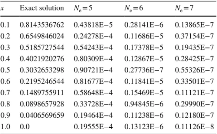
Comparison of these approximate solutions and exact solution are presented in Table 1. Table 2 gives us the com-parison of the relative errors. Figure 1 shows us comparison of absolute errors, Fig. 2 and 3 display error estimation func-tions and relative error funcfunc-tions, respectively. These figures say that if the N values are increased, the absolute values and relative errors are decreased. Hence, the numerical results are more close with the exact solution.
Example 2. Let us consider the following linear Fredholm integro-differential equation with piecewise intervals [5]
If the above numerical algorithm is applied, we have the following numerical solutions
Also, this problem has been solved by Bernoulli matrix method (BMM) [5]. Table 3 and Fig. 4 show the comparison of Present Method and BMM. From Fig. 4, our numerical results are better than BMM.
𝜆1= 1, F0(x, t) = xt, c0 = 0 𝜇1= 1, 𝜇2= −1, V0(x, t) = 1 − x 2t2 , V1(x, t) = 1 − t, a0= 1∕4, b0= 1∕4, a1= 1∕2, b1= 1 y 5(x) = 1 − 2x + 3 2 x2− 0.6605636x3 + 0.18906493x4 − 0.028481763x5 y 6(x) = 1 − 2x + 3 2 x2 − 0.66617680x3 + 0.20580958x4 − 0.0452840x5+ 0.0055757467x6 y7(x) = 1 − 2x +3 2x 2 − 0.66663491x3 + 0.2080941625x4 − 0.0493161690x5 + 0.008770421x6 − 0.000912765x7 y���(x) = ex− x − 4 1∕4 ∫ 0 ex+ty(t)dt + 2 1∕2 ∫ 0 xety(t)dt − 1 ∫ 0 et−xy(t)dt, y(0) = 1, y�(0) = −1, y��(0) = 1 y6(x) = 1 − x + 0.5x2− 0.166602262x3 + 0.0413353094x4− 0.00770776517x5 + 0.00085415183x6 y 8(x) = 1 − x + 0.5x 2 − 0.166664113x3 + 0.0416480144x4 − 0.00828084359x5 + 0.001315741562x6 − 0.0001454724104x7+ 0.61145088e − 5x8
Example 3. Let us consider the following linear FVIDE with
piecewise intervals. y��(x) − (1 − x)y�+ y = f (x) + 1∕2 ∫ 0 xty(t)dt + 1 ∫ 1∕2 (1 − xt)y(t)dt + x ∫ 0 (xt2 − x2 t)y(t)dt, y(0) = 0, y�(0) = 0. , I f w e c h o o s e f (x) = 24x3− 12x2− 10x4 +6x5− 1 48x+ 19 640+ 1 56x 9− 1 42x
8, the exact solution is x5 − x4
. When solving this example by mention method, we get the exact solution for N = 5.
Example 4. Let us consider the following equation [33]
with nonlocal boundary condition
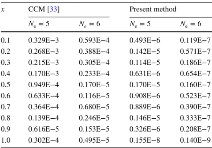
The exact solution of this problem is y(x) = ex. In Table 4, we compare our results with the existing method Chebyshev collocation method [33]. The comparison of these results in Fig. 5 and Table 4 shows that our numerical results have a perfect harmony with the exact solution.
Example 5. Let us consider the following Fredholm integro differential equation [7, 34]:
The exact solution is y(x) = cos(x). The Bernstein projec-tion method (BPM), the variaprojec-tional iteraprojec-tion method (VIM) and the proposed method (PM) are compare in Table 5. It can be observed from Table 5 that PM has less errors com-pare with BPM and VIM.
y�(x) − y(x) = −ex− e + 2 + 1 ∫ 0 y(t)dt + x ∫ 0 y(t)dt y(0) + 1 ∫ 0 y(t)dt = e y���(x) = sin(x) − x − 𝜋∕2 ∫ 0 xty�(t)dt and y(0) = 1, y�(0) = 0, y��(0) = −1
Steps of Solutions
In this section, steps of solution have been presented the given numerical method. Maple program is used in this arti-cle for run it. Readers can apply the algorithm any computer program.
Algorithm:
(a) Input values and function should be determined N , 𝜇m , 𝜆n , Pk(x) ,
Vm(x, t) , Fn(x, t) , f (x) , cm , an , aik , bik , cik , a , b , c and 𝛼i. (b) Take suitable matrices for A , D , Y(x) , B , Km , Fn,G
(c) Using Eqs.(24)-(25), construct the RN(x) and (N − m) linear
equa-tions from mixed condiequa-tions
(d) Solve the obtained linear equations on (c) with conditions (e) Substituting all coefficients into Eq. (3), this is approximate
solu-tion
Conclusion
The operational matrix method is treated as accurate, effec-tive and plain method to gain numerical solutions of the FVIDEs. This method is based on polynomial approxima-tion and basic operaapproxima-tional method. By the aid of operaapproxima-tional matrices, the all terms of Eq. (1) reduce to a linear alge-braic equations. The present method has some consider-able advanteges. Since the entry of operational matrices is
Table 1 Error values of Ex. 1 for the x value
x Exact solution Ne = 5 Ne = 6 Ne = 7
0.1 0.8143536762 0.43818E−5 0.28141E−6 0.13865E−7 0.2 0.6549846024 0.24278E−4 0.11686E−5 0.37154E−7 0.3 0.5185727544 0.54243E−4 0.17378E−5 0.19435E−7 0.4 0.4021920276 0.80309E−4 0.12867E−5 0.28425E−7 0.5 0.3032653298 0.90721E−4 0.27736E−7 0.55326E−7 0.6 0.2195246544 0.81677E−4 0.11841E−5 0.33501E−7 0.7 0.1489755911 0.58648E−4 0.15469E−5 0.11121E−7 0.8 0.0898657928 0.33728E−4 0.94845E−6 0.29990E−7 0.9 0.0406569659 0.19464E−4 0.11238E−6 0.12180E−7 1.0 0.0 0.19555E−4 0.13123E−6 0.11126E−8
Fig. 2 Comparison of error estimation functions in Ex. 1
Table 2 Some values of relative
error N relN
5 0.4787E−4
6 0.2765E−5
7 0.3148E−6
Fig. 1 Comparison of absolute errors in Ex. 1
zeroes, the present method has lower operation count and shorter computation time. These advantages bring about less cumulative truncation errors. Also, from Ex.3, if the exact solution is a polynomial, our numerical method give
us this polynomial. The proposed method presents us more convenient numerical results than compared methods from Exs. 2, 4 and 5.
Table 3 Numerical comparisons for Ex. 2
x BMM [5] Present method
Ne= 6 Ne= 8 Ne= 6 Ne= 8
0.1 0.31830E−8 0.29967E−10 0.35862E−7 0.114469E−8 0.2 0.22137E−7 0.506946E−9 0.15016E−6 0.332729E−8 0.3 0.37989E−7 0.265453E−8 0.22456E−6 0.247957E−8 0.4 0.12781E−6 0.898136E−8 0.16520E−6 0.103320E−8 0.5 0.11175E−5 0.254436E−7 0.37140E−8 0.353077E−8 0.6 0.45985E−5 0.684357E−7 0.17051E−6 0.271857E−8 0.7 0.14152E−4 0.182284E−6 0.22607E−6 0.14506E−10 0.8 0.36567E−4 0.476192E−6 0.15097E−6 0.142662E−8 0.9 0.83519E−4 0.119350E−5 0.40120E−7 0.486501E−9 1.0 0.17390E−3 0.283062E−5 0.74450E−8 0.266051E−9
Fig. 4 Comparison of PM and BMM in Ex. 2
Table 4 Numerical comparisons for Ex. 4
x CCM [33] Present method
Ne= 5 Ne= 6 Ne= 5 Ne= 6
0.1 0.329E−3 0.593E−4 0.493E−6 0.119E−7 0.2 0.268E−3 0.388E−4 0.142E−5 0.571E−7 0.3 0.215E−3 0.305E−4 0.114E−5 0.186E−7 0.4 0.170E−3 0.233E−4 0.631E−6 0.654E−7 0.5 0.949E−4 0.170E−5 0.170E−5 0.160E−7 0.6 0.633E−4 0.116E−5 0.908E−6 0.523E−7 0.7 0.364E−4 0.680E−5 0.889E−6 0.390E−7 0.8 0.139E−4 0.246E−5 0.146E−5 0.333E−7 0.9 0.616E−5 0.153E−5 0.326E−6 0.208E−7 1.0 0.302E−4 0.495E−5 0.155E−8 0.140E−9
Fig.5 Comparison of PM and CCM
Table 5 Comparison of BPM,
VIM and PM x BPM [7] VIM [34] PM
Ne= 6 Ne= 12 k = 5 k = 10 Ne= 6 Ne= 12
0.2 6.6E−8 8.2E−15 2.1E−5 6.3E−7 1.03E−7 6.29E−13
0.4 6.6E−7 5.6E−14 3.4E−4 1.0E−5 3.01E−8 1.03E−14
0.6 2.2E−6 1.9E−13 1.7E−3 5.1E−5 6.57E−7 5.24E−13
0.8 5.7E−6 4.7E−13 5.4E−2 1.6E−4 1.80E−6 1.65E−13
References
1. Delves, L.M., Mohamed, J.L.: Computational Methods for Inte-gral Equations. Cambridge University Press, Cambridge (1985) 2. Agarwal, R.P. (ed.): Contributions in Numerical Mathematics.
World Scientific Publishing, Singapore (1993)
3. Agarwal, R.P. (ed.): Dynamical Systems and Applications. World Scientific Publishing, Singapore (1995)
4. Wazwaz, A.M.: A First Course in Integral Equations. World Sci-entifics, Singapore (1997)
5. Bhrawy, A.H., Tohidi, E., Soleymani, F.: A new Bernoulli matrix method for solving high-order linear and nonlinear Fredholm inte-gro-differential equations with piecewise intervals. Appl. Math. Comp. 219, 482–497 (2012)
6. Biçer, G.G., Öztürk, Y., Gülsu, M.: Numerical approach for solv-ing linear Fredholm integro-differential equation with piecewise intervals by Bernoulli polynomials. Inter. J. Comp. Math. 95, 2100–2111 (2018)
7. Acar, N.İ, Daşçıoğlu, A.: A projection method for linear Fred-holm-Volterraintegro differential equations. J. Taibah Univ. Sci.
13(1), 644–650 (2019)
8. Kürkçü, Ö.K., Aslan, E., Sezer, M.: A novel collocation method based on residual error analysis for solving integro differential equations using hybrid Dickson and Taylor polynomials. Sains Malaysiana 46, 335–347 (2017)
9. Yüksel, G., Gülsu, M., Sezer, M.: A Chebyshev polynomial approach for high-order linear Fredholm-Volterra integro-differ-ential equations. GU J Sci. 25, 393–401 (2012)
10. Ebrahimi, N., Rashidinia, J.: Spline collocation for Fredholm and Volterra integro-differential equations. Int. J. Math. Model. Com-put. 4(3), 289–298 (2014)
11. Kürkçü, Ö.K., Ersin, A., Sezer, M.: A numerical approach with error estimation to solve general integro-differential difference equations using Dickson polynomials. Appl. Math. Comput. 276, 324–339 (2016)
12. Gümgüm, S., Baykuş, N., Savaşaneril, N., Kürkçü, Ö., Sezer, M.: A numerical technique based on Lucas polynomials together with standard and Chebyshev-Lobatto collocation points for solving functional integro-differential equations involving variable delays. Sakarya Univ. J. Sci. 22(6), 1659–1668 (2018)
13. Kurt, N., Sezer, M.: Polynomial solution of high-order linear Fred-holm integro-differential equations with constant coefficients. J. Franklin Inst. 345, 839–850 (2008)
14. Reutskiy, S.Y.: The backward substitution method for multipoint problems with linear Volterra-Fredholm integro-differential equa-tions of the neutral type. J. Comput. Appl. Math. 296, 724–738 (2016)
15. Dehghan, M., Shakeri, F.: Solution of an integro-differential equa-tion arising in oscillating magnetic field using He’s homotopy per-turbation method. Prog. Electromagnet. Res. PIER 78, 361–376 (2008)
16. Kürkçü, Ö.K.: A numerical method with a control parameter for integro differential delay equations with state dependent bounds via generalized Mott polynomials. Math. Sci. 14, 43–52 (2020)
17. Gürbüz, B., Sezer, M., Güler, C.: Laguerre collocation method for solving Fredholm integro-differential equations with functional arguments. J. Appl. Math. 682398 (2014)
18. Gülsu, M., Sezer, M.: Taylor collocation for the solution of sys-tems of high-order linear Fredholm-Volterraintegro-differential equations. Int. J. Comput. Math. 83, 429–448 (2006)
19. Sahu, P.K., Saha Ray, S.: Numerical solutions for the system of Fredholm integral equations of second kind by a new approach involving semiorthogonal B-spline wavelet collocation method. Appl. Math. Comput. 234, 368–379 (2014)
20. Shahmorad, S.: Numerical solution of the general form linear Fredholm-Volterra integro differential equations by the Tau method with an error estimation. App. Math. Comput. 167, 1418–1429 (2005)
21. Turkyilmazoglu, M.: An effective approach for numerical solu-tions of high-order Fredholm integro-differential equasolu-tions. Appl. Math. Comput. 227, 384–398 (2014)
22. Mason, J.C., Handscomb, D.C.: Chebyshev Polynomials. Chap-man and Hall/CRC, New York (2003)
23. Vanani, S.K., Aminataei, A.: Operational Tau approximation for a general class fractional integro-differential equations. Comp. Appl. Math. 30(3), 655–674 (2011)
24. Öztürk, Y., Gülsu, M.: An operational matrix method for solving Lane-Emden equations arising in astrophysics. Math. Methods App. Sci. 37, 2227–2235 (2014)
25. Babolian, E., Fattahzadeh, F.: Numerical solution of differential equations by using Chebyshev wavelet operational matrix of inte-gration. Appl. Math. Comp. 188, 417–425 (2007)
26. Saadatmandi, A.: Mehdi Dehghan, A new operational matrix for solving fractional-order differential equations. Comp. Math. Appl.
59, 1326–1336 (2010)
27. Öztürk, Y.: Numerical solution of systems of differential equations using operational matrix method with Chebyshev polynomials. J. Taibah Uni. Scie. 12(2), 155–162 (2018)
28. Öztürk, Y., Gülsu, M.: Numerical solution of Abel equation using operational matrix method with Chebyshev polynomials. Asian-Eur. J. Math. 10(3), 175053 (2017)
29. Öztürk, Y., Gülsu, M.: An operational matrix method for solving a class of nonlinear Volterra integro-differential equations by opera-tional matrix method. Inter. J. Appl. Comput. Math. 3, 3279–3294 (2017)
30. Rivlin, T.J.: Introduction to the Approximation of Functions. Lon-don (1969)
31. Body, J.P.: Chebyshev and fourier spectral methods. University of Michigan, New York (2000)
32. Epperson, J.F.: An Introduction to Numerical Methods and Analy-sis. Wiley & Sons, Inc., Hoboken, New Jersey (2013)
33. Gülsu, M., Öztürk, Y.: On the numerical solution of linear Fred-holm-Volterra integro differential difference equations with piece-wise intervals. Appl. Appl. Math. Int. J. 7(2), 556–570 (2012) 34. Shang, X., Han, D.: Application of the variational iteration
method for solving n-th order integro differential equations. J. Comput. Appl. Math. 234, 1442–1447 (2010)