Identifying key developers using artifact traceability graphs

Identifying Key Developers using Artifact Traceability Graphs

H. Alperen Çetin

Eray Tüzün

ABSTRACT

Developers are the most important resource to build and maintain software projects. Due to various reasons, some developers take more responsibility, and this type of developers are more valuable and indispensable for the project. Without them, the success of the project would be at risk. We use the termkey developers for these essential and valuable developers, and identifying them is a crucial task for managerial decisions such as risk assessment for potential developer resignations. We studykey developers under three categories:jacks, mavens and connectors. A typical jack (of all trades) has a broad knowledge of the project, they are familiar with different parts of the source code, whereasmavens represent the developers who are the sole experts in specific parts of the projects.Connectors are the developers who involve different groups of developers or teams. They are like bridges between teams.

To identify key developers in a software project, we propose to use traceable links among software artifacts such as the links between change sets and files. First, we build an artifact traceability graph, then we define various metrics to find key developers. We conduct experiments on three open source projects: Hadoop, Hive and Pig. To validate our approach, we use developer comments in issue tracking systems and demonstrate that the identified key developers by our approach match the top commenters up to 92%.

CCS CONCEPTS

•Software and its engineering → Programming teams.

KEYWORDS

key developers, most valuable developers, developer categories, social networks, artifact traceability graphs, jack, maven, connector

ACM Reference Format:

H. Alperen Çetin and Eray Tüzün. 2020. Identifying Key Developers using

Artifact Traceability Graphs. InProceedings of the 16th ACM International Conference on Predictive Models and Data Analytics in Software Engineering (PROMISE ’20), November 8–9, 2020, Virtual, USA. ACM, New York, NY, USA,

10pages.https://doi.org/10.1145/3416508.3417116

Permission to make digital or hard copies of all or part of this work for personal or classroom use is granted without fee provided that copies are not made or distributed for profit or commercial advantage and that copies bear this notice and the full citation on the first page. Copyrights for components of this work owned by others than ACM must be honored. Abstracting with credit is permitted. To copy otherwise, or republish, to post on servers or to redistribute to lists, requires prior specific permission and /or a fee. Request permissions from permissions@acm.org.

PROMISE ’20, November 8–9, 2020, Virtual, USA © 2020 Association for Computing Machinery. ACM ISBN 978-1-4503-8127-7/20/11. . . $15.00

https://doi.org/10.1145/3416508.3417116

1

INTRODUCTION

Software development mainly depends on human effort. In a project, some developers take more responsibility, and the success rate of the project heavily depends on these developers. Thus, they are valuable and essential to develop and maintain the project, in other words, they are thekey developers of the project.

Developers leave and join projects due to numerous reasons such as transferring to another project in the same company or leaving a company to work in another one. When a developer position is opened, it is filled by another developer in time. This is also known as developer turnover, which is a common phenomenon in software development and a critical risk for software projects [19]. It is more critical when the key developers leave the project.

Therefore, identifying the valuable and indispensable developers is a vital and challenging task for project management. Developers can be valuable for a project in many different ways. All developers contribute to the project in some way or another. For instance, a developer may know a specific module very well, while another one knows a little related to multiple modules. In our study, similar to our previous work [7], we examine key developers under three

categories:jacks, mavens and connectors.

Our motivation for this categorization comes fromThe Tipping Point by Gladwell [15]. The book discusses the reasons behind word-of-mouth epidemics. InThe Law of Few chapter, the author justifies that three kinds of people are responsible for tipping ideas: connector, salesman and maven. Connectors have connections to different social groups, and they allow ideas to spread between these groups. Salesmen have a charisma that allows them to persuade people and change their decisions. Mavens have a great knowledge of specific topics and thus help people to make informed decisions. Since there are traceable links among software artifacts as the connections among people in real life, we propose to use a similar categorization,connector and maven, as described in the book to find the key developers in a software project. A typicalconnector represents a developer who is involved in different (sub)projects or different groups of developers. Connecting divergent groups or (sub)projects increases this type of developers’ significance because they connect the developers who are not in the same group (i.e. team) and touching different parts of a project means collective knowledge from different aspects of the project.Maven category represents the developers who are masters in details of specific modules or files in the project. Being the rare experts of specific parts of the source code makes these developers difficult to replace. Jacks (of all trades) are the developers who have a broad knowl-edge of the project. They use or modify files from different parts of the project. Here,jack and connector definitions may interfere with each other since both define key developers who touch dif-ferent parts of the project. To make it more clear,jack category purely focuses on knowledge whenconnector category focuses on

connecting developers. "Jack" name comes from a figure of speech, jack of all trades, to define people “who can do passable work at various tasks”1. For the developers who have broad knowledge of projects, we usejack to remind this phrase.

To discover these three types of key developers, in this study, we address the following research questions (RQs):

RQ 1: How can we identify key developers in a software project? RQ 1.1: How can we identify jacks in a software project? RQ 1.2: How can we identify mavens in a software project? RQ 1.3: How can we identify connectors in a software project? In the following section, we share the related work. In Section

3, we explain our methodology addressing the research questions.

In Section4, we share the details of the datasets and the important

points of the preprocessing. In Section5, we perform case studies

in three different open source software (OSS) projects. In Section

6, we discuss the threats to validity of our study. In Section7, we

present our conclusions and possible future works.

2

RELATED WORK

In the literature, there are many studies on truck factor, developer roles and social developer networks. In the following, we mention them under separate sections.

2.1

Truck Factor

Truck factor (a.k.a. bus factor) is the answer to the following ques-tion:What is the minimum number of developers who have to leave the project before the project becomes incapacitated and has serious problems? To address this problem, Avelino et al. [4] associated files to authors by using the degree of authorship [14], then they found

the minimum number of developers whose total file coverage is more than 50% of all files. Cosentino et al. [9] measured developers’

knowledge on artifacts (e.g. files, directories and project itself ) with different metrics such as "last change takes it all" and "multiple changes equally considered". They defined primary and secondary developers for the artifacts and proposed that the project will have problems with the artifact if all primary and secondary developers leave the project. Rigby et al. [23] studied a model on file

abandon-ment. In their study, the author of a line is assigned by usinggit blame, and a file is abandoned when the authors of 90% of its lines left the project. They proposed to remove developers randomly until a specific amount of file loss occurs, and use the number of removed developers as the truck factor at that point.

Moreover, some researchers published empirical studies on ex-isting truck factor algorithms. Avelino et al. [3] investigated

aban-doned OSS projects. In their definition, a project is abanaban-doned when all truck factor developers leave. Ferreira et al. [12] performed a

comparative study on truck factor algorithms and made a compre-hensive discussion on them from many different viewpoints such as the accuracy of the reported results in the studies and the reasons why the truck factor algorithms fail at some circumstances.

2.2

Developer Roles and Social Networks

There has been a number of studies examined developer types from different perspectives. Kosti et al. [18] investigated archetypal

1

https://www.merriam-webster.com/dictionary/jack-of-all-trades

personalities of software engineers. They chose extraversion and conscientiousness as their main criteria and focused on the binary combinations of them. Cheng and Guo [8] made an activity-based

analysis of OSS contributors, then adopted a data-driven approach to find out the dynamics and roles of the contributors. Bella, Sillitti and Succi [11] classified OSS contributors as core, active, occasional

and rare developers. Also, there are studies examined the core and periphery [10,16], hero [1], and key developers [20] in OSS

projects. Likewise, Zhou and Mockus [28] claimed that Long Term

Contributors (LTCs) are valuable for projects. They all have similar definitions, and in Section5.3, we further discuss these studies by

comparing with our study.

Besides developer types, researchers worked on communication networks of developers. Wu and Goh [27] studied the long term

effects of communication patterns on success and performed ex-periments on how graph centrality, graph density and leadership centrality affect the success of OSS projects. Also, Kakimoto et al. [17] worked on knowledge collaboration through communication

tools. They applied social network analysis to 4 OSS communities, and partially verified their hypothesis, which claims "Communica-tions are actively encouraged before/after OSS released, especially among community members with a variety of roles but not among particular members"[17]. Moreover, Allaho and Lee [2] conducted

a social networks (SN) analysis on OSS projects and found that OSS SNs follow a power-law distribution which means a small number of developers dominate the projects.

3

METHODOLOGY

To identify the key developers in a project, first we need to construct an artifact traceability graph as described in Section3.1. Afterwards,

from Section3.2to Section3.4, we will explain our methodology

for each corresponding research question.

3.1

Artifact Traceability Graph

Artifact traceability graphs include software artifacts and the con-nections between them. We denote nodes for software artifacts, which are developers, change sets (e.g. commits in Git), source files and issues. Then, we denote undirected edges for the relations (e.g. commit, review, include and linked) between those artifacts. For example, we add an edge for acommit relation between the devel-oper node and the change set node if the develdevel-oper is the author of the change set. The edges are undirected because reaching from one change set to another should be possible over the edges if they include the same file. Developerscommit or review change sets. Change setsinclude a set of source files. Issues can be linked to a set of change sets and vice versa.

In the graph, we denote distances for each edge. Distances of the edges between developers and change sets are always zero (0) because these connections are there in order to keep track of

who madecommits and reviews. Other than commit and review

cases, edge distances are calculated by using the recency of the bound change set. Our distance metric is inversely proportional to the recency of the change set. Recency and distance metrics are calculated as follows:

𝑅𝑒𝑐𝑒𝑛𝑐𝑦= 1 −

# of days passed # of days included to the graph

𝐷𝑖𝑠𝑡 𝑎𝑛𝑐𝑒= 1 𝑅𝑒𝑐𝑒𝑛𝑐𝑦

(2)

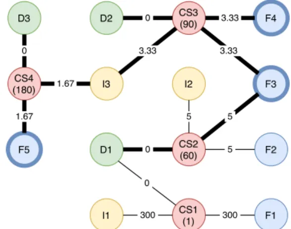
Figure1shows a sample traceability graph, where the graph

includes 300 days of the project history, and the numbers in the parentheses are the days that the commits are made. For example, CS3 was committed at the 90thday (i.e. 210 days ago). All the edges of CS3 have the same distance, which is calculated as follows.

𝐷𝑖𝑠𝑡 𝑎𝑛𝑐𝑒= 1 𝑅𝑒𝑐𝑒𝑛𝑐𝑦 = 1 1−210 300 = 1 0.30 = 3.33

3.2

Jacks (RQ 1.1)

To find Jacks in a software project, we analyze the general knowl-edge of the developers on the project. By looking at the history of the project from its version control data, we can say that the source files keep the knowledge, in other words, the know-how of the project. There are studies to find the authors of source files (e.g. degree of authorship [14]). Authorship is not only about being

the first author of the file but also about changing the source files in time depending on the recency of the change. In our study, we definereachability similar to this definition. If a developer can reach a file, s/he knows that file. Also, multiple developers can reach the same file at the same time. In the following, we explain how we find reachable files and file coverage for each developer.

3.2.1 Finding Reachable Files: We define reachable files of a de-veloper as the files that are reached by the dede-veloper through the connections in the artifact traceability graph. For example, in Figure

1, D2 node can reach every file node in the graph through change

sets, issues and other developers if there is no distance limit (i.e. a limit for the sum of distances on the edges in the graph). Actually, every developer can reach every file if the graph is connected and there is no distance limit. In that case, every developer would know every file, and we could not distinguish which developers know which source files. Also, assuming that all edges having the same importance might be problematic since some edges represent recent commits and reviews while others represent older ones. Our re-cency and distance definitions are utilized here to distinguish these types of situations. For example, the distance between CS3 and F4 is 3.33 while the distance between CS4 and F5 is 1.67, and there are around three months between the commit times of CS3 and CS4. Therefore, to handle these situations, we define the following rules: (1) We need to set a threshold for distance while reaching from one node to another. For example, D2 cannot reach F5 if the threshold is 5 because 3.33+ 1.67 + 1.67 = 6.67 and 6.67 is beyond the threshold 5.

(2) One developer cannot reach files through other developers because it would transfer reachable files of a developer to another developer if the distance threshold is large enough. For example, in Figure1, D2 cannot reach F1 through D1,

even if the distance threshold 308.33 or more.

Distance threshold is a parameter, and it depends on the distance formula given in Equation (2). Due to its nature, distance goes to

infinity when recency goes to zero. In the graph, the oldest relations are the relations from the first day, and their edges have the highest distance. In this case, their distance is calculated as follows:

CS2 (60) F2 I2 D1  0  F3 D2 CS3 (90) F4 I3 CS4 (180) D3 F5  5   5   5   3.33    3.33   0   3.33   1.67   1.67   0  CS1 (1)  0  F1  300  I1  300 

Figure 1: Sample artifact traceability graph. Some nodes and edges are highlighted to illustrate how the reachable files by D2 are found. (D: Developer, F: File, CS: Change Set, I: Issue)

𝐷𝑖𝑠𝑡 𝑎𝑛𝑐𝑒= 1 𝑅𝑒𝑐𝑒𝑛𝑐𝑦 = 1 1−299 300 = 1₁ 300 = 300

Therefore, we need to set our threshold to 300 if we want to use every direct relation in the graph. Since almost all recently changed files are reachable by the developers who have recent commits in that case, using 300 as threshold would not enable us to distinguish which developers know which files.

We follow a simple way while deciding the distance threshold. In a 300-day graph, the edges with 0.1 or less recency belong to the change sets committed in the first 30 days. The rest of the graph corresponds to 90% of the time covered in the graph. Therefore, we can set the distance threshold to 10, which allows us to use all direct relations from the last 90% of the days in the graph. Also, if we set it to 5, 80% of the time would be covered. After this point, we continue with 10 as the distance threshold unless otherwise stated.

𝐷𝑖𝑠𝑡 𝑎𝑛𝑐𝑒= 1 𝑅𝑒𝑐𝑒𝑛𝑐𝑦 = 1 1−270 300 = ₃₀1 300 = 1 0.1 = 10 Figure1shows how reachable files for D2 are found in the sample

graph. The highlighted files (F3, F4, F5) are reachable by D2. While finding these reachable files, we run a depth first search (DFS) algorithm starting from D2 with a stopping condition for reaching the distance threshold. The highlighted edges show the visited edges when DFS is started from D2 node. Also, the DFS algorithm does not go through another developer node. For example, the algorithm stopped when it encountered with the node of D1. Algorithm1

shows the pseudo code for finding reachable files for each developer.

3.2.2 Identifying Jacks: While finding jacks, we sort the developers in descending order according to their file coverage in the software project.File coverage is simply the ratio of the number reachable files by the developer to the number of all files in the project, not just currently available files in the graph. Equation3shows the file

coverage of some developer 𝑑 .

𝐹 𝑖𝑙 𝑒 𝐶𝑜 𝑣 𝑒𝑟 𝑎𝑔𝑒_𝑑=

# of reachable files by 𝑑 # of all files in the project

Algorithm 1 Finding Reachable Files 1: function DevToFiles(𝑔𝑟𝑎𝑝ℎ, 𝑡ℎ𝑟𝑒𝑠ℎ𝑜𝑙𝑑) 2: 𝑑𝑒 𝑣𝑠← 𝐺𝑒𝑡𝐷𝑒𝑣𝑒𝑙𝑜𝑝𝑒𝑟𝑠 (𝑔𝑟𝑎𝑝ℎ) ⊲ list 3: 𝑑𝑒 𝑣𝑇 𝑜 𝑅𝑒𝑎𝑐ℎ𝑎𝑏𝑙 𝑒 𝐹 𝑖𝑙 𝑒𝑠← 𝐻𝑎𝑠ℎ𝑀𝑎𝑝 () ⊲ string to list 4: for 𝑑𝑒𝑣 in 𝑑𝑒𝑣𝑠 do 5: 𝑟 𝑒𝑎𝑐ℎ𝑎𝑏𝑙 𝑒 𝐹 𝑖𝑙 𝑒𝑠← 𝐷𝐹 𝑆 (𝑔𝑟𝑎𝑝ℎ, 𝑑𝑒𝑣, 𝑡ℎ𝑟𝑒𝑠ℎ𝑜𝑙𝑑) 6: 𝑑𝑒 𝑣𝑇 𝑜 𝑅𝑒𝑎𝑐ℎ𝑎𝑏𝑙 𝑒 𝐹 𝑖𝑙 𝑒𝑠 .𝑝𝑢𝑡(𝑑𝑒𝑣, 𝑟𝑒𝑎𝑐ℎ𝑎𝑏𝑙𝑒𝐹𝑖𝑙𝑒𝑠) 7: return 𝑑𝑒𝑣𝑇 𝑜𝑅𝑒𝑎𝑐ℎ𝑎𝑏𝑙𝑒𝐹𝑖𝑙𝑒𝑠

Algorithm 2 Finding Jacks 1: function FindJacks(𝑔𝑟𝑎𝑝ℎ) 2: 𝑑𝑒 𝑣𝑇 𝑜 𝐹 𝑖𝑙 𝑒𝑠← 𝐷𝑒𝑣𝑇 𝑜𝐹𝑖𝑙𝑒𝑠 (𝑔𝑟𝑎𝑝ℎ, 𝑡ℎ𝑟𝑒𝑠ℎ𝑜𝑙𝑑) 3: 𝑑𝑒 𝑣𝑇 𝑜 𝐹 𝑖𝑙 𝑒𝐶𝑜 𝑣 𝑒𝑟 𝑎𝑔𝑒← 𝐻𝑎𝑠ℎ𝑀𝑎𝑝 () ⊲ string to float 4: 𝑛𝑢𝑚𝐹 𝑖𝑙 𝑒𝑠← 𝐺𝑒𝑡 𝑁𝑢𝑚𝐹𝑖𝑙𝑒𝑠 (𝑔𝑟𝑎𝑝ℎ) 5: for 𝑑𝑒𝑣 in 𝑑𝑒𝑣𝑇 𝑜𝐹𝑖𝑙𝑒𝑠.𝑘𝑒𝑦𝑠 () do 6: 𝑛𝑢𝑚𝐷𝑒 𝑣 𝐹 𝑖𝑙 𝑒𝑠 ← 𝑑𝑒𝑣𝑇 𝑜𝐹𝑖𝑙𝑒𝑠 .𝑔𝑒𝑡 (𝑑𝑒𝑣).𝑙𝑒𝑛𝑔𝑡ℎ() 7: 𝑓 𝑖𝑙 𝑒𝐶𝑜 𝑣 𝑒𝑟 𝑎𝑔𝑒←𝑛𝑢𝑚𝐷𝑒 𝑣𝐹 𝑖𝑙 𝑒𝑠 𝑛𝑢𝑚𝐹 𝑖𝑙 𝑒𝑠 8: 𝑑𝑒 𝑣𝑇 𝑜𝐶𝑜 𝑣 𝑒𝑟 𝑎𝑔𝑒 .𝑝𝑢𝑡(𝑑𝑒𝑣, 𝑓 𝑖𝑙𝑒𝐶𝑜𝑣𝑒𝑟𝑎𝑔𝑒) 9: return 𝑆𝑜𝑟𝑡𝐵𝑦𝑉 𝑎𝑙𝑢𝑒 (𝑑𝑒𝑣𝑇𝑜𝐶𝑜𝑣𝑒𝑟𝑎𝑔𝑒)

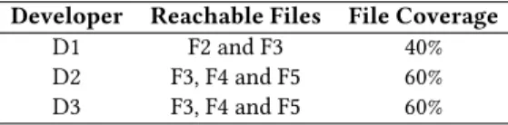
Table 1: Reachable files and file coverages for each developer in the sample artifact traceability graph

Developer Reachable Files File Coverage

D1 F2 and F3 40%

D2 F3, F4 and F5 60%

D3 F3, F4 and F5 60%

Table1shows the reachable files and file coverages for each

developer in the sample artifact traceability graph given in Figure1.

Algorithm2shows the pseudo code of finding jacks. First, it finds

reachable files for each developer, then calculates file coverage scores for developers. Finally, it returns developers in descending order according to their file coverage scores.

3.3

Mavens (RQ 1.2)

By definition, mavens are the rare experts of specific parts, files or modules of the project. As we stated in Section3.2, the source

files in a software project are the reflection of the knowledge (i.e. know-how). Since mavens are the rare expert developers on specific parts, they have knowledge that the others do not have. Thus, we need to find lesser-known parts of the project.

3.3.1 Rarely Reached Files: First, reaching a file through the edges in the artifact graph means knowing the file. To meet the maven definition, we can use the files only reached by a limited number of developers. We call this type of filesrarely reached files, and we set this limit to 1, which means that the files reached by only one developer are therarely reached files. This could be a configurable parameter according to the size of the project. For example, for the graph given in Figure1, F2 is ararely reached file. Actually it is the only one as it can be seen in Table1.

Algorithm3shows how to find rarely reached files. It is assumed

that 𝑑𝑒𝑣𝑇 𝑜 𝑅𝑎𝑟 𝑒 𝐹 𝑖𝑙 𝑒𝑠 is initialized with developer names and empty

Algorithm 3 Finding Rarely Reached Files 1: function DevToRareFiles(𝑔𝑟𝑎𝑝ℎ, 𝑡ℎ𝑟𝑒𝑠ℎ𝑜𝑙𝑑) 2: 𝑑𝑒 𝑣𝑇 𝑜 𝐹 𝑖𝑙 𝑒𝑠← 𝐷𝑒𝑣𝑇 𝑜𝐹𝑖𝑙𝑒𝑠 (𝑔𝑟𝑎𝑝ℎ, 𝑡ℎ𝑟𝑒𝑠ℎ𝑜𝑙𝑑) 3: 𝑓 𝑖𝑙 𝑒𝑇 𝑜 𝐷𝑒 𝑣𝑠← 𝐼𝑛𝑣𝑒𝑟𝑡𝑀𝑎𝑝𝑝𝑖𝑛𝑔(𝑑𝑒𝑣𝑇 𝑜𝐹𝑖𝑙𝑒𝑠) 4: 𝑑𝑒 𝑣𝑇 𝑜 𝑅𝑎𝑟 𝑒 𝐹 𝑖𝑙 𝑒𝑠← 𝐻𝑎𝑠ℎ𝑀𝑎𝑝 () ⊲ string to list 5: for 𝑓 𝑖𝑙𝑒 in 𝑓 𝑖𝑙𝑒𝑇 𝑜𝐷𝑒𝑣𝑠.𝑘𝑒𝑦𝑠 () do 6: 𝑑𝑒 𝑣𝑠← 𝑓 𝑖𝑙𝑒𝑇 𝑜𝐷𝑒𝑣𝑠 .𝑔𝑒𝑡 ( 𝑓 𝑖𝑙𝑒) 7: if devs.length() is 1 then 8: 𝑑𝑒 𝑣𝑇 𝑜 𝑅𝑎𝑟 𝑒 𝐹 𝑖𝑙 𝑒𝑠 .𝑔𝑒𝑡(𝑑𝑒𝑣𝑠 .𝑔𝑒𝑡 (0)).𝑎𝑝𝑝𝑒𝑛𝑑 ( 𝑓 𝑖𝑙𝑒) 9: return 𝑑𝑒𝑣𝑇 𝑜𝑅𝑎𝑟𝑒𝐹𝑖𝑙𝑒𝑠

Algorithm 4 Finding Mavens

1: function FindMavens(𝑔𝑟𝑎𝑝ℎ, 𝑡ℎ𝑟𝑒𝑠ℎ𝑜𝑙𝑑) 2: 𝑑𝑒 𝑣𝑇 𝑜 𝑅𝑎𝑟 𝑒 𝐹 𝑖𝑙 𝑒𝑠← 𝐷𝑒𝑣𝑇 𝑜𝑅𝑎𝑟𝑒𝐹𝑖𝑙𝑒𝑠 (𝑔𝑟𝑎𝑝ℎ, 𝑡ℎ𝑟𝑒𝑠ℎ𝑜𝑙𝑑) 3: 𝑑𝑒 𝑣𝑇 𝑜 𝑀 𝑎𝑣 𝑒𝑛𝑛𝑒𝑠𝑠← 𝐻𝑎𝑠ℎ𝑀𝑎𝑝 () ⊲ string to float 4: 𝑛𝑢𝑚𝑅𝑎𝑟 𝑒 𝐹 𝑖𝑙 𝑒𝑠← 𝐺𝑒𝑡 𝑁𝑢𝑚𝑅𝑎𝑟𝑒𝐹𝑖𝑙𝑒𝑠 (𝑔𝑟𝑎𝑝ℎ) 5: for 𝑑𝑒𝑣 in 𝑑𝑒𝑣𝑇 𝑜𝑅𝑎𝑟𝑒𝐹𝑖𝑙𝑒𝑠.𝑘𝑒𝑦𝑠 () do 6: 𝑛𝑢𝑚𝐷𝑒 𝑣 𝐹 𝑖𝑙 𝑒𝑠← 𝑑𝑒𝑣𝑇 𝑜𝑅𝑎𝑟𝑒𝐹𝑖𝑙𝑒𝑠 .𝑔𝑒𝑡 (𝑑𝑒𝑣).𝑙𝑒𝑛𝑔𝑡ℎ() 7: 𝑚𝑎𝑣 𝑒𝑛𝑛𝑒𝑠𝑠← 𝑛𝑢𝑚𝐷𝑒 𝑣 𝐹 𝑖𝑙 𝑒𝑠 𝑛𝑢𝑚𝑅𝑎𝑟 𝑒 𝐹 𝑖𝑙 𝑒𝑠 8: 𝑑𝑒 𝑣𝑇 𝑜 𝑀 𝑎𝑣 𝑒𝑛𝑛𝑒𝑠𝑠 .𝑝𝑢𝑡(𝑑𝑒𝑣, 𝑚𝑎𝑣𝑒𝑛𝑛𝑒𝑠𝑠) 9: return 𝑆𝑜𝑟𝑡𝐵𝑦𝑉 𝑎𝑙𝑢𝑒 (𝑑𝑒𝑣𝑇 𝑜𝑀𝑎𝑣𝑒𝑛𝑛𝑒𝑠𝑠)

lists. Also, 𝐼 𝑛𝑣 𝑒𝑟 𝑡 𝑀 𝑎𝑝 𝑝𝑖𝑛𝑔 function generate a mapping from val-ues to keys. For instance, it inverts the hashmap{𝐷1 : [𝐹 1], 𝐷2 : [𝐹 1, 𝐹 2]} to the hashmap {𝐹 1 : [𝐷1, 𝐷2], 𝐹 2 : [𝐷2]}.

3.3.2 Identifying Mavens: To find mavens, we consider the number of the rarely reached files of the developers. For a better comparison among developers, we define mavenness of a developer 𝑑 as follows:

𝑀 𝑎𝑣 𝑒𝑛𝑛𝑒𝑠𝑠_𝑑=

# of rarely reached files of 𝑑 # of all rarely reached files

(4)

While finding mavens, first we find reachable files as explained in Section3.2.1, then we find rarely reached files as explained in

Sec-tion3.3.1and given in Algorithm3, finally we calculate mavenness

scores and sort the developers according to them in descending order. Algorithm4shows the procedure.

3.4

Connectors (RQ 1.3)

Connectors are the developers who are involved in different sub-projects or teams. The main idea behind the connector definition is connecting developers who have no other connections, in other words, being the bridge between different groups of developers. Using node centrality, we identify this type of developers on artifact traceability graphs defined in Section3.1.

3.4.1 Calculating Betweenness Centrality: Betweenness centrality of a node is based on the number of shortest paths passing through that node. Freeman [13] discussed that betweenness centrality is

related to control of communication. Also, Bird et al. [5] used

be-tweenness centrality to find the gatekeepers in the social networks of mail correspondents. Therefore, we hypothesize that between-ness centrality can be a measure to find connectors. Betweenbetween-ness centrality of some node 𝑣 where 𝑉 is the set of nodes, 𝑠 and 𝑡 are some nodes other than 𝑣 :

𝑐_𝐵(𝑣) = Õ

𝑠≠𝑣≠𝑡𝜖𝑉

# of shortest paths passing throughv # of shortest (s,t)-paths

(5)

For a better comparison among developers, betweenness values are normalized with 2/( (𝑛 − 1) (𝑛 − 2)) where 𝑛 is the number nodes in the graph. For betweenness centrality related operations, we use NetworkX package2, which uses faster betweenness centrality algorithm of Brandes [6].

To use betweenness centrality, we need a graph composed of only developers because we are looking for developers who connect other developers to each other. Sulun et al.[26] proposed a metric, know-about, to find how much developers know the files. They found different paths between the files and the developers in the artifact graph, and definedknow-about as the summation of the reciprocals of the path lengths. Similarly, we propose to use different paths between developers to find how much they are connected in the artifact graph. The next section explains the details.

3.4.2 Constructing the Developer Graph: Developer graph is a pro-jection of the artifact traceability graph. It defines distances directly between developers in a different way, not as we mentioned in Section3.1. When projecting an artifact graph to a developer graph,

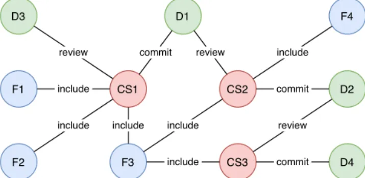
we find all different paths between each developer pair with a depth limit of 4. Since connector definition is not about knowing the files but about connecting the other developers, recency is not a concern and it is assumed that all edges in the artifact graph have the same distance of 1. Thus, depth limit 4 means that the maximum path length can be 4. Therefore, in the traceability graph, two developers can be connected through the paths with length of 2 (through a change set node), or the paths with length of 4 (through 2 differ-entchange set nodes and a file node connected to them). These kinds of paths can be seen in the sample graph in Figure2. We find

the paths between two developers through software artifacts, not through other developers. For example, in Figure2, there is a path

between D2 and D3 through D1, but we interpret this path as the combination of two paths: D1-D2 and D1-D3. Since the develop-ers in the same team potentially work on the same group of files and these files will be close to each other (they will be connected through change sets because they will be changed by the same group frequently) in the traceability graph, the method mentioned above finds the paths between the developers in the same group. So, the developers who have connections in different groups will be favored in betweenness centrality calculations.

After finding the paths between each developer pair, we define a new distance metric, Reciprocal of Sum of Reciprocal Distances (RSRD). We define RSRD as follows when 𝐷 denotes the set of all distances between two developers (i.e. the set of lengths of all different paths between two developers) and 𝑑 is a distance in 𝐷 :

𝑅𝑆 𝑅𝐷= h Õ 𝑑 𝜖 𝐷 𝑑−1 i−1 (6)

Reciprocals of distances make larger contributions to the score for closer nodes. For example,1

2 > 1

4and the path with length of 2 make a larger contribution. After summing the contributions of

2 https://networkx.github.io/ D1 D2 D4 D3 CS2 CS3 CS1 F3 F2 F1 F4  include   include   include   include   include   include   commit   commit   commit  review review review

Figure 2: Another sample artifact traceability graph. (D: De-veloper, F: File, CS: Change Set)

D1 D2 D4 D3 D1 D2 D4 D3 RSRD 2,4,4,4 4,4,4 4,4,4 4 2,4 2,4 0.8 1.33 1.33 1.33 1.33

Figure 3: Sample developer graph. (D: Developer)

all reciprocal distances, larger values represent a stronger connec-tion. For example, the first one means a stronger connection when the first one is 1

2 + 1 4 =

3

4 and the second one is 1 4 + 1 4 = 2 4. To use betweenness centrality, we need to inverse the result of this summation, because the nodes with stronger connections need to be closer. For example, for the numbers in the previous example,

4

3= 1.33 is smaller than 4

2 = 2, and it means a closer relation. At the end, a smaller RSRD score represents a closer relationship between two developers, just like any other distance metric.

Figure3shows how the developer graph is constructed from the

sample artifact graph in Figure2. For example, (2, 4, 4, 4) are the

distances of the different paths between D1 and D2 in Figure2, and

the RSRD between these two developers is calculated as follows:

(2−1+ 4−1+ 4−1+ 4−1)−1=h 1 2+ 1 4+ 1 4+ 1 4 i−1 =h 5 4 i−1 = 0.8 Algorithm5shows the pseudo code for calculating RSRD for a

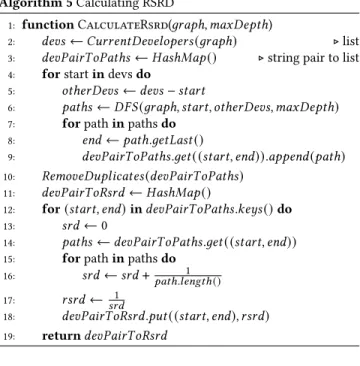
given graph and depth limit. First, it runs a DFS algorithm starting from each developer to find the paths to other developers. Second, it removes duplicates because the DFS results include paths for two ways. For example, DFS finds paths for both(𝐷1, 𝐷2) and (𝐷2, 𝐷1), and it removes(𝐷2, 𝐷1). Then, for each developer pair, it calculates their RSRD value by using the length of the paths.

3.4.3 Identifying Connectors: When identifying connectors, we use the betweenness centrality of developers in the developer graph. Algorithm6shows the procedure. First, it finds different paths and

RSRD values for each developer pair as mentioned above. Then, it creates a developer graph with these RSRD values and finds betweenness centrality for each developer in that graph. Finally, it sorts developers in descending order according to their centrality.

Algorithm 5 Calculating RSRD

1: function CalculateRsrd(𝑔𝑟𝑎𝑝ℎ, 𝑚𝑎𝑥𝐷𝑒𝑝𝑡ℎ)

2: 𝑑𝑒 𝑣𝑠← 𝐶𝑢𝑟𝑟𝑒𝑛𝑡𝐷𝑒𝑣𝑒𝑙𝑜𝑝𝑒𝑟𝑠 (𝑔𝑟𝑎𝑝ℎ) ⊲ list

3: 𝑑𝑒 𝑣 𝑃 𝑎𝑖𝑟𝑇 𝑜 𝑃 𝑎𝑡 ℎ𝑠← 𝐻𝑎𝑠ℎ𝑀𝑎𝑝 () ⊲ string pair to list 4: for start in devs do

5: 𝑜𝑡 ℎ𝑒𝑟 𝐷𝑒 𝑣𝑠← 𝑑𝑒𝑣𝑠 − 𝑠𝑡𝑎𝑟𝑡

6: 𝑝𝑎𝑡 ℎ𝑠← 𝐷𝐹 𝑆 (𝑔𝑟𝑎𝑝ℎ, 𝑠𝑡𝑎𝑟𝑡, 𝑜𝑡ℎ𝑒𝑟 𝐷𝑒𝑣𝑠, 𝑚𝑎𝑥𝐷𝑒𝑝𝑡ℎ)

7: for path in paths do

8: 𝑒𝑛𝑑← 𝑝𝑎𝑡ℎ.𝑔𝑒𝑡𝐿𝑎𝑠𝑡 () 9: 𝑑𝑒 𝑣 𝑃 𝑎𝑖𝑟𝑇 𝑜 𝑃 𝑎𝑡 ℎ𝑠 .𝑔𝑒𝑡( (𝑠𝑡𝑎𝑟𝑡, 𝑒𝑛𝑑)).𝑎𝑝𝑝𝑒𝑛𝑑 (𝑝𝑎𝑡ℎ) 10: 𝑅𝑒𝑚𝑜 𝑣 𝑒 𝐷𝑢𝑝𝑙 𝑖𝑐𝑎𝑡 𝑒𝑠(𝑑𝑒𝑣𝑃𝑎𝑖𝑟𝑇 𝑜𝑃𝑎𝑡ℎ𝑠) 11: 𝑑𝑒 𝑣 𝑃 𝑎𝑖𝑟𝑇 𝑜 𝑅𝑠𝑟 𝑑← 𝐻𝑎𝑠ℎ𝑀𝑎𝑝 () 12: for (𝑠𝑡𝑎𝑟𝑡, 𝑒𝑛𝑑) in 𝑑𝑒𝑣𝑃𝑎𝑖𝑟𝑇 𝑜𝑃𝑎𝑡ℎ𝑠.𝑘𝑒𝑦𝑠 () do 13: 𝑠𝑟 𝑑← 0 14: 𝑝𝑎𝑡 ℎ𝑠← 𝑑𝑒𝑣𝑃𝑎𝑖𝑟𝑇 𝑜𝑃𝑎𝑡ℎ𝑠 .𝑔𝑒𝑡 ( (𝑠𝑡𝑎𝑟𝑡, 𝑒𝑛𝑑))

15: for path in paths do

16: 𝑠𝑟 𝑑← 𝑠𝑟𝑑 + 1 𝑝𝑎𝑡 ℎ .𝑙 𝑒𝑛𝑔𝑡 ℎ() 17: 𝑟 𝑠𝑟 𝑑← 1 𝑠𝑟 𝑑 18: 𝑑𝑒 𝑣 𝑃 𝑎𝑖𝑟𝑇 𝑜 𝑅𝑠𝑟 𝑑 .𝑝𝑢𝑡( (𝑠𝑡𝑎𝑟𝑡, 𝑒𝑛𝑑), 𝑟𝑠𝑟𝑑) 19: return 𝑑𝑒𝑣𝑃𝑎𝑖𝑟𝑇 𝑜𝑅𝑠𝑟𝑑

Algorithm 6 Finding Connectors

1: function FindConnectors(𝑔𝑟𝑎𝑝ℎ) 2: 𝑑𝑒 𝑣 𝑃 𝑎𝑖𝑟𝑇 𝑜 𝑅𝑠𝑟 𝑑← 𝐶𝑎𝑙𝑐𝑢𝑙𝑎𝑡𝑒𝑅𝑠𝑟𝑑 (𝑔𝑟𝑎𝑝ℎ) 3: 𝑑𝑒 𝑣𝐺 𝑟 𝑎𝑝ℎ← 𝐷𝑒𝑣𝑒𝑙𝑜𝑝𝑒𝑟𝐺𝑟𝑎𝑝ℎ(𝑑𝑒𝑣𝑃𝑎𝑖𝑟𝑇 𝑜𝑅𝑠𝑟𝑑) 4: 𝑑𝑒 𝑣𝑇 𝑜 𝐵𝑡 𝑤 𝑛← 𝐵𝑒𝑡𝑤𝑒𝑒𝑛𝑛𝑒𝑠𝑠𝐶𝑒𝑛𝑡𝑟𝑎𝑙𝑖𝑡𝑦 (𝑑𝑒𝑣𝐺𝑟𝑎𝑝ℎ) 5: return 𝑆𝑜𝑟𝑡𝐵𝑦𝑉 𝑎𝑙𝑢𝑒 (𝑑𝑒𝑣𝑇 𝑜𝐵𝑡𝑤𝑛)

4

DATASET

4.1

Selecting Datasets

As we mentioned before, we use software artifacts from project history to construct the artifact traceability graph. More specifically, our approach needs change sets (i.e. commits) and their related data such as author, changed files and linked issues. Rath and Mader [21]

published datasets for 33 OSS projects, SEOSS 33. All 33 datasets are available online3. Out of 33 projects, we selected Apache Hadoop4, Apache Hive5and Apache Pig6since these three projects have the highest issue and change set link ratios among SEOSS 33 datasets. The datasets include data from version control systems (e.g. Git) and issue tracking systems (e.g. Jira). Table2shows the details for

each dataset with a varying number of issues and change sets.

4.2

Preprocessing

Data is already extracted from the version control and issue track-ing platforms and provided in an SQL dataset. Nonetheless, we processed the data in order to prevent errors and calculate specific fields. We did not use all information in the dataset;change_set, code_change and change_set_link tables were enough to create nodes for developers, changes sets, issues and files.

3 https://bit.ly/2wukCHc 4 https://hadoop.apache.org/ 5 https://hive.apache.org/ 6 https://pig.apache.org/

We processed change sets fromchange_set table ordered by commit_date, extracted the data required and dumped them into a file as JSON formatted string of change sets in the temporal order. For each change set, we extracted the following information: commit hash, author, date (commit_date), issues linked, set of file paths with their change types, number of files in the project (after the change set).

In the data extraction, the following points are important: • We only extracted the code changes in java files which, we

assumed, end with ".java" extension. If a change set has no code change including a java file, we ignored it completely. • We ignored merge change sets (is_merge is 1) since they

could inflate the contributions of some developers [1]. • We created a look-up table for each project to detect different

author names of the same authors. They are created manually by looking at the developer names and their email addresses. For example, "John Doe" and "Doe John" can be the same developer if they share a common email address. We used this table to correct the author names by replacing them. • In order to calculate mavenness score (See Section3.3), we

needed the number of files in the project after each change set. Thus, we tracked the set of current files over time. After each code change, we removed the file if its change type is DELETE, and we added the file if its change type is ADD. • Git does not track RENAME situations explicitly, and the

dataset [21] did not share such information about the code

changes. When a file is renamed, it is aDELETE and an ADD for Git (if there is no change in the file)7. In thecode_change table, there are threechange_types: ADD, DELETE and MOD-IFY. In that case, we needed to handle renames because it would affect our traceability graph and change the knowl-edge balance among developers. We treated (DELETE, ADD) pairs in the same change set (commit) asRENAME when the following conditions were satisfied:

– Both have the same file name (file paths are different). – The number of lines deleted in DELETE code change and

the number of lines added inADD code change are equal. So, our rename algorithm only detects file path changes and does not check file contents. For example, it detects RENAME when "example.java" moved from "module1/example.java" to "module2/example.java" but does not detect it when the file content is changed. Since we used the datasets from SQL tables [21] directly and we did not mine them from Git

repositories ourselves, we used the heuristic give. above. • In Hadoop dataset, we detected that there were duplicate

commits. Even though the commit hashes were different, the rest of the extracted data were identical. This situation only applies for Hadoop, the same preprocessing steps did not produce such a situation for Hive and Pig. We removed these change sets by using string comparison for all parts of the JSON string except thecommit hash.

Table2show the number of change sets for each dataset after

preprocessing. Also, we share our implementation online8, and it includes the preprocessing script.

7

https://git-scm.com/book/en/v2/Git-Basics-Recording-Changes-to-the-Repository

8

Table 2: Dataset Details

Project Before Preprocessing [21] After Preprocessing

Time Period (months) # of Issues # of Change Sets Linked Change Sets to a Set of Issues (%) # of Change Sets # of Change Sets added or modified files more than 10

# of Change Sets added or modified files more than 50

Hadoop 150 39,086 27,776 97.13 15178 1900 (12.5%) 129 (0.8%)

Hive 113 18,025 11,179 96.34 9030 1062 (11.8%) 127 (1.4%)

Pig 123 5234 3134 92.85 2401 240 (10.0%) 32 (1.3%)

4.3

Handling Large Change Sets

Change set means a set of file changes, and it is called large change set when the number of changed files is more than a specific number. For example, initial commits of a project most probably include many files, and it is a typical example for large commits. Another example is moving a project into another project. In that case, its change set includes all the files in the added project.

Committing a large number of files in one change set is not considered to be a good practice in software engineering. Sadowski et al.[25] claim that 90% of the changes in Google modify less than

10 files. Also, Rigby and Bird [22] excluded the changes that contain

more than 10 files in their case studies. In our experiments, we use a looser limit for excluding change sets. In the following, we explain the details on removing the large change sets:

• Regardless of the size of a change set, we apply changes to the traceability graph forDELETE and RENAME types. Since the knowledge of deleted files is not required after that point and renamed files need to proceed with their new names. • If a change set includes more than 50 files which are added or

modified, we ignore theseADD and MODIFY code changes. We did not use 10 as the limit because we did not want to lose 10.0-12.5% of the datasets (See Table2). Also, sometimes

large commits can exist even though it is not a good practice. Our purpose is handling initial commits of the projects and project movements. So, choosing 50 is a good trade-off for the limit of the number of files added or modified in a change set. It is not that small to cause losing 10.0-12.5% of the datasets and not that large to include commits like initial commits.

5

CASE STUDIES

5.1

Experimental Setup

In the experiments, we used NetworkX package2for graph op-erations. In order to prevent potential bugs, we used its built-in functions whenever possible (e.g. calculating betweenness central-ity, finding paths between developers). However, we implemented the DFS algorithm for reachable files in Algorithm1because it was

very specific to our case (e.g. the stopping condition is different). Our source code is available online8.

How much time the artifact graph should cover is a parame-ter in our method. We chose a sliding window approach over an incremental window in time, in other words, the artifact graph al-ways includes the change sets committed in a constant time period. Followings are the reasons behind this choice:

• If the time period of the graph changes over time, the mean-ing of the recency changes. For example, 0.9 recency means

1 2 3 ... 365 366 367 368 369 ... 1 2 3 ... 365 366 367 368 369 ... 1 2 3 ... 365 366 367 368 369 ... Step 1 Last Step Step 2 3367 3001 3002 3003 ... 3365 3366  TIMELINE (days)  1 year (365 days) 3367 3001 3002 3003 ... 3365 3366 3367 3001 3002 3003 ... 3365 3366

Figure 4: Experimental Setup

30 days ago in a 300-day graph while the same recency corre-sponds to 50 days ago in a 500-day graph. Thus, keeping the time period (sliding windows size) constant enables recency scores to have the same meaning in different time points. • Keeping every artifact from history enlarges the graph every

day, and the algorithms run slower in larger graphs. There-fore, removing unnecessary parts (the artifacts older than one year) means less run time.

• In OSS projects, there is no data about leaving developers. If we keep every artifact from the history, we should calculate scores even for former developers. Therefore, removing old artifacts enables us to keep track of the current developers. If the graph keeps the last 365 days, we assume the developers who contributed to the project in the last 365 days are the current active developers.

We used a 1-year (365 days) sliding window in our experiments. Figure4shows how the included days change in iterations. The

numbers on the figure come from the Hive dataset. "3367 days" corresponds to the number of days after preprocessing. There are 3003 iterations including the initial window. We tracked the dates over change sets. When forwarding the window one day, firstly, we removed the change sets of the first day of the window. Then, we added the change sets of the day after the last day of the win-dow. For each iteration, we calculated scores for jacks, mavens and connectors, then, we reported them and their scores in descending order. The same procedure was repeated for Hadoop and Pig.

5.2

Results

Since we propose to usejack, maven and connector as the key developer categories for the first time and there is no classification of developers for these types in the literature, we are not able to compare our approach with others. Also, since we conducted our experiments on OSS projects, we have no data for developer labels for these projects. However, we can show that the results of our approach are compatible with other statistics of the projects.

To validate our approach, we propose to use developers’ com-ments on issues.Jacks are the developers who have broad knowl-edge by definition, and we identified them by finding their file

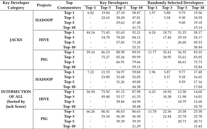
Table 3: Mean accuracy percentages for the key developers of our approach vs. the developers selected randomly in Monte Carlo simulation Key Developer Category Projects Top Commenters

Key Developers Randomly Selected Developers

Top-1 Top-3 Top-5 Top-10 Top-1 Top-3 Top-5 Top-10

JACKS HADOOP Top-1 6.82 19.04 27.10 50.47 1.97 5.88 9.79 19.56 Top-3 - 22.65 30.20 47.81 - 5.58 9.30 18.59 Top-5 - - 29.62 47.40 - - 9.60 19.18 Top-10 - - - 41.75 - - - 19.14 HIVE Top-1 44.16 71.43 81.65 92.21 6.24 18.73 31.23 58.17 Top-3 - 54.78 70.20 84.12 - 17.46 29.10 54.17 Top-5 - - 57.02 73.28 - - 26.60 49.53 Top-10 - - - 55.31 - - - 38.84 PIG Top-1 59.16 86.23 88.90 89.91 11.77 35.41 56.35 83.55 Top-3 - 75.27 85.26 89.99 - 34.95 55.61 83.05 Top-5 - - 66.91 79.66 - - 46.61 73.73 Top-10 - - - 59.15 - - - 55.84 INTERSECTION OF ALL (Sorted by Jack Score) HADOOP Top-1 7.22 21.33 34.97 59.04 1.96 5.87 9.77 17.48 Top-3 - 23.80 32.68 52.05 - 5.57 9.28 16.65 Top-5 - - 31.26 49.08 - - 9.59 17.16 Top-10 - - - 44.38 - - - 17.04 HIVE Top-1 56.94 75.92 81.15 87.98 6.23 10.92 12.50 14.68 Top-3 - 49.40 55.17 61.33 - 10.38 11.90 14.01 Top-5 - - 38.86 44.94 - - 10.79 12.68 Top-10 - - - 30.48 - - - 10.70 PIG Top-1 66.26 86.41 86.63 86.63 11.78 22.36 23.58 23.58 Top-3 - 55.54 56.30 56.30 - 22.44 23.78 23.78 Top-5 - - 39.39 39.39 - - 20.73 20.73 Top-10 - - - 21.29 - - - 15.45

coverage in the project. Therefore, thejacks should be involved in the issues such as bugs and enhancements more than other de-velopers. We claim that, by definition, the topjacks and the top commenters in the project’s issue tracking system (e.g. Jira) should be mostly the same developers. However, we cannot claim that mavens and connectors should be among the top commenters. To validate the results of these categories, we offer to use the develop-ers who arejack, maven and connector at the same time, in other words, the intersection of all kinds of key developers. In that way, we includemavens and connectors to our validation, and we show how the intersection developers overlap with the top commenters. While using the intersection developers, we sorted them by their jack score (i.e. file coverage) since we cannot combine betweenness centrality, mavenness score and file coverage properly. So, in the case studies, we examined the jacks and the intersection developers. The datasets [21] we used for experiments include data from

issue tracking systems (e.g. Jira). In thechange_set_link table, there are links between issues and change sets, which means we can use the comments made to issues in the traceability graph. The datasets supply thedisplay_name of the commenters in issue_comment table. The names in thedisplay_name field matches the developer names inauthor field of change_set table. So, we can find which developers made how many comments to the issues in the graph. To increase the validity of the number of comments for each developer, we corrected the commenter names by using the look-up table created manually in preprocessing (See Section4.2).

TheKey Developers column in Table3shows the accuracy of our approach when we treat the top commenters as the actual key developers (i.e. ground truth). "Top commenters" means a ranked list of commenters according to the number of comments that they made to the issues in the last year. The predicted key developers by our model are consistent with the top commenters up to 92%.

Accuracy is calculated as shown in Equation7, where 𝐾 𝐷 is the

ranked list of key developers, 𝐶 is the ranked list of commenters, 𝐷 is the set of dates (i.e. days or iterations in Figure4) and k refers

the numbers in Top-k phrases in the Table3. For example, the

accuracy of day 𝑑 for (Top-3, Top-5) cell is calculated as follows: If 𝐶 𝑑(3) = {𝐷1, 𝐷2, 𝐷3} and 𝐾𝐷𝑑(5) = {𝐷1, 𝐷2, 𝐷4, 𝐷5, 𝐷6}, the accuracy is | {𝐷1,𝐷2} | | {𝐷1,𝐷2,𝐷3} | = 2 3= 0.67. 𝑀 𝑒𝑎𝑛 𝐴𝑐𝑐𝑢𝑟 𝑎𝑐𝑦(𝑘1, 𝑘2) = 1 |𝐷 | 𝐷 Õ 𝑑 |𝐶𝑑(𝑘1) ∩ 𝐾𝐷𝑑(𝑘2) | |𝐶𝑑(𝑘1) | (7)

Since there is no comparable approach that finds our subcate-gories of key developers, we used the Monte Carlo simulation as a baseline approach. We randomly selected the key developers for each day from the existing developers in the graph, in other words, from the developers who committed changes to the source code in the sliding window period. While producing random developers, we considered the number of key developers in our results since the simulation should provide random results in the same struc-ture. For example, we selected 4 random developers if our approach

found 4 jacks in that day even if 𝑘₂is 5. Then, we calculated mean accuracies in the same way shown in Equation7. This experiment

with random key developers is repeated 1000 times. TheRandomly Selected Developers column in Table3shows the average of the accuracies of 1000 simulations. It can be seen that our approach is more successful than the random model for all cases.

Hadoop, Hive and Pig have different scales. Pig is a small project with tens of developers while the others have hundreds of develop-ers in their whole history. Even though they both have hundreds of developers and their time periods are not that different, Hadoop has a lot more change sets and issues than Hive as shown in Table

2. The average number of active developers for each project, in

other words, the average number of developers in the traceability graph over time are as follows: 9.05 in Pig, 35.08 in Hive and 49.86 in Hadoop. So, it is clear that Hadoop is a more active project than Hive. Also, the differences between the results of projects in Table

3infer the same conclusion. Both the results of our algorithms and

the results of Monte Carlo simulation show that the more active developers exist, the harder it becomes to predict key developers. Even though the accuracies are different among the projects due to the fact mentioned above, our results are better than the results of the random model for all cases. Also, the key developers predicted by our approach and the top commenters overlap up to 92%.

5.3

Discussion

In this section, we discuss the studies which propose a definition for core, hero, key or LTC developers similar to our definition.

Agrawal et al. [1] worked on hero developers in software projects.

According to their definition, a project has hero developers if 20% of the developers made 80% of the contributions. Hero developers are similar to key developers in our case, as projects mostly depends on them. The authors provided a definition for the projects with hero developers, then analysed hero and non-hero projects without providing a validation. In our study, we subcategorized the key developers into three categories and provided separate algorithms to identify key developers.

Oliva et al. [20] worked on characterizing the key developers,

that is "the set of developers who evolve the technical core". First, they detected the commits to core files in the project. Then, they ranked the developers according to their core commit counts, and considered first 25% of the list as key developers. Without validating their key developers, they analyzed the identified key developers in terms of contribution characteristics, communication and coordina-tion within the project. Also, they only performed an experiment on a small project with 16 developers. In our study, we investigated our algorithms in three projects different in size, and validated our key developers using top commenters in issue tracking systems.

Crowston et al. [10] examined the core and periphery of OSS

team communications. They analyzed if the three following meth-ods produce similar results or not: the contributors named officially (e.g. support manager, developer), the contributors who contribute the most to the bug reports, and the contributors who are defined by a pattern of interactions in bug tracking systems. Since they used data from SourceForge9, they had access to official labels of the contributors. In our case, Git repositories does not provide any

9

https://sourceforge.net/

labels for developer roles in the project and Apache organization only provide the full list of current developers.

Joblin et al.[16] studied core and peripheral developers. The core

developers are the essential developers in the projects as the key developers in our study. They worked on count-based (e.g. number of commits as in [1]) and network-based (e.g. degree centrality in

developer graph from version control systems and mailing lists) metrics. They established a ground truth by making a survey with 166 participants. We were not able to examine their data because the project and survey data links are not accessible through their website10. Also, their survey shows the actual core developers for a snapshot of the time, while our approach provide results continu-ously with a sliding window approach.

Zhou and Mockus [28] defined an LTC as "a participant who

stays with the project for at least three years and is productive". They claimed that LTCs are crucial for success of the projects. They mainly investigated how a new joiner become an LTC (i.e. a valuable contributor). In our study, we investigated how to find key developers rather than examining how new joiners evolve in time.

6

THREATS TO VALIDITY

Construct validity is about how the operational measures in the study represent what is investigated according to the RQs [24]. We

used a dataset from another study[21], and their mining process

can potentially affect our results. To reduce the threat caused by the data mining process, we eliminated the possible problems (e.g. we corrected author names manually by looking at their names and email addresses.) in preprocessing (See Section4.2). However, there

might still be problems related to data integrity.

Internal validity concerns if the causal relations are examined or not [24]. While building the graphs and defining algorithms, we

made many decisions related to thresholds including choosing 50 as the limit for the number of files added or modified in a change set, choosing 10 as the distance threshold in file reachability and using 365-day (1-year) sliding window in the experiments. We tried various options and made the final decisions after evaluating their results. In the corresponding sections of this study, we shared the justifications behind these decisions. For example, we chose 10 as the distance threshold since it corresponds to 90% of the covered time in the graph because of the nature of the distance formula.

The potential errors in the implementation of our approach threaten the validity of our results. We benefited from a stable graph package NetworkX2in our operations and used its methods whenever possible, for example, betweenness centrality calcula-tions and DFS for finding paths between developers. To prevent potential bugs, we performed multiple code review sessions with a third researcher. Also, we shared the implementation online8for replicability of the results.

We used developer comments in issue tracking systems to vali-date our approach, however, we do not claim that the number of comments shows the key developers in a project. We just claim that there should be a correlation between the top commenters and the key developers in the same time period. Then, we used this idea to show that our approach produced more logical results than the random case with a Monte Carlo simulation.

10

External validity concerns about generalization of the find-ings in studies [24]. In our case studies, we used three different

OSS projects. Even though we did not conduct a case study in an industrial company, we selected projects from Apache11, a 20-year established foundation. Also, the sizes of the projects are differ-ent as seen in Table2. Although we believe that we have enough

data for an initial assessment, in the future, we need to run our algorithms in more OSS and industrial datasets.

7

CONCLUSION AND FUTURE WORK

In this study, we proposed different categories for key developers in software development projects:jacks, mavens and connectors. To identify the developers in these subcategories of key developers, we proposed separate algorithms. Then, we conducted case studies on three OSS projects (Hadoop, Hive and Pig). Since there was no labeled data for the key developer categories, we used developers’ comments in issue tracking systems to validate our results. The key developers found by our model were compatible with the top commenters up to 92%. The results indicated that our approach has promising results to identify key developers in software projects. We can summarize the contributions of our study as follows:

• We offered a novel categorization for the key developers inspired by The Tipping Point from Gladwell [15]. • For each of the three key developer categories (jacks, mavens

and connectors), we proposed the corresponding algorithms using a traceability graph (network) of software artifacts. • The findings of this study might shed light on the

truck-factor problem. Key developers can be used to find the truck factor of the projects.

• Identifying key developers in a software project might help the software practitioners for making managerial decisions.

As future work, we plan to run our algorithms on the projects in industrial datasets and validate our results by interviewing project stakeholders and creating a labeled dataset for these types of key developers. We are also planning to use the artifact traceability graph to categorize projects (balanced or hero) and recommend replacements for leaving developers.

REFERENCES

[1] Amritanshu Agrawal, Akond Rahman, Rahul Krishna, Alexander Sobran, and Tim Menzies. 2018. We don’t need another hero?: the impact of heroes on software development. InProceedings of the 40th International Conference on Software Engineering: Software Engineering in Practice. ACM, 245–253.

[2] Mohammad Y Allaho and Wang-Chien Lee. 2013. Analyzing the social ties and structure of contributors in open source software community. In_Proceedings of the 2013 IEEE/ACM International Conference on Advances in Social Networks Analysis and Mining. 56–60.

[3] Guilherme Avelino, Eleni Constantinou, Marco Tulio Valente, and Alexander Serebrenik. 2019. On the abandonment and survival of open source projects: An empirical investigation. In_{2019 ACM/IEEE International Symposium on Empirical} Software Engineering and Measurement (ESEM). IEEE, 1–12.

[4] Guilherme Avelino, Leonardo Passos, Andre Hora, and Marco Tulio Valente. 2016. A novel approach for estimating truck factors. In_{2016 IEEE 24th International} Conference on Program Comprehension (ICPC). IEEE, 1–10.

[5] Christian Bird, Alex Gourley, Prem Devanbu, Michael Gertz, and Anand Swami-nathan. 2006. Mining email social networks. InProceedings of the 2006 interna-tional workshop on Mining software repositories. 137–143.

[6] Ulrik Brandes. 2001. A faster algorithm for betweenness centrality.Journal of mathematical sociology 25, 2 (2001), 163–177.

11

https://www.apache.org/

[7] H Alperen Cetin. 2019. Identifying the most valuable developers using artifact traceability graphs. InProceedings of the 2019 27th ACM Joint Meeting on European Software Engineering Conference and Symposium on the Foundations of Software Engineering. 1196–1198.

[8] Jinghui Cheng and Jin LC Guo. 2019. Activity-based analysis of open source software contributors: roles and dynamics. In_{2019 IEEE/ACM 12th International} Workshop on Cooperative and Human Aspects of Software Engineering (CHASE). IEEE, 11–18.

[9] Valerio Cosentino, Javier Luis Cánovas Izquierdo, and Jordi Cabot. 2015. Assessing the bus factor of Git repositories. In_{2015 IEEE 22nd International Conference on} Software Analysis, Evolution, and Reengineering (SANER). IEEE, 499–503. [10] Kevin Crowston, Kangning Wei, Qing Li, and James Howison. 2006. Core and

periphery in free/libre and open source software team communications. In Pro-ceedings of the 39th Annual Hawaii International Conference on System Sciences (HICSS’06), Vol. 6. IEEE, 118a–118a.

[11] Enrico Di Bella, Alberto Sillitti, and Giancarlo Succi. 2013. A multivariate classi-fication of open source developers.Information Sciences 221 (2013), 72–83. [12] Mívian Ferreira, Thaís Mombach, Marco Tulio Valente, and Kecia Ferreira. 2019.

Algorithms for estimating truck factors: a comparative study.Software Quality Journal 27, 4 (2019), 1583–1617.

[13] Linton C Freeman. 1978. Centrality in social networks conceptual clarification. Social networks 1, 3 (1978), 215–239.

[14] Thomas Fritz, Gail C Murphy, Emerson Murphy-Hill, Jingwen Ou, and Emily Hill. 2014.Degree-of-knowledge: Modeling a developer’s knowledge of code. ACM Transactions on Software Engineering and Methodology (TOSEM) 23, 2 (2014), 1–42.

[15] Malcolm Gladwell. 2006. The tipping point: How little things can make a big difference. Little, Brown.

[16] Mitchell Joblin, Sven Apel, Claus Hunsen, and Wolfgang Mauerer. 2017. Clas-sifying developers into core and peripheral: An empirical study on count and network metrics. In_{2017 IEEE/ACM 39th International Conference on Software} Engineering (ICSE). IEEE, 164–174.

[17] Takeshi Kakimoto, Yasutaka Kamei, Masao Ohira, and Kenichi Matsumoto. 2006. Social network analysis on communications for knowledge collaboration in oss communities. In_{Proceedings of the International Workshop on Supporting} Knowledge Collaboration in Software Development (KCSD’06). Citeseer, 35–41. [18] Makrina Viola Kosti, Robert Feldt, and Lefteris Angelis. 2016. Archetypal

person-alities of software engineers and their work preferences: a new perspective for empirical studies.Empirical Software Engineering 21, 4 (2016), 1509–1532. [19] Audris Mockus. 2010. Organizational volatility and its effects on software

de-fects. InProceedings of the eighteenth ACM SIGSOFT international symposium on Foundations of software engineering. 117–126.

[20] Gustavo Ansaldi Oliva, José Teodoro da Silva, Marco Aurélio Gerosa, Francisco Werther Silva Santana, Cláudia Maria Lima Werner, Cleidson Ronald Botelho de Souza, and Kleverton Carlos Macedo de Oliveira. 2015. Evolving the system’s core: a case study on the identification and characterization of key developers in Apache Ant.Computing and Informatics 34, 3 (2015), 678–724.

[21] Michael Rath and Patrick Mäder. 2019. The SEOSS 33 dataset—Requirements, bug reports, code history, and trace links for entire projects.Data in brief 25 (2019), 104005.

[22] Peter C Rigby and Christian Bird. 2013. Convergent contemporary software peer review practices. In_{Proceedings of the 2013 9th Joint Meeting on Foundations of} Software Engineering. 202–212.

[23] Peter C Rigby, Yue Cai Zhu, Samuel M Donadelli, and Audris Mockus. 2016. Quantifying and mitigating turnover-induced knowledge loss: case studies of Chrome and a project at Avaya. In_{2016 IEEE/ACM 38th International Conference} on Software Engineering (ICSE). IEEE, 1006–1016.

[24] Per Runeson and Martin Höst. 2009. Guidelines for conducting and reporting case study research in software engineering._{Empirical software engineering 14, 2} (2009), 131.

[25] Caitlin Sadowski, Emma Söderberg, Luke Church, Michal Sipko, and Alberto Bacchelli. 2018. Modern code review: a case study at google. InProceedings of the 40th International Conference on Software Engineering: Software Engineering in Practice. 181–190.

[26] Emre Sülün, Eray Tüzün, and Uğur Doğrusöz. 2019. Reviewer Recommenda-tion using Software Artifact Traceability Graphs. InProceedings of the Fifteenth International Conference on Predictive Models and Data Analytics in Software Engineering. 66–75.

[27] Jing Wu and Khim Yong Goh. 2009. Evaluating longitudinal success of open source software projects: A social network perspective. In2009 42nd Hawaii International Conference on System Sciences. IEEE, 1–10.

[28] Minghui Zhou and Audris Mockus. 2012. What make long term contributors: Will-ingness and opportunity in OSS community. In_{2012 34th International Conference} on Software Engineering (ICSE). IEEE, 518–528.