Family of scaling chirp functions, diffraction, and holography

1568 IEFE TRANSACTIONS ON SIGNAL PROCESSING, VOL. 43, NO. 7, JULY 1995

Family of Scaling Chirp Functions,

Diffraction, and Holography

Levent Onural,

Senior Member, ZEEE,

and

Mefharet Kocatepe

Abstruct- It is observed that diffraction is a convolution operation with a chirp kernel whose argument is scaled. F d y of functions obtained from a prototype by shifting and argument

sealing form the essential ground for wavelet framework. There- fore, a connection between diffraction and wavelet transform is

developed. However, wavelet transform is essentially prescribed for time-frequency and/or multiresolution analysis which is ir-

relevant in our case. Instead, the proposed framework is useful in various location-depth type of analysis in imaging. The linear transform when the analyzing functions are the chirps is called

the scaling chirp transform. The scaled chirp functions do not satisfy the commonly used admissibility condition for wavelets. However, it is formally shown that these neither band nor time limited signals can be used as wavelet functions and the inversion

is still possible. Diffraction and in-line holography are revisited within the scaling chirp transform context. It is formally proven that a volume in-line hologram gives perfect reconstruction. The developed framework for wave propagation based phenomena has the potential of advancing both signal processing and optical applications.

I. INTRODUCTION

HE LITERATURE on mathematical analysis and appli-

T

cations of wavelets and wavelet transforms has reached to a significant level over the past years. Tutorial articles [ l ] and [2] give plenty of references. An overview of the basics is also presented in [3] and [4]. It seems like the major motivation in wavelet decomposition is the time-frequency analysis of signals. (see for example, [4], chapter 1) The set of kernels which are obtained from a single function by scaling its argument and by shifting brings a simple structure. Means of selecting a subset of these functions as orthogonal basis vectors yield a convenient multiresolution analysis [ 5 ] . The conditions which are imposed on wavelet functions are consequences of the desire to have proper and useful time-frequency, or multiresolution, analysis. To be more specific, the “admissibility condition” [3] assures invertibility (thus makes the transform useful) and imposes the necessary features, like the zero value of the Fourier transform at the origin, to have a time-frequency (or multiresolution) analysis. Actually, what is done is a time-scale analysis, and the overall structure is developed so that the scale corresponds

Manuscript received November 23,1993; revised November 21,1994. The associate editor coordinating the review of this paper and approving it for publication was Dr. Patrick Flandrin.

L. Onural is with the Electrical and Electronics Engineering Department, Bikent University, Ankara, Turkey.

M. Kocatepe is with the Mathematics Department, Bilkent University,

Ankara, Turkey.

EEE Log Number 9412004.

to frequency to achieve time-frequency analysis to satisfy the primary motivation.

However, there are many other possible applications of scale-and-shift based structures where the main concem is not the time-frequency, nor the multiresolution analysis. In -this paper, we present such a case. We still have a mother kemel which is a chirp function, and obtain daughter kernels from that by shifting and scaling; we find the projections of an arbitrary function onto these kernels by inner products, and we show that the original function can be reconstructed from these inner products. The kemels are called scaling chirp functions and the set of inner products is called scaling chirp transform in this paper. However, our kemels, being chirp

functions, are neither time nor band limited, therefore, violate the admissibility condition; the scale does not correspond to frequency but spatial depth in a wave propagation envi- ronment. Yet the reconstruction formulas have similar forms as the reconstruction formulas of wavelets, even though the admissibility condition is violated.

We are motivated by the observation that the scaling chirp kernels which represent wave propagation in free space have the scaling property of a wavelet family. The scale, in this case, is associated with the distance that a wave propagates. Since the propagation is modeled by convolutions with these kemels, the process of finding the field in 3-D space from a given 2-D cross-section is functionally and algorithmically the same as finding the wavelet transform of the 2-D pattem. Knowing the fundamental wave propagation related phenomena like diffraction and holography, and their mathematical models, we expected that the inversion formulas must exist even though the admissibility condition of [3] is not satisfied; because, the existing optical theory and applications show that these transforms are invertible [6]. Formal proof for the invertibility is given in this paper. The form of the inversion formulas is intentionally made similar to the inversion formulas of the wavelets [3]. If the multiresolution analysis is not of concem, and thus, if the invertibility is sufficient when selecting scal- ing kernels, then these chirp kemels are also admissible as evident from the existence of the inversion formulas. Many related inversion formulas are presented: each one has its own significance in different contexts. Since these functions represent wave propagation in space, the proposed framework is useful for space-depth analysis as opposed to the time- frequency analysis related to wavelets. Space-depth analysis can be directly applied in many wave propagation based data collection and interpretation problems, like the analysis of holographic data [16]. An example is illustrated by Figs. 1 and 1053-587X/95$04.00 0 1995 IEEE

ONURAL AND KOCATEPE: FAMILY OF SCALING CHIRP FUNCTIONS, DIFFRACTION, AND HOLOGRAPHY

I.

1569 $1 I

/ ’

I

location,

x

x

Fig. 1. Simulated 1-D hologram. The horizontal axis is the x-coordinate and the gray value variation is the f ( . r ) . (Dark is low and white is high.) The simulation is carried out as described in [9]. This is an in-line hologram of three rather small I-D objects (thin infinite length wires, for example) whose .r-coordinates are located at the centers of the corresponding three broader dark bands. Each object is located at a different depth. If the original scene, instead of this hologram, were viewed, three thin dark stripes at different locations and depths on an illuminated background would be seen.

2. Fig. 1 shows a simulated 1-D hologram (there is no variation in the vertical direction). This is a simulated hologram of three 1 -D objects concentrated at different :E-coordinates (locations) each having different depths (z-coordinates). If this hologram is used as a diffraction grid, the diffracted wave will focus at different ( T , z ) coordinates, revealing the .z-coordinate (the

location) and the depth of the original I-D objects. Similarly, if the I-D holographic signal is processed by the scaling chirp transform, the concentrations of the signal in space- scale domain will give the locations and depths (i.e., the (x.z) coordinates) of the original three objects. The result of the scaling chirp transform is shown in Fig. 2. Here, the

x-

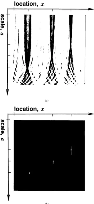
coordinate is the horizontal axis, and the scale is the vertical axis. The scale and physical depth are related to each other by a square-law relation as described later in this paper. The scaling chirp transform has a good performance in localizing signal components in space-scale (depth) domain as seen in Fig. 2.

Some related wavelets have appeared in the literature with the name of “chirplets,” and the associated transforms are called “chirplet transforms” [7]. Essentially, the chirplet func- tions are band and time localized versions of the scaling chirp functions. Each chirplet, with its parameter set, rep- resent a tile of the time-frequency plane. Therefore, these chirplet kemels are also useful for time-frequency analysis applications. The functions considered in this paper are neither time nor bandlimited, and therefore, mathematical properties are significantly different. The intended applications are also different than the time-frequency analysis, as explained above. It is shown with proofs, in this paper, that the diffraction and holography can be put into a scaling kemel framework. After a carefully developed mathematical structure, one-to-one

v) 0

“5

a

v) 0

“5

a

location,

x

I I _{I I I}

-

(a)

location,

x

(b)

Fig. 2. Two figures representing the scaling chirp transform of the hologram of Fig. 1. In both (a) and (b), the horizontal axis is the .c-coordinate, and the vertical coordinate is the scale. The scale parameter o increases from top to bottom. The physical depth 3 is related to the scale parameter CL. The

scaling chirp transform is complex valued. (a) The intensity of the scaling chirp transform of f ( . c ) of Fig. 1. The three dark nodes give the locations of the signal concentrations (i.e.. the dark objects over a bright background) over the (r, a ) space. (b) To have a better visualization, the dc part of the scaling chirp transform is eliminated, and then, its intensity is taken. The three bright dots show the .r-coordinates and the depths of the three original objects,

correspondences between the mathematical results and various practical diffraction and holography related phenomena are pointed out. Possible further uses of these results are discussed in the last section of the paper.

We would like to comment also on the terminology. In the literature, the scale and shift based kernels are almost

1570 IEEE TRANSACTIONS ON SIGNAL. PROCESSING, VOL. 43, NO. 7, JULY 1995 always associated with the wavelets in a time-frequency, or

multiresolution, context. So, it looks like the term “wavelets” is used whenever the shift and scale of a mother kernel is the primary feature, but the other restrictions due to time- frequency nature are also either explicitly stated or implied. Recently, we preferred to use the term “wavelets” also for our case where the shift and scale features are the same as the conventional wavelet approach [ 151. However, in our case, we do not meet the other conventional constraints, because the time-frequency (or multiresolution) analysis is not the issue. The discriminating features of scaling functions and wavelet functions are clear in a multiresolution framework [ 5 ] . However, once the multiresolution analysis (or any tiling of the time-frequency space) is left out, as in our case, the terminology also becomes obscure. As a consequence, we decided to refer the kernels as scaling chirp functions instead

of wavelets, in this paper. We believe that the terminology will also become clarified as applications using shifted and scaled kernels in a context other than time-frequency or multiresolution analysis emerge.

11. THE WAVELET CONCEPT AND DIFFRACTION The principles of diffraction can be found in classical references like Born and Wolf [6]. In 3-D space, the field at a distance z from a planar distribution +(z, y ) is given by the Huygens-Fresnel approximation as [8]

where

With these observations, it is easy to see that the convolution kernels of (2) and (6) have the scale and shift features of a wavelet family for 2- and 1-D function spaces, respectively. Classically, wavelets are a family of functions, obtained from one single function, indexed by two parameters as [3]

(7)

where w is a function which satisfies

C, =

I w I - ~ I W ( W ) ~ ~

dw

<

00. (8)

W ( w ) is the Fourier transform of ~ ( 2 ) . The inner product of a

function

4

with one of the wavelet functions gives a coefficient corresponding to the parameters a and b. Such inner products

for all a’s and b’s constitute a representation for the function

4

as

where the inner product is defined by

(9)

( j t [($ - 6 ) 2 + (y

-

.r)2])dtds (1) The inner product

4)

is a 2-D function of a and b, and this function is called the wavelet transform of

4.

It is easy to see from (1) and (4) that the diffraction kernel is indeed used by shifting and scaling it, as in the wavelet analysis- When the chirp f u n d o n

where A is the wavelength. Here, the phase of the wave is assumed to be increasing as we go away from the source. The constant D may be chosen arbitrarily with the implication of a corresponding reference amplitude and phase. From now on,

the constant

D

will be absorbed into the function $(z, y), so h ( s ) = exp(jx2) (11) it will not appear in the equations. This relationship may be

represented as a linear shift-invariant system with an impulse response [9]

is taken as the mother wavelet, all other daughter functions of the family can be obtained as

where a =

4%

and b = {. The amplitude modifier .(a) can (3) be found as

where t* represents 2-D convolution. _{.(a) = exp ( j}

2

_{2) = e x p [ j ( 2 ( y ) 2}

_-

$)]

J;;..

₁

(13) As a consequence of this definition of the amplitude modifier, in (7) and (12). This is not a difficulty, though. The amplitude scaling as given by (7) is the result of having the total energy

1cIz(x) = -exp

(

j - z

)

J;$(E)eXP(j;(x -

E)’)@.

of the daughter functions the same as the energy of the mother wavelet. Although this is a suitable choice for various applications, this requirement is definitely not strict, and can be violated. However, depending on this amplitude scale, the integrability condition must be derived again. For an amplitude

m

A similar representation may also be given for waves prop- agating in 2-D space. For this case, the 1-D field distribution given as

at a distance from a (line) Source distribution is the amplitude scaling due to the a is different

1

(4)

m

Again, using the linear system notation, we get

ONURAL AND KOCATEPE: FAMILY OF SCALING CHIRP FUNCTIONS, DIFFRACTION, AND HOLOGRAPHY 1571 scaling by la/-' instead of lnl-'/2, the integrability condition

is already derived in [IO]. Any other scaling can be treated in a similar way. A rather severe problem appears to arise due to the fact that the chirp function exp ( j x 2 ) is neither absolutely nor square integrable. However, this problem can be avoided, too, as shown in the next section: the inverse trunsform can still be found.

Similarly, the family for 2-D function spaces (3-D diffrac- tion) can be given by shifting and scaling the chirp function

as

Here, (L =

is given by

b =

<

and c = 71, and the amplitude modifier

Again, the amplitude scaling and the integrability conditions are not like the conditions given by (7) and (8). The corre-

sponding conditions are derived in the next section.

111. FAMILY OF SCALING CHIRP FUNCTIONS

AND SCALING CHIRP TRANSFORM

Here in this section we will formally define the family of scaling chirp functions which are related to diffraction as mentioned in Section 11. We will show, with formal proofs, that the associated scaling chirp transform is invertible.

If p and q are two measurable complex-valued functions

defined on R, such that q E L1(R) and p E L"(R), then

p q E L1(R), and we define . z ( p . q ) =

.I_,

mq(:K) f h , ( p

*

q ) ( t ) =

1%

p(t - .rjq(.r) <i:r x (17) where d:r denotes the Lebesgue measure on R (see for example, [ 171, Chapter 3 ) . Since both integrals are absolutely

convergent, the definitions make sense and the convolution is commutative.

Let h(.c) = cxp(jx*) and h;: (0, + w ) + C be a measur-

able function. Although it is not necessary, for simplicity, for

a

<

0 we define .(a) in such a way that

I K ( U ) ~

=

IK(-O,)[.

We define (18.a)

(3

/ / q a ) ( . r ) = h;(fl)h and I P ) ( : r ) = K ( U ) t L

( " ~ ' ) ,

~ ~ E R * = R \ { O } , ~ E R . (18.b)

We will call h(">b)(.c) scaling chirp functions. h ( z ) is the mother chirp. For f E L1(R)

n

L2(R), we define the scaling chirp transform, H ( n , b; f ) . of function f as

Then H ( n , b ; f )

=..I"'

cxp[-j(q)z]f(.r)

dz

.

-x =

"oexp(

- j $ )

.

/ U exp ( 2 j 5 z ) exp (-j$) f ( z ) dz. (20)

.

-cc

Denote fa(:r:) = e x p ( - j $ ) f ( z ) . Then f a E Id2

n

L ' , and

where F,(w) is the Fourier transform of f a .

(see Appendix A for proof)

For each fixed n E R*, we obtain the inversion formula

in the weak sense. However, it is also possible to have (22) pointwise at points of continuity of f in some cases. More

precisely, if f is bounded and is such that Fa E L1(R) then at a point :I: at which f is continuous we have

For example, if f is a rapidly decreasing function on R (see

[ 1 l]), then it has the above properties.

To have an inversion formula for fixed O. is not common in

wavelet structures; however, this is possible for the scaling chirp transform as shown above, as a consequence of the fact that the set { / L ( " ' ~ ) } for constant a. but variable b, is a

complete orthogonal set. Therefore, the scaling chirp transform is highly redundant. This is expected, and the details are discussed, together with associated physical phenomena, in the next section.

Since f can be recovered from its scaling chirp transform coefficients corresponding to a single a, it can also be recov- ered from coefficients corresponding to a range of a's, and we get inversion formulas whose structures are similar in form to inversion formulas for wavelets. Starting from

1572 IEEE TRANSACI'IONS ON SIGNAL PROCESSING, VOL. 43, NO. 7. JULY 1995 and integrating both sides, we get

PA

used, but in that case the usage of the conjugate family will be explicitly stated.

Similarly, the scaling chirp family for the 2-D case can be described by the mother chirp

A

Defining

K,(B,

A)

= JB a 2 1 ~ ( a ) I 2 da, we get the inversion _{h ( a A ~ ) ( ~ ,} y) = K(a)h formula

a E

R*

=

R \

{O},b.c E R . (33)

f =

(h(",b), f ) h ( " ) b ) dbda (26) As before, we define

(34)

X Y

It is possible to get more inversion relations based on the same principles. For example, it is possible to have a change of variables, v ( z ) = a, before the integration to get

T [ ~ ( z ) ] ~ ~ K ( v ( z ) ) ~ ~ ( ~ . g) =

Im

-00 (h('(z)lb), f ) ( h ( ' ( z ) 3 b ) , g ) db.

(27)

Along the same lines as in the proof given in Appendix A, one can prove that for f , g E L1(R2)

n

L 2 ( R 2 )

J'

(h(a)b,c), f ) (h(a.b9c). g) dbdc

/-.I-

( W 2

4

Then, we integrate with respect to z to get ₌ ----a

1+)12

f ( % o g ( ? J > < ) d?Jd<

4

= 7r2a41+)I2(f,g).

This leads to the inversion formula

(35)

Finally, we get the inversion formula as

(29)

where K,(&. Z2) =

Jz

[ v ( . z ) ] ~ ~ K ( v ( z ) ) ~ ~ ~ ~ by definition. We assume that K, ( 2 1 ~ 2 2 ) is bounded for any finite limits

21 and 2 2 . Assuming that l~(v(z))I =

I K ( V ( - Z ) ) ~ ,

we can

deal only with the positive 2's. This assumption is only for the sake of simplicity in writing the equations and can be easily removed if desired. If 2 2 tends to infinity, as long as

K,(Z1, m)

<

oc, there will be no problem with the inversion relations. Furthermore, even if K , (21

, m)

= cc, the inversion still holds as

Note that, similar reconstruction formulas can be found also for the conjugate family of scaling chirps. We define

h(_"Ib) =

ho,

and, H - ( a , b; f ) = f ) =

(m,

f ) . Therefore

H - ( u , b; f ) = (h("ib),

f)

=

H ( u ,

b;

f).

(31)

For A

>

B

>

0, this time, we set

(37) and assume K,(B, A)

<

30 for each (B, A) pair. Therefore, there is no problem in reconstruction if the integration with respect to a is over a finite domain

Even if the domain tends to infinity, and limA,, K,(B, A) =

00, we still get the reconstruction as

( h ( a ' b , c ) , f ) h ( " s b > c ) dbdcda. (39)

One can get yet another reconstruction, if desired, as

Therefore, the inversion relations given by (26), (29), and

(30) are still valid if h("sb)(z) is replaced by hl"'b)(z). The changes in the scaling chirp transform when the conjugate family replaces the original family are trivial. We will still call scaling chirp transform even if the conjugate family is

where

K,(&,

2 2 ) =

s2

[~(~)]'1~(v(z))l~dz in this case. As before, all 2-D reconstruction formulas are still valid if h(",bJ>)

is replaced by its conjugate h1_""'").

Various inversion relations obtained in this section will be used in the next section with physical interpretations.

ONURAL AND KOCATEPE: FAMILY OF SCALING CHIRP FUNCTIONS, DIFFRACTION, AND HOLOGRAPHY 1573

Iv.

SCALING CHIRP TRANSFORM AND DIFFRACTION As shown in Section 11, the diffraction can be written as a convolution of a function with a kemel, as given by (1) and (4), for 1-D and 2-D fields, respectively. This form is a scaling chirp transform with the conjugate chirp functions. The basic definitions and properties of the scaling chirp transform are given in Section 111. More specifically, using the notation adopted in Section 111, we can write the diffraction as ?,!1=(6, e ) = (h"(")'h''), y")

The relation between the true depth parameter z and the related scale index is a = u ( z ) =

e.

h(",b,') is defined by

(33), and h- = h* as before. Therefore, the 3-D diffraction

pattern obtained from a 2-D diffracting grid is the scaling chirp transform of the grid: the kernels are the conjugate kernels. Reconstruction from fixed n case is possible as a consequence of (26), where h, is replaced now by h-, and,

[.(.)I2

=

A.

Therefore

We can easily pass from this result to equivalent but more familiar forms of reconstruction formulas in optics by writing the last integral explicitly as

Tr

x cxp(-j- [ ( x - 6 ) 2

+

(y - ~ ) ~ ] ) d b d c

x z = $ , ( . E , ?/)

*

* / / , ; ( : E , y)

= di(:r, y)

*

* h t ( : r , y)

*

hy

*

( x : g). (42)

These are the well-known reconstruction formulas to get the diffracting pattem from a planar diffracted field at a fixed distance z (fixed a). One may start from a field distribution

y':(x> y) and get the diffracted field over a plane at a distance z using (1). If desired, the original distribution can be obtained from the diffracted field using back-propagation as indicated by the above formula. It is known that h,,, ( x . y)

*

hfZ, ( x , y) =

h , t l + i 2 ( : ~ ! y ) [9]. Note that since l i Z ( x , y )

*

* h T ( z , y ) = h(x, y): q $ ( . ~ , y)

*

*hZ(:1;. y )

*

* h z ( : ~ , g) = (6(x3 9). Therefore,

ti: = / L - ~ as expected: One of them represents the propa- gation of the wave in the positive direction while the other one in the negative direction. Propagation by a distance z

followed by a propagation by a distance - z cancels each other. One final note is that the inversion relation can be easily reached also starting from the last line of (42) and writing the diffraction and the consequent reconstruction as multiplications of the Fourier transforms of the convolved functions. In that case, the Fourier transform of the diffraction would be, Q z ( u , 11) = Q ( u : v ) H , ( u , 7 1 ) , and the Fourier trans- form of the reconstruction would be Q,(u, 71)H:(-u: -U),

which is equal to @ ( U , 71)HZ(71.: 71)Ht(-u, -ti). However,

H,( U , v ) H ; * ( - u . - U ) = 1 , and therefore, the reconstructed field is equal to the original field.

Using the discussion given in Section 111, one can reach another reconstruction formula that starts from a volume diffraction pattem. Starting from (40) and (42), and substi- tuting

I K ( O , ) ~ *

=

A,

a =

&,

we find that K 2 ( Z 1 , Z 2 ) =

&(log(

21)

- log(Z2)). Therefore, the reconstruction is

-

-

x

-,jTz) 27r

Tr(1o.g 21- log Z,)

L:

-"A

$(6. c. z)cxp( - J- 7r [(.I. - b ) 2

x z

+

(y - c ) ~ ] ) d6dc dz.

(43)

This expression is the inverse scaling chirp transform (conju- gate kernel) as given by (40) of Section 111. Therefore, this reconstruction process, i.e., finding the 2-D diffracting object from a 3-D diffracted field, corresponds to the inverse scaling chirp transform. It is definitely redundant to use a volume pattern for reconstruction because, as indicated by (42), it is possible to do so using only one plane. However, this redundancy may be used for purposes like noise reduction or for distributed processing with robust optical elements. For example, instead of implementing an optical process by multiplying the incident field by a single possibly complex valued analog mask at a single plane, the same process may be accomplished by a number of masks distributed over a depth where each mask is simpler than before; it may be possible to go all the way to binary masks.

v.

SCALING CHIRP TRANSFORM AND IN-LINE HOLOGRAPHY In this section, we will first construct the mathematical basis to make a connection between the scaling chirp functions and in-line holography. Then, we will make connections between various physical in-line holography related phenomena and the obtained mathematical results. The discussion is centered around the reconstruction of functions from real parts of their scaling chirp transforms. This is equivalent to the physical goal of regenerating a complex valued wavefront from an intensity recording. Holography deals with recording and reconstruction of complex wavefronts.

We start with the definitions

(44)

whereas before, h ( r . y ) = exp(j(r'

+

y')).

We consider the space S2 of rapidly decreasing functions

f : R2 -+ C (see [ l l ] ) . These are those f E C"(R2) for which

P n ( f ) = sup S'lP (1

+

I.I.I")"I(~nf)(~)I

<

E ,

lal<n s E R 2

71. = 0 , l . 2 , . . . . (45) It is well known that the Fourier transform maps S2 onto

Sz and the convolution of a locally integrable function with a rapidly decreasing function can be defined in the distributional sense.

1574 IEEE TRANSACTIONS ON SIGNAL PROCESSING, VOL. 43, NO. 7. JULY 1995

Let

J ( a , b, c;

f)

= 2Re{ (hl"'b'c',

f)}

= (h(",b,c), f)

+

(f, h'_"ib'c)). (46)

Our purpose is to find an inversion which would yield f from

J . If we attempt an inversion as in the diffraction case, we get

distribution s(x,y) such that the object plane transmittance function is 1 - s(z,y) 181, [9]. Therefore, in order to find the emerging wave from the object plane, the incident plane wave is multiplied by 1

-

s(z, y). It is required that

IJsll

<<

1. Assuming that the incident beam is the reference plane wave, 1, the hologram at a fixed distance z1 can be written as

1 2 , (z, Y) = r l ( 1 - s)

*

* h Z 1

l2

= ~ ~ e x p ( j ~ z l )

-

s

*

*hZl

l2

M y - s

*

* g z , - s*

*

*g;, ₍₅₂₎

where g,(z,y) = y h , ( z , y ) e x p ( - j ? z ) = & e x p ( e ( x 2

+

y2)). The additive constant is not important for the rest of the discussion; therefore, it is dropped. Therefore, using the inner product notation, we can write the approximate hologram as

12, =

-(9

21 1 s ) - ( S ! G ) . (53)

A significant difference of the holography reveals itself at this Looking at (46) and (53) and by a change of variables point: Reconstruction from a hologram cannot be obtained by a =

fi

= V ( Z ) and a substitution .(a) = K ( v ( z ) ) =

applying the methods used for getting an inversion in the diffraction case because the right-hand side of (48) has an

(54)

However, we can still get an inversion as (see Appendix B for proof)

-L _j = - 2 we will have

XZ j r a 2 '

integral term in addition to the desired constant times f term. J ( + i ) , b, C ; s) = I,, (b, c ) .

Therefore, the left-hand side of (48) can be rewritten as

Ji

J-", J-",

J ( a , b, c; f)hl"'b'c' dbdcda

f = lim

.

(49)

4-03 r 2

J,"

a41~(a>l2 da

Thus, f can be found if J ( a , b, c; f ) is known for all a, b, and

c, and if the condition (B.14) is satisfied.

Starting from (B.13), and after a change of variables, a = v ( ( z ) , we can integrate both sides with respect to z first, and then follow the same steps as in Appendix B to get another reconstruction:

(50)

After these mathematical results, let us turn to in-line holog- raphy. In-line holography is conceptually very similar to diffraction; the characterizing difference is the magnitude operation at the imaging plane. Therefore, the in-line hologram

I z ( z , y) of a 2-D field pattern $(x, y ) is modeled as (51) where z is the distance between the obstacle (object) and the imaging plane, and y is a real constant that represents the sensitivity of a linear photographic recording medium. In order to have the following arguments, which are necessary for the holography to work, the diffracting pattern should be mostly transparent so that most of the illumination passes through. Usually, this requirement is emphasized by defining an object

I Z ( T 51) = rl$(x, Y)

*

*h*(z, Y)I2

J J

This is nothing but the diffraction (3), where the original

field is a constant times Izl (2, y), and the result is the field

at a distance - z from the original field location. (Here, the

minus sign can also be interpreted as the illumination in the reverse direction.) Therefore, (48) of the scaling chirp analysis is equivalent to the optical hologram reconstruction process: We take the hologram plate TI,, as the new diffraction grid, place it to its original location 21, and illuminate this hologram in the reverse direction. It is desired to have the original s(z, y) (maybe within a constant gain) back from this process. It is known that the original field is actually obtained (within a constant gain) at its original location as a consequence of this optical reconstruction process, but an artifact called the twin- image also shows up superposed to the desired reconstructed object 181, 191. The artifact and its nature is also apparent in the scaling chirp analysis: The right-hand side of (48), which corresponds to the optical reconstruction process as explained

ONURAL AND KOCATEPE: FAMILY OF SCALING CHIRP FUNCTIONS, DIFFRACTION. AND HOLOGRAPHY 1575 replica (within a constant gain), and the second term is the

twin image.

It may be instructive to include the conventional analysis of the optical reconstruction process. Starting from (52), the in-line hologram (with the omitted constant level shift) can be written as

In the Fourier domain, the same relationship is

1

1 2

+

- S * ( - U - U U ) G Z ~ ( - U , - V )

.

(57) Therefore, the result of optical reconstruction is

In the Fourier domain, we can write the same expression as

x [ S ( U . w)G,, (U. w ) x HZ* (-71, - ? I ) (59)

+

S'*(-?L. - ? I ) G : ~ ( - U , -U)] but G,,(t~.w) = y H Z l ( 7 ~ , w ) e x p ( - j ~ z 1 ) . Therefore, at z = 21 R - , , ( ~ L . u ) = r2S(7L.w)H,l(?b,?i)H,*l(--2L. - U ) x

[WZ,

(-U,

-743

exp -3-221

( ?

)

.

The first term is the desired component, whereas the second term is the twin image. The corresponding czL is exactly the same as the scaling chirp transform result as shown by (48) under the conditions of (54).

As is well known in holography and as is evident from (47), single distance recordings suffer from the twin-image artifact when reconstructed using the hologram as a diffraction grid. It is also well known in holography that one way of eliminating the twin image is to use a volume hologram. In that case, the recording is not a thin emulsion but a thick volume medium. Therefore, the recording is done not at a single distance z1 but at a range of distances 21

<

z

<

22.

The presented scaling chirp transform based analysis and the resultant reconstruction (50) is a formal proof of the fact that a volume hologram with infinite thickness yields perfect reconstruction. This is true if the object function satisfy the properties of a quickly decaying function, and this is almost always satisfied in practical applications because the object usually occupies a finite cross-sectional area. Here it should also be noted that & ( a ) = satisfies the condition given by

(B.14). It is known from practice that a reasonable thickness (a few millimeters, for example) is sufficient for very good results. The reason can be seen from (B.15). The second term

of the right-hand side of (B.15) is the artifact, whereas the

first term is the desired term. Assuming normalized original signal amplitude (i.e., assuming

1

(f,

9 )

I

= l), the ratio of the amplitudes of the artifact and the desired signal is bounded by (see B.15 and B.17)

which is evaluated easily for our case using & ( , I ) =

s.

C is

the constant of (B.12). Therefore, the artifact decays quickly compared with the desired term as A increases for a fixed B .

The improvement is even faster for the 2-D case.

VI. CONCLUSION

A family of scaling chirp functions are investigated. These functions are obtained from a single prototype chirp by scal- ing its argument and shifting, as in wavelet families. Being unlimited both in time and frequency, these functions are not admissible within the classical wavelet context. However, if these functions are used as the analyzing function in a wavelet framework, it is &own that the inversion is still possible; explicit inversion formulas are presented by (26), (29), and (30). The associated linear transform is called the scaling chirp transform.

The scaling chirp transform is significant due to its rela- tionship to optics. It is also shown in this paper that the diffraction and in-line holography can be described within such a framework. Putting these optical phenomena into a wavelet-like framework not only gives mathematically new descriptions to well-known old processes but also makes it possible to design new physical processes that use consequent mathematical results. The authors believe that the wavelet- based diffraction formulation may lead to design procedures for volume optical elements where an optical wave is con- tinuously conditioned as it propagates within a volume. The perfect reconstruction from the volume hologram, as proven here in this paper, may be mathematically extended to the case of discrete volume holography by eliminating the redundancy, and this may result in new holographic techniques.

Possible extensions of the results include propagation in different media. For example, propagation in a graded-index fiber optic media may be put into a similar wavelet-like structure [13], [14].

A new set of applications are also possible in signalhmage processing. The convenience of wavelet analysis is mainly due to basis functions which are obtained from a single prototype by shifting and scaling. However, main applications have been focused on time-frequency and/or multiscale analysis. The results obtained in this paper show that such scale-shift based family of functions are also useful in contexts other than conventional time-frequency/multiresolution framework. For example, new signal transform algorithms may be designed for various applications ranging from analysis to coding using

1576 IEEE TRANSACTIONS ON SIGNAL PROCESSING, VOL. 43. NO. 7, JULY 1995 the scaling chirp transform. One straightforward application is

to perform automated space-depth analysis on diffraction or holographic recordings. Simulating diffraction or holography to convert 3-D surface data to a 2-D image recording may find use in 3-D imaging.

One final remark is that the admissibility condition given in [3] may be extended to cover those wavelets where the C, is infinite but the inversion is still finite. This is the case in the scaling chirp transform.

APPENDIX A

PROOF OF EQUATIONS (22) AND (23)

If f , g E L1(R)

n

L2(R), then CO

-

_{H ( a , b; f ) H ( a , b; g) d b} -

L

00 =

L

I.(

a) I2Fa

(2)

G,

(2)

db

(

77 =

2)

I, J -m J - C C

where the last inner product is the usual L2 inner product. Taking f = g, we see that for each fixed a

#

0, we have a bounded linear operator

T : L1(R)

n

L2(R) + L2(R)

defined by

( T f ) ( b ) = H ( a , b;

f)

= ( h ( a ' b ) ,

f).

( A 3

Since

L1(R)

n

L2(R) is dense in L 2 ( R ) , T has a norm

preserving extension which we denote by the same symbol. From polarization identity, it follows that

( T f , T g ) = ~ a 2 1 ~ ( a ) I 2 ( f , 9 L f , g E L 2 ( R ) . 64.3)

Then, by (A. 1) together with the denseness of L1

(R)

n

L2(

R)

in L2(R), for each fixed a E

R*,

we obtain the inversion formula

in the weak sense. That is, taking the inner product of both sides with any g E L'(R)

n

L2(R) and commuting the inner product with the integral over b leads to a true formula.

However, it is also possible to have (A.4) pointwise at points of continuity of

f

in some cases. More precisely, if

f

is bounded and is such that Fa E L1(R), then at a point z at which

f

is continuous, we have

For example, if f is a rapidly decreasing function on

R

(see

[ 1 l]), then it has the above properties. To prove this, first we show that if gQ(x) = & e x p ( g ) , a

>

0 are Gaussian functions, and h E

L m 6 ,

then at a point z where h is

continuous, we have

(A.@

lim (h

*

g a ( z ) ) = h ( z ) .

Q+O+

The proof of Theorem 2.8 given in [12] for h E

L'

works with minor changes for h E L". Now, let

x

be a point at which

f

is continuous. By taking g(.) = Sa(. - z) in (A.l) and using ( f , g a ( .

- x))

=

(f

*

ga)(z), we obtain

~ a ~ l r ; ( a ) 1 ~ J ( z ) = ~ a ~ 1 ~ ( a ) 1 ~ lim

( f *

sa)(.)

a-0+

J -m

To see that the limit can be taken inside the integral, we use

(21) and the following well-known property of the Fourier transform: I@(w)l

5

llcplll

where cp E L1, and the norm is the L1 norm. Then

Now, by hypothesis, the right-hand side (as a function of

b) is absolutely integrable and therefore, by the Lebesgue dominated convergence theorem [17, p. 911, the limit and the integral can be interchanged.

ONURAL AND KOCATEPE: FAMILY OF SCALING CHIRP FUNCTIONS, DIFFRACTION, AND HOLOGRAPHY S ( a , H ) = c x p ( - j n ' ; ) r * ~ r ~ ~ ~ s O , ~ s i n B ) dr. (B.7) 1577 (B.16)

J,"

u " ( . ( a ) ) * N ( a ) da

J,"

a"K(a)1* da

and the fact that this Fourier transform is even, we get Then, we get

( B . l l )

C1

M ( n ) =

/

/ ( h { u }

*

* f ) ( b , c ) ( h { , }

*

* g ) ( b . c ) dbdc v n

>

0. B E [0,27r], IS(a,B)l I

2

* .

where C1 is a constant that depends only on A. and therefore

(B.12) C

/.I'

.I(., 6 , c; f)(h"."":g) dbdc .F(-<, --71)G(E, -71) d& Now, assume for each B

>

0 and A

>

B

1 _(B.4) S , ' n 2 1 ~ ( a ) 1 * da

4

A + m lini

J,"

n4I~(a)1* dn = 0. (B.14)

= - - ( k i ( a ) ) In

I

.I

?V(

I1 )

where we define A(<, 71) = F ( - [ , --7/)G(<. 77) and

Then, by integrating (B.13) with respect to a from B to A

2 E 2

+

TI2

c x , m

N(cL) =

.

/

- x

lx

C X P ( - J a

7)

A(<- -71) dtd-71. 03.5)

Now, we try to find N ( n ) , and for this purpose, we use polar

i,'

J_",

l:

J ( o . b, c; f)(h?6b.', 9 ) dbdrda

coordinates

<

= r cos 0, r/ = r sin B . Then =

.*(f,d

a41K(u)12

N ( a ) =

i2T

cxp ( - j a ' ; ) r A ( r cos 0, rsiri drdg. -

a

s , 4 a ' ( K ( a ) ) 2 N ( n ) d n (B.15)

which implies (B.16), which appears at the top of the page.

Since

(B.6)

Consider the inner integral

Since A is a rapidly decreasing function of

<

and 7, we have

_;

_J

_{a"1.(n)1211V(u)1 da} <

Therefore, as in the proof of the Dirichlet test for integrals,

we may use the method of integration by parts with we obtain

J,"

JTx

Jyx

. ] ( U , b , c; f)(hl"" ' . ) , g ) dbdcda ( f , g ) = lini

U = A(rcos8,rsiiiO). d v = ~ x p _{A" x 2}

J't

_{a4I~(a)l2 do}

(B.18)

and obtain and the reconstruction formula follows as

-

i

rxp( -ja';) d r ] , (B.IO) Thus, we have shown that f can be found if J ( a , b, c; f ) is

1578 LEZE TRANSACTIONS ON SIGNAL PROCESSING, VOL. 43, NO. 7, JULY 1995

131

[41

REFERENCES

0. Rioul and M. Vetterli, “Wavelets and signal processing,” IEEE Signal

Processing Mag., pp. 14-38, Oct. 1991.

F. Hlawatsch and G. F. Bourdreaux-Bartels, “Linear and quadratic time- frequency signal representations,” IEEE Signal Processing Mag., pp. 21-67. Apr. 1992.

I. Daubechies, ‘The wavelet transform, time-frequency localization and signal analysis,” lEEE Trans. Inform. Theory, vol. 36, no. 5, pp. 961-1005, Sept. 1990.

-, Ten Lectures on Wavelets. Philadelphia, PA: S o c . Industrial Applied Math., 1992.

[5] S. G. Mallat, “A theory for multiresolution signal decomposition: The wavelet representation,” IEEE Trans. Pat?. Anal. Machine Intell., vol. 11, no. 7, pp. 674-693, July 1994.

[6] Born and Wolf, Principles of Optics. New York: Pergamon, 1975, 5th ed.

[7] S. Mann and S. Haykin, “Chirplets and warblets: Novel time-frequency representations,” Electron. Lett., vol. 28, no. 2, Jan. 1992.

[8] G. A. Tyler and B. J. Thompson, “Fraunhofer holography applied to particle size analysis: A reassessment,” Optica Acta, vol. 23, no. 9, pp. [9] L. Onural and P. D. Scott, “Digital decoding of in-line holograms,” Opt.

Eng., vol. 26, no. 11, pp. 1124-1132, 1987.

[IO] B. Telfer and H. H. Szu, “New wavelet transform normalization to remove frequency bias,” Opt. Eng, vol. 31, no. 9, pp. 1830-1834, Sept. 1992.

[I I] W. Rudin, Functional Analysis. New York: McGraw-Hill, 1991, 2nd

685-700, 1976.

ed.

C. K. Chui, An Introduction to Wavelets. New York: Academic, 1992. D. Mandlovic and H. Ozaktas, “Fourier transform of fractional order and their optical interpretation,” Opt. Commun., vol. 101, pp. 163-169, 1993.

H. Ozaktas, B. Barshan, D. Mendlovic, and L. Onural, “Convolution, filtering, and multiplexing in fractional fourier domains and their relation to chirp and wavelet transforms,” J. Opt. Soc. Amer. A , vol. 11, no. 2, pp. 547-559, Feb. 1994.

L. Onural, “Diffraction from a wavelet point of view,” Opr. Lett., vol. 18, no. 11, pp. 846-848, June 1, 1993.

L. Onural and M. T. Ozgen, “Extraction of 3-D object location infor- mation directly from in-line holograms using wigner analysis,” J. Opt. Soc. Amer. A , vol. 9, no. 2, pp. 252-260, Feb. 1992.

H. L. Royden, Real Analysis. New York: Macmillan, 1988, 3rd ed. R. C. Buck, Advanced Calculus. New York: McGraw-Hill, 1978, 3rd ed.

Levent Onural (S’82-M’85-SM’91) was born in

bmir. Turkey, in 1957. He received the B.S. and M.S. degrees in electrical engineering from Middle East Technical University, Ankara, Turkey, in 1979 and 1981, respectively, and the Ph.D. degree in electrical and computer engineering from the State University of New York at Buffalo in 1985. He was a Fulbright scholar between 1981 and 1985.

After a Research Assistant Professorship at the Electrical and Computer Engineering Department of the State University of New York at Buffalo, he joined the Electrical and Electronics Engineering Department of Bilkent University, Ankara, Turkey, where he is an Associate Professor at present. He visited the Electrical and Computer Engineering Department of the University of Toronto on a sabbatical leave between September 1994 and February 1995. His current research interests are in the area of image and video processing, with emphasis on very low bit rate video coding, texture modeling, nonlinear filtering, holographic TV, and signal processing aspects of optical wave propagation.

Dr. Onural is a member of SPIE. He was the organizer and the first chairman of IEEE Turkey Section. He is now the chairman of IEEE Region 8 Student Activities Committee and the chairman of Turkish IEEE Circuits and Systems Chapter.

Mefharet Kocatepe was born in hmir, Turkey in 1950. She received the B.S. and M.S. degrees in mathematics from the Middle East Technical University, Ankara, Turkey, in 1971 and 1973, respectively, and the Ph.D. degree in mathematics from the University of Michigan. Ann Arbor in 1978.

Afterwards, she joined the Department of Mathe- matics of the Middle East Technical University, and in 1986, she joined the Department of Mathematics of the Bilkent University, Ankara. Turkey, where she is a Professor at present. Her research interests are in functional analysis, particularly in the area of nuclear Kothe spaces. Currently, she is working on the isomorphic classification problem for the spaces of infinitely differentiable functions on some special domains.