Design and development of material and information flow for supply chains using genetic cellular networks

(1)

DESIGN AND DEVELOPMENT OF MATERIAL AND

INFORMATION FLOW FOR SUPPLY CHAINS USING

GENETIC CELLULAR NETWORKS

M. ZIARATI

Dogus University, Computer Eııgineering Department

D. STOCKTON

De Montfort University, Leicester

O.N. UÇAN

istanbul University, Electric and Electronics Department

E. BİLGİLİ

Gebze High Technology Institiute, Gebze

ABSTRACT : in a recent paper by authors (Ziarati and Ucan, January 2001) a Back Propagation-Artificial Neural Network (BP-ANN) was adapted for predicting the required car parts quantities in a real and majör auto parts supplier chain. it was argued that due to the learning ability of neural netvvorks, their speed and capacity to handle large amount of data, they have a potential for predicting components requirements and establishing associated scheduling throughout a given supply chain system.

This paper should be considered a continuation of the first paper as the neural network approach introduced in this paper replaces the BP-ANN by a new method viz., Genetic Cellular Neural Network (GCNN). The latter approach requires by far less stability parameters and hence better suited to fast changing scenarios as in real supply chain applications.

The model has shown promising outcomes in learning and predicting material demand in a supply chain, with high degree of accuracy.

Keywords: Genetic Cellular Neural Network, Supply Chain

Ö Z E T : Son yıllarda, geri yay ılım tekniğine dayanan yapay sinir ağı (Ziarati and Ucan, January 2001) modeli ile gerçek bir firmanın malzeme tedarik zincirinde geleceğe dönük malzeme talep miktarı tahmin edilebilmiştir. Yapay sinir ağlarının hızlı olması, büyük miktardaki verinin ele alınabilmesi, malzeme akış diagramlarında geleceğe yönelik tahminlerde potensiel bir model olmalarını sağlamaktadır.

Bu makale, (Ziarati and Ucan, January 2001) makalesinin geliştirilmiş biçimidir. Burada yapay sinir ağ (YSA) yapısı yerine Genetik Hücresel Yapay Sinir Ağ (HYSA) modeli konulmuştur. Söz konusu yaklaşım daha az parametre ile kestirim yapabilmekte ve dolayısıyla hızlı değişimli gerçek tedarik zincir problemlerine daha hızlı uyum sağlamaktadır.

Önerilen modelin, tedarik zinciri problemlerinde, gerek eğitim sürecinin kısaltılmasında gerekse malzeme istek kestirimde üstün başarım göstermesi beklenmektedir.

(2)

NOTATIONS :

A: CNN templates

ANN: Artificial Neural Network

B: CNNtemplate

BP: Back-Propagation

CNN: Cellular Neural Network

ERP: Enterprize Resource Planning

EOQ: Economic Order Quantities

GA: Genetic Algorithm

GCNN: Genetic Cellular Neural Network

I: Threshold

MRP : Material Required/Resource Planning

MxN: Matrix dimensions of A and B templates

P: Input matrix used for training process

Pl: Logarithm function of P

PP: Input matrix for testing

r: CNN neighbourhood level

R: Random variable

T: Target matrix used for training process

T1: Logarithm function of T

TT: Target matrix for testing

U: Input matrix

X: State matrix

Y: Piece-wice linear function output of CNN

1. Introduction

in many supply chains irrespective of the methodology used to manufacture and/or

distribute parts there is no unified and/or streamlined system for material and

information flow up and down a supply chain or between supply chains themselves.

While Material Required/Resource Planning (MRP) packages and their off-springs

viz., Enterprize Resource Planning (ERP) system have played a majör part; these

systems have no systematic capacity for learning, and hence rely on either "rules of

thumb" or human decisions which could be case-related or subjective at a very least,

or erraneous at worst.

The concept of neural networks is not new, they have been used in many related

applications (Wang, November 2000; Stockton and Quinn, 1993; Ucan et al, 2001),

but prediction of the required number of components in a given supply chain is

considered a nevv approach.

Prediction of components required and their flow through the chain irrespective of

approach adopted should also enable production planning to be carried out and parts

distributed to the right place at the right time. Demand prediction could also lead to

the estimation of the pack sizes and deli very schedules. A learning model önce fed

with actual initial data, can only get better. The continuous nature of neural

calculations when combined with use of actual data is considered a novel approach

in prediction of component quantities and related production schedulings and parts

deli very.

(3)

2. The Problem

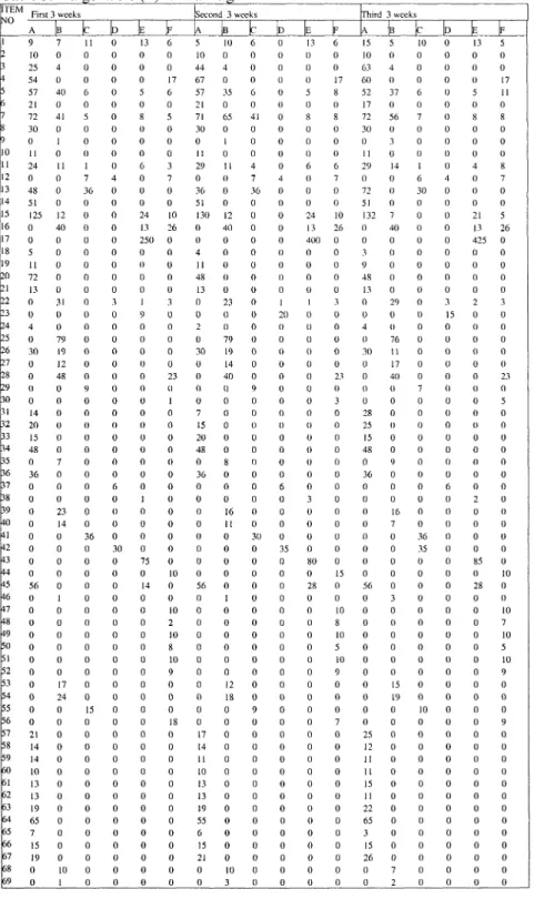
Table 1 shows a list of 69 auto components flovving through a supply chain and forwarded to 6 retail units, denoted as A, B, C, D, E and F down stream, över a 3-week period. The number ordered by each retail unit and the pack sizes are evident

for each component. For instance, 9A means that the retail unit has ordered 9

components of the type shown. As elucidated, there are cases where a retail unit may have ordered the same components (with the same or different quantity) more than önce during the period under consideration, viz 3-week in this case, we add ali the orders as a total.

The quantities were ordered by using a MRP/ERP based system (Ziarati and Khataee, April 1994) as well as a number of empirical equations (rules of thumb). The MRP/ERP system applied did not base its preditions on the past trends. The complexity of the Tables (ie. number of components involved, existing pack sizes, variation in demands by retail units, variation in time of orders and Economic Order Quantities (EOQs), ete, did not allovv for a systematic evaluation of material and information flows through the supply chain. The information used by manufacturers in this case to interact vvith central and regional distribution centres, and the information used betvveen the distribution units and retailers, were not unified and/or integrated through a single database. The knowledge obtained vvas not based on a meaningful learning mechanism of past dealings and activities.

3. TheSolution

The intention here is not to compete with MRP/ERP systems currently used by commercial and industrial organisations. These systems have proven extremely useful (Ziarati, May 1994) in that, pay-off due to their introduetion unlike other high-tech systems viz., CAD, CAM, robotics, ete, has been substantial. As reported in [6] the high pay-offs vvere due to the fact that MRP/ERP systems provide an opportunity for managers to knovv vvhat is going on and hence able to co-ordinate activities vvithin their organisation effectively and efficiently, for instance reduce stoeks.

The intention here is to complement the existing ERP systems. The neural netvvork offers a learning mechanism vvhich could help to predict demand trends more accurately (in terms of material quantities, pack sizes, EOQs, ete.) vvith due consideration for spatial and temporal requirements. There is no reason as to why a neural netvvork ERP should not be a way forvvard in the near future.

An explanation of the neural netvvork approach adopted for this problem is given in the follovving seetion. Immediately after, an explanation is provided as to how data vvas computed and hovv output data vvas obtained.

4. Genetic Cellular Neural Networks

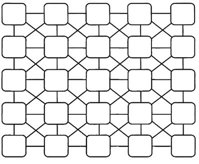
Cellular Neural Netvvorks (CNN) vvere introduced by Chua and Yang (1988). A general CNN neighbourhood structure is sfıovvn in Figüre 1. The CNN structure is vvell suited for the computation of tabulated data (Figures 1&2). The CNN

(4)

normalised differential state-equation can be described by matrix-convolution

operators as:

vvhere U, X, Y are input, state and output of an M x N matrix, while I is an offset

vector. The model used for the input-output relationship is given in Figüre 3. The

feedback and feed-forward connections are represented by matrix A and B.

The relationship betvveen the state and output is non-linear as defined by the

Equation below:

Y„ =o.5|x,.+ı|-|x, -il]*

J ı v I I v M (i)

The characteristics of a CNN celi are governed by piece-vvise variation as elucidated

in Figüre 4. The variation of the CNN output is governed by Equation 1. Therefore,

iteration is stopped only when the derivative of the state variable (dX/dt) becomes

zero, leading to an output value given by:

Y°° = Y.

lJ lJ

(3)

For the CNN to be stable, Aand B should be symmetrical and the centre element of

A must be > 1 for a 3 x 3 matrix. Figüre 5 elucidates the propagation principle of a

two-dimensional CNN.

4.1 Genetic Algorithm

GCNN is a CNN incorporating a Genetic Algorithm (GA). GA is a learning

algorithm vvhich abides by rules of the genetic science. The algorithm has been

successfully applied in a number of cases such as image processing, geophysics, ete.

(Ucan, 2001; Davies, 1991). it uses a binary coding system to search for optimum

values of A, B and I.

The process of natural seleetion causes ehromosomes (in this case, a given set of A,

B and I matrix elements) to be continually reproduced and optimised. in addition to

reproduetion, mutations may cause the off-springs to be different from those of their

biological parents, and erossing över processes create different ehromosomes in

off-springs by changing some parts of the parents' ehromosomes. Like nature, genetic

algorithm solves the problem of finding good ehromosomes by a random

manipulation of the ehromosomes.

The underlying principles of GA were first published by Holland (1962). The

mathematical framevvork was developed in the 1960s and was presented in his

pioneering book (1975). in optimisation applications, they have been used in many

diverse fields such as, funetion optimisation, image processing, travelling sales

person problem, system identification and control and so forth. in machine learning,

GA has been used to learn syntactically simple string IF-THEN rules in an arbitrary

(5)

environment. A high-level description of GA as introduced by Davis in 1991 is

given by [8]. Here, this high level presentation has been used in the prediction of

components requirements in a supply chain as described below:

Stepi: Initialise a population of chromosomes - set a random value to A, B & I.

Step2: Evaluate each chromosome - reproduce viz. assign nevv values to A, B & I.

Step3: Create nevv chromosomes by mating; apply mutation and recombination as

the parent chromosomes mate - optimise values of A, B & I.

Step4: Delete members of the population to make room for nevv ones - destroy

intermediate values.

Step5: Evaluate the nevv chromosomes and insert them into the population

-update the optimised values.

Step6: If dX/dt = 0, then stop and return the best values of A, B and I matrix

elements; othervvise, go to Step 3.

Step 1&2 Constructing initial population and extracting the CNN templates

A chromosome is constructed consisting of the first five elements of matrixes A and

B respectively, and value of I making a total of 11 different values (see equations 4

and 9). The other elements in matrixes A and B respectively have the same values

as the corresponding first five (see equation 9). A given element of matrix A, B and

I value is represented by 7 decimal digits (i.e. -1.3125) hence as a 16 bit register

(memory location) is too small to hold this number, 32 bit registers are required. As

the total number of elements for a chromosome i s l i , therefore a chromosome can

be represented by 32x11= 352 bits (see equation 10). At the start the values for A, B

and I are randomly constructed. in each chromosome the first 32 bits represent the

first element (A 1,1), and the second 32 bits of the chromosome represents the

second element (A 1,2) and so on. There are 11 different values in a given

chromosome as elucidated belovv:

**$ ~ LA.l' A,2 ' A,3 ' A , l ' A,2 ' ^1,1' °1,2 ' ^1,3 ' ^2,1» ^2,2 > * J ,^**

Steps 3 - 6 Optimising chromosome

The CNN works vvith the matrixes of A, B, I belonging to the first chromosome.

After, the CNN output appears as stable, a function is used to obtain the target value.

This function is called the Cost Function vvhich enables the target value to be

computed from the output values. This process is repeated for each set of matrixes

belonging to each chromosome in the population. The Cost Function used in this

study is given belovv:

M N

cost(A,B,I) =

J E £ ( R J - T , J

V i-ı H (5)

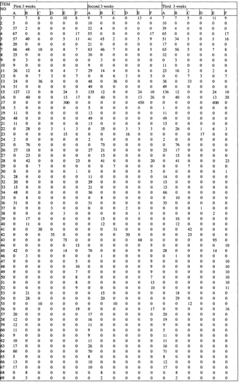
where Pjj and Ty are the elements of Tables 2 and 3 respectively. The elements of

Table 2 give the number of components ordered at any time by a dealer for each

item for the first, second and third "3-week" period. Similarly Table 3 is composed

of the values for the fourth, fifth and sixth "3-vveek" period used as a target matrix

(6)

for training purposes. Having found the Cost Function, the Fitness Function for

each chromosome is determined by the follovving equation:

fitness( A, B, I) =

l + cost(A,B,I)

( 6 )

The eriten on to end iteration is defined as follows:

mincost(A,B,I)<0.01 (7)

where min represents the minimum value of the cost function defined in Equation

(5). If the minimum cost function value (or error) of the chromosome is smaller

than iteration criterion (Equation 7), computation is coneluded and the chromosome

whose fitness value is the maximum in the population is seleeted. The matrixes

which have been extracted from this seleeted chromosome are considered to be the

optimum matrixes.

Creating the next population, the fitness value of the only chromosome is sorted by a

descending order. Ali of the fitness values are normalised in relation to the sum of

the fitness values of the population. A number (R) relating to the normalised values

between 0 and 1 is generated leading to an optimised chromosome.

4.2 Application of GCNN in Demand Predication within a Given Supply Chain

- an Example

This example is based on aetual data obtained in a real supply chain. By using the

data given in Tables 2-5, the following seetions deseribe how the GCNN model

works. First the neural model needs to be trained. The two datasets P and T as

shown in Tables 2 and 3 are used for this purpose. The P dataset consists of the

quantities ordered (69 types of parts) by the six retail units during first 3-week

period. Similarly, T dataset ineludes quantities sold by the six retail units during the

same period. Since the difference between maximum values and the minimum

values of the dataset elements is large (viz., buying and selling some parts in 6s and

7s and some in lOOs), the datasets have been transformed as follovvs:

pı = iog(P + i) n = io

g

(r + i)

( 8 )

The elements of both datasets Pl and Tl are divided by their maximum value. The

same process is applied to the test datasets PP and TT (Table 4 and 5).

in optimisation of A, B and I templates, GA is used. in GA, the chromosomes are

deleted from the population after a given number of iteration (30 in this trials), and

also if their fitness is below a certain threshold set by Equations 5 and 6. This

procedure is known as reproduetion process. Reproduction process does not

generate new chromosomes. it seleets the best chromosomes in the population and

inereases the number of the chromosomes whose fitness values are relatively greater

than the others.

(7)

At the end of the training process and after 143 generation later the following matrixes were found:

-1.3125 -4.1250 -5.1875^ A = \ -6.3750 1.0000 -6.3750 -5.1875 -4.1250 -1.3125 -0.6875 -0.1875 -7.0000" B = \ -6.0625 4.1875 -6.0625 -7.0000 -0.1875 -0.6875 1 = 5.750 (9)

The best chromosome which holds the above values of A, B and I is given by: S=[10000101111001100001000000000011100010001011011110010101011010010 11001100101001001010000000101110110110101101100010101011110110010100 10110110011001000010000010010001100001000011001111110010100011001110 00010100101010000001100101110011010011010110010010000000110101101010 00010110111011000101011101000111101101001111101100011111100101000001 010011000000010] (10) Tables (2-5) are transferred to 2-D image processing form as in Figüre (6-7), where

the values of the dataset elements are shown by varying gray levels in the range of [0,1]. Thus we are able to apply our proposed GCNN approach to the considered supply chain. By using Equations 8-10, we can obtain GCNN output for training and testing as in shovvn in Figures 6 and 7. As a result, we can say that GCNN has promising applications in learning and predicting materıal demand in a supply chain. 5. Conclusions

This paper is an attempt to predict the optimum material and information flow for use by supply chains. A new stochastic algorithm, namely Genetic Cellular Neural Network (GCNN) is proposed. The training procedure is achieved by Genetic Algorithm (GA) which is based on a biological optimisation. Matrixes A and B respectively and the value of I are required for the CNN. Only 11 different matrix element values are necessary; hence computation is based on determining only 11 parameters as against lOOs and sometimes lOOOs parameters needed by other neural network algorisms. Such a limited and small number of parameter requirements make the neural iteration very short compared to other methods.

Application of the existing bitmap and vector graphic techniques (Figures 6 and 7), used in image processing, presented in this paper, should be considered a novel approach in training of the neural netvvorks and their use in predicting material flow in a given supply chain. The bitmap concept has added a third dimension to the tabulated data and the application of vector graphics is expected to enhance the connectivity vvithin the proposed neural network architecture.

(8)

The new approach has promising outcomes in learning and predicting material and also information flow in a supply chain as shown in Figures 6 and 7. it has a potential to become a prediction tool within the existing ERP süite of softvvare or be used for the development of neural ERPs in the near future.

6. References

CHUA, L. O., YANG, L. (1988). "Cellular Neural Networks: Theory", IEEE Trans.

Circuit and Systems, V35, pp.1257-1272.

DAVIS, L., (1991). Handbook of Genetic Algorithms, New York: Van Nostrand Reinhold.

HOLLAND, J.H. (1975). "Outline for a logical theory of adaptive systems: J. Assoc." Computer, v.3, pp.297-314.

. (1975). Adaptation in neural and artificial systems, Ann Arbor, MI: University of the Michigan Press

KOZEK, T., ROSKA, T., CHUA, L.O. (1988). "Genetic Algorithms for CNN template Learning", IEEE Trans. Circuit and Systems, V40, pp.392-402. STOCKTON, D.T., QUINN, L. (1993). "Identifying Economic Order Quantities

Using Genetic Algorithms" International Journal of Operations and Production

Management, v.3, n. 11.

UÇAN, O. et al. (2001). "Separation of Bouguer anomaly map using cellular neural netvvork", Journal of Applied Geophysics 46, pp. 129-142.

WANG, Q. (2000, November), împroving the Cost Model Development Process

Using Neural Networks, Thesis, De Monfort University.

ZIARATI, M., UCAN, O.N. (2001, January). "Optimisation of Economic Order Quantity Using Neural Netvvorks Approach", Dogus University Journal Number, No: 3, pp. 128-140.

ZIARATI, R. (1994, May). "Factories of the Future", Invited paper, EUROTECNET

Conference, Germany

ZIARATI, R., KHATAEE, A. (1994, April). "Integrated Business information System (IBIS) - A Quality Led Approach", Keynote Address. SheMet 94, Belfast University Press, Ulster, UK

LIST OF TABLES:

Table 1. Product descriptions and quantities demanded by the dealers Table 2. Input table (P) for training

Table 3. Output table (T) for training Table 4. Input table (PP) for testing Table 5. Input table (TT) for testing LIST OF FİGURES:

Figüre 1. General CNN neighbourhood structure.

Figüre 2. Representation of neighbourhood relation of CNN. Figüre 3. CNN model input-output relationship.

Figüre 4. Piece-wise linear output characteristics of CNN celi. Figüre 5. CNN propagation effect on 2-D images.

Figüre 6.GCNN Application for training (a) 2-D image form of Table 1 (b) 2-D image form of Table2 (c) GCNN output

Figüre 7.GCNN Application for testing (a) 2-D image form of Table 3(b) 2-D image form of Table 4 (c) GCNN output

(9)

TABLES:

IT EM | S e r v i c e Kit | W i p e r B l a d e B r a k e P a d - F r o n t S e t Oıl Fılter C a n n i s t e r W / S c r e e n W İ p e r B l a d e C a m P l a t e U y d r a u l B r a k e Fluid P A D S e r v i c e Kit | D r ı v e Belt S e r v i c e Kit X J 8 S e r v i c e Kit 3 2 0 0 0 km H S M O Fluid 5 0 0 M L İ F l a n g e L o c k i n g N u t On P l u g I g n i t i o n C O I I.Jracket B u m p e r B l a d e N u m b e r Plate F i x i n g s U n d e r t r a y A s s y W ı s h b o n e B u s h H e x a g o n H e a d Screvv l i u l b H I S 5 W S e r v i c e Kit 1600 km A n t i - R a i d S P A n t i Roll B a r B u s h T H R E A D E D I N S E R T l ' u s h - i n F a s t e n e r ]' C L I P R o k u t R i v e t P o p R i v e t Vee M o u n t i n g C y l i n d e r H e a t Bolt Ziw B a y o n e t L o n g Life | S t u d - E x h a u s t M i f o l d S p a r k P l u g S e r v i c e Kit Brake C l e a n e r S e r v i c e Kit S e r v i c e Kit Fir T r e e l l i p N u t Setscrevv L o c k i n g Bolt Screvv R i v e t J o i n t M a n i f o l d B o l t ( C y l i n d e r B o l t ) S e r v i c e Kit X J 8 A l i e n m e n t G r o m m e t L o c k i n g N u t P l u g - M e t a l S e a l 25 mm 30 mm 40 mm S e a l i n g P l u g Blind R i v e t F e s t o o n B u l b Sw 21/5W B a y o n e t L o n g / L O v a l W A S H E R G r o m m e t B a t t e r y - R o m o t e C T L D a m p e r B u s h B r a k e C o o l D u c t A l t e r n a t i v e D r i v e Belt S L P F L X B U S H İ B u s h U p p e r W i b o n e S y u d C A M C O V E R S E A L KİT İW a t e r B y - p a s s H o s e lEarth L e a d | H4 60/55W L o n g Life İ S e r v i c e Kit X J 8 P A C K O T Y 12 25 4 14 5 5 6 6 5 5 5 14 9A 10A 12A 23A 25A 21A 12A 30A İB H A 4B 4F 48A 51A 42A 13E 300E 5A 13A 36A 13A 8B 16D 4A 81B 19B 17B 48B 9C 3F 14A 25A 20A 24A 7B 36A İ D İE 16B 14B 36C 30D 4 0 E 10F 56A İB 10F 10F 10F 10F 10F U F 2F 1 1 A 12B 8E I4A 2C 12C 10F 40B 200E 36A 4B 24A 4B İD 28E O 3B 5A 22A 21A 13B 3 E 3C 30A 8B u 2C 4B 17F 5E 42A 3F 2C 24E 3 D A 2B 22A 5F 9B 3B 2D 36A 5B N 2C 1 1 A 8C 4C 12B İE T 2F 6B 18A 3 E I 2B 6C 8F 3B T 9B 3F I 13E 13A 6F 23B 15A 3F 24C 42A 26F 3F 30A 23F 40E 17B 24B 15C 18F 21A 14A 14A İ0A 13A 13A 19A 65A 7A 15A 19A 10B İB E 2F 22B 4B 2D 6B s 1 2C

(10)

(11)

(12)

Table 3. Target table (T) for training

İTEİV pjo 1 2 3 4 5 6 7 8 9 10 11 12 13 14 15 16 17 18 19 20 21 22 23 24 25 26 27 28 29 30 31 32

ta

B4 35 B6 B7 B8 B9 ko 41 42 4 3 44 r5 M r ks W9

r°

r1 5 2 r3 r4 r5 r6 r r8 P9 m r r2

p

r4 6 5 6 6 r 1)8 |69 First 3 vveeks _A 9 10 25 54 57 21 72 30 0 11 24 0 48 51 125 0 0 5 11 72 13 0 0 4 0 30 0 0 0 0 14 20 15 48 0 36 0 0 0 0 0 0 0 0 56 0 0 0 0 0 0 0 0 0 0 0 21 14 14 10 13 13 19 65 7 15 19 0 0 İB 7 0 4 0 40 0 41 0 1 0 11 0 0 0 12 40 0 0 0 0 0 31 0 0 79 19 12 48 0 0 0 0 0 0 7 0 0 0 23 14 0 0 0 0 0 1 0 0 0 0 0 0 17 24 0 0 0 0 0 0 0 0 0 0 0 0 0 10 1

±Z

11 0 0 0 6 0 5 0 0 0 1 7 36 0 0 0 0 0 0 0 0 0 0 0 0 0 0 0 9 0 0 0 0 0 0 0 0 0 0 0 36 0 0 0 0 0 0 0 0 0 0 0 0 0 15 0 0 0 0 0 0 0 0 0 0 0 0 0 0

n

0 0 0 0 0 0 0 0 0 0 0 4 0 0 0 0 0 0 0 0 0 3 0 0 0 0 0 0 0 0 0 0 0 0 0 0 6 0 0 0 0 30 0 0 0 0 0 0 0 0 0 0 0 0 0 0 0 0 0 0 0 0 0 0 0 0 0 0 0

UZ

13 0 0 0 5 0 8 0 0 0 6 0 0 0 24 13 250 0 0 0 0 1 9 0 0 0 0 0 0 0 0 0 0 0 0 0 0 1 0 0 0 0 75 0 14 0 0 0 0 0 0 0 0 0 0 0 0 0 0 0 0 0 0 0 0 0 0 0 0

T~

6 0 0 17 6 0 5 0 0 0 3 7 0 0 10 26 0 0 0 0 0 3 0 0 0 0 0 23 0 1 0 0 0 0 0 0 0 0 0 0 0 0 0 10 0 0 10 2 10 8 10 9 0 0 0 18 0 0 0 0 0 0 0 0 0 0 0 0 0 Second 3 vveeks A 5 10 44 67 57 21 71 30 0 11 29 0 36 51 130 0 0 4 11 48 13 0 0 2 0 30 0 ü 0 0 7 15 20 48 0 36 0 0 0 0 0 0 0 0 56 0 0 0 0 0 0 0 0 0 0 0 17 14 11 10 13 13 19 55 6 15 21 0 _0

I£_

10 0 4 0 35 0 65 0 1 0 11 0 0 0 12 40 0 0 0 0 0 23 0 0 79 19 14 40 0 0 0 0 0 0 8 0 0 0 16 11 0 0 0 0 0 1 0 0 0 0 0 0 12 18 0 0 0 0 0 0 0 0 0 0 0 0 0 10 3

±Z

6 0 0 0 6 0 41 0 0 0 4 7 36 0 0 0 0 0 0 0 0 0 0 0 0 0 0 0 9 0 0 0 0 0 0 0 0 0 0 0 30 0 0 0 0 0 0 0 0 0 0 0 0 0 9 0 0 0 0 0 0 0 0 0 0 0 0 0 0

L¥I

0 0 0 0 0 0 0 0 0 0 0 4 0 0 0 0 0 0 0 0 0 1 20 0 0 0 0 0 0 0 0 0 0 0 0 0 6 0 0 0 0 35 0 0 0 0 0 0 0 0 0 0 0 0 0 0 0 0 0 0 0 0 0 0 0 0 0 0 0

ÜZ

13 0 0 0 5 0 8 0 0 0 6 0 0 0 24 13 400 0 0 0 0 1 0 0 0 0 0 0 0 0 0 0 0 0 0 0 0 3 0 0 0 0 80 0 28 0 0 0 0 0 0 0 0 0 0 0 0 0 0 0 0 0 0 0 0 0 0 0 0

iz

6 0 0 17 8 0 8 0 0 0 6 7 0 0 10 26 0 0 0 0 0 3 0 0 0 0 0 23 0 3 0 0 0 0 0 0 0 0 0 0 0 0 0 15 0 0 10 8 10 5 10 9 0 0 0 7 0 0 0 0 0 0 0 0 0 0 0 0 0 rhird A 15 10 63 60 52 17 72 30 0 11 29 0 72 51 132 0 0 3 9 48 13 0 0 4 0 30 0 0 0 0 28 25 15 48 0 36 0 0 0 0 0 0 0 0 56 0 0 0 0 0 0 0 0 0 0 0 25 12 11 11 15 11 22 65 3 15 26 0 0 3 vveeks JB 5 0 4 0 37 0 56 0 3 0 14 0 0 0 7 40 0 0 0 0 0 29 0 0 76 11 17 40 0 0 0 0 0 0 9 0 0 0 16 7 0 0 0 0 0 3 0 0 0 0 0 0 15 19 0 0 0 0 0 0 0 0 0 0 0 0 0 7 _ 2

IE_

10 0 0 0 6 0 7 0 0 0 1 6 30 0 0 0 0 0 0 0 0 0 0 0 0 0 0 0 7 0 0 0 0 0 0 0 0 0 0 0 36 35 0 0 0 0 0 0 0 0 0 0 0 0 10 0 0 0 0 0 0 0 0 0 0 0 0 0 0

_¥I

0 0 0 0 0 0 0 0 0 0 0 4 0 0 0 0 0 0 0 0 0 3 15 0 0 0 0 0 0 0 0 0 0 0 0 0 6 0 0 0 0 0 0 0 0 0 0 0 0 0 0 0 0 0 0 0 0 0 0 0 0 0 0 0 0 0 0 0 0

uz

₁₃ 0 0 0 5 0 8 0 0 0 4 0 0 0 21 13 425 0 0 0 0 2 0 0 0 0 0 0 0 0 0 0 0 0 0 0 0 2 0 0 0 0 85 0 28 0 0 0 0 0 0 0 0 0 0 0 0 0 0 0 0 0 0 0 0 0 0 0 0

~H

5 0 0 17 11 0 8 0 0 0 8 7 0 0 5 26 0 0 0 0 0 3 0 0 0 0 0 23 0 5 0 0 o 0 o 0 0 0 0 0 0 0 0 10 0 0 10 7 10 5 10 9 0 0 0 9 0 0 0 0 0 0 0 0 0 0 0 0 0

(13)

Table 4. Input table (PP) for testing İTEM NO r r r r

p

r

p

r r 10 11 12 13 14 15 16 17 18 19 po pı G2

P

r4

p

p6

r

b

r9 po bı B2 B3 B4 B5

P

6 r7 B8 B9 ko r1 r2 r3 m V5 m r W8 W9

r°

pı p2 p3 r4 p5 p6 r P8 r m r1 B2 P3 r4 K5 66 r

p

(69 First 3 weeks A 7 5 37 67 57 20 66 25 0 9 26 0 24 51 127 0 0 3 11 48 11 0 0 2 0 27 0 0 0 0 28 20 15 48 0 31 0 0 0 0 0 0 0 0 42 0 0 0 0 0 0 0 0 0 0 0 20 12 12 11 9 10 17 60 5 13 17 0 0

_E_

7 0 2 0 40 0 48 0 3 0 12 0 0 0 12 40 0 0 0 0 0 28 0 0 76 18 23 42 0 0 0 0 0 0 8 0 0 0 17 11 0 0 0 0 0 3 0 0 0 0 0 0 21 28 0 0 0 0 0 0 0 0 0 0 0 0 0 8 3

H

8 0 0 0 6 0 10 0 0 0 4 7 36 0 0 0 0 0 0 0 0 0 0 0 0 0 0 0 7 0 0 0 0 0 0 0 0 0 0 0 30 0 0 0 0 0 0 0 0 0 0 0 0 0 10 0 0 0 0 0 0 0 0 0 0 0 0 0 0

IE:

0 0 0 0 0 0 0 0 0 0 0 3 0 0 0 0 0 0 0 0 0 3 0 0 0 0 0 0 0 0 0 0 0 0 0 0 3 0 0 0 0 35 0 0 0 0 0 0 0 0 0 0 0 0 0 0 0 0 0 0 0 0 0 0 0 0 0 0 0

T ~

10 0 0 0 5 0 8 0 0 0 4 0 0 0 24 13 300 0 0 0 0 1 15 0 0 0 0 0 0 0 0 0 0 0 0 0 0 3 0 0 0 0 75 0 14 0 0 0 0 0 0 0 0 0 0 0 0 0 0 0 0 0 0 0 0 0 0 0 0

X I

8 0 0 17 11 0 7 0 0 0 7 7 0 0 5 17 0 0 0 0 0 3 0 0 0 0 0 23 0 1 0 0 0 0 0 0 0 0 0 0 0 0 0 15 0 0 5 10 7 8 8 9 0 0 0 19 0 0 0 0 0 0 0 0 0 0 0 0 0 Second 3 weeks A 9 10 32 53 41 21 63 30 0 9 29 0 48 49 135 0 0 5 13 49 13 0 0 2 0 27 0 0 0 0 11 29 21 36 0 31 0 0 0 0 0 0 0 0 70 0 0 0 0 0 0 0 0 0 0 0 17 16 11 9 9 11 26 70 8 10 10 0 0

ü

7 0 4 0 45 0 46 0 3 0 14 0 0 0 12 40 0 0 0 0 0 35 0 0 75 21 15 41 0 0 0 0 0 0 8 0 0 0 15 12 0 0 0 0 0 1 0 0 0 0 0 0 15 20 0 0 0 0 0 0 0 0 0 0 0 0 0 8 2

_£_

6 0 0 0 2 0 7 0 0 0 4 6 36 0 0 0 0 0 0 0 0 0 0 0 0 0 0 0 7 0 0 0 0 0 0 0 0 0 0 0 31 0 0 0 0 0 0 0 0 0 0 0 0 0 10 0 0 0 0 0 0 0 0 0 0 0 0 0 0

IE:

0 0 0 0 0 0 0 0 0 0 0 3 0 0 0 0 0 0 0 0 0 3 16 0 0 0 0 0 0 0 0 0 0 0 0 0 2 0 0 0 0 30 0 0 0 0 0 0 0 0 0 0 0 0 0 0 0 0 0 0 0 0 0 0 0 0 0 0 0

İ Ü

13 0 0 0 5 0 8 0 0 0 6 0 0 0 24 13 450 0 0 0 0 3 0 0 0 0 0 0 0 0 0 0 0 0 0 0 0 1 0 0 0 0 68 0 9 0 0 0 0 0 0 0 0 0 0 0 0 0 0 0 0 0 0 0 0 0 0 0 0

!EZ

4 0 0 17 9 0 5 0 0 0 6 5 0 0 10 26 0 0 0 0 0 3 0 0 0 0 0 20 0 5 0 0 0 0 0 0 0 0 0 0 0 0 0 9 0 0 9 9 9 7 15 10 0 0 0 17 0 0 0 0 0 0 0 0 0 0 0 0 0 Third A 7 10 39 65 51 17 65 32 0 11 25 0 36 49 136 0 0 1 11 49 13 0 0 2 0 25 0 0 0 0 14 15 15 66 0 35 0 0 0 0 0 0 0 0 28 0 0 0 0 0 0 0 0 0 0 0 20 19 9 5 11 11 16 71 8 12 17 0 0 3 weeks

n

₇ 0 4 0 34 0 56 0 5 0 16 0 0 0 12 40 0 0 0 0 0 26 0 0 76 17 15 41 0 0 0 0 0 0 10 0 0 0 16 12 0 0 0 0 0 1 0 0 0 0 0 0 18 29 0 0 0 0 0 0 0 0 0 0 0 0 0 8 2

±z

₅ 0 0 0 5 0 5 0 0 0 2 7 33 0 0 0 0 0 0 0 0 0 0 0 0 0 0 0 7 0 0 0 0 0 0 0 0 0 0 0 42 25 0 0 0 0 0 0 0 0 0 0 0 0 12 0 0 0 0 0 0 0 0 0 0 0 0 0 0

IE:

0 0 0 0 0 0 0 0 0 0 0 3 0 0 0 0 0 0 0 0 0 1 17 0 0 0 0 0 0 0 0 0 0 0 0 0 1 0 0 0 0 0 0 0 0 0 0 0 0 0 0 0 0 0 0 0 0 0 0 0 0 0 0 0 0 0 0 0 0

m

11 0 0 0 5 0 7 0 0 0 2 0 0 0 24 13 600 0 0 0 0 6 0 0 0 0 0 0 0 0 0 0 0 0 0 0 0 2 0 0 0 0 95 0 14 0 0 0 0 0 0 0 0 0 0 0 0 0 0 0 0 0 0 0 0 0 0 0 0

T\

9 0 0 17 16 0 8 0 0 0 4 7 0 0 10 20 0 o 0 0 0 3 0 0 0 0 0 23 0 1 0 0 0 0 0 0 0 0 0 0 0 0 0 10 0 0 10 10 10 10 10 11 0 0 0 16 0 0 0 0 0 0 0 0 0 0 0 0 0

Design and development of material and information flow for supply chains using genetic cellular networks