Efficient computation of quadratic-phase integrals
in optics
Haldun M. Ozaktas, Aykut Koç,*and Ilkay Sari†
Department of Electrical Engineering, Bilkent University, TR-06800, Bilkent, Ankara, Turkey M. Alper Kutay
TÜBI˙TAK-Scientific and Technological Research Council of Turkey, TR-06100, Kavaklidere, Ankara, Turkey
Received June 29, 2005; revised manuscript received August 22, 2005; accepted September 12, 2005 We present a fastN log N time algorithm for computing quadratic-phase integrals. This three-parameter class of integrals models propagation in free space in the Fresnel approximation, passage through thin lenses, and propagation in quadratic graded-index media as well as any combination of any number of these and is therefore of importance in optics. By carefully managing the sampling rate, one need not chooseN much larger than the space–bandwidth product of the signals, despite the highly oscillatory integral kernel. The only deviation from exactness arises from the approximation of a continuous Fourier transform with the discrete Fourier transform. Thus the algorithm computes quadratic-phase integrals with a performance similar to that of the fast-Fourier-transform algorithm in computing the Fourier transform, in terms of both speed and accuracy. © 2006 Optical Society of America
OCIS codes: 070.2580, 350.6980, 070.2590.
A quadratic-phase system is a unitary system whose output g共u兲 is related to its input f共u兲 through a quadratic-phase integral:
g共u兲 =
冑
exp共− i/4兲 ⫻冕
−⬁ ⬁
exp关i共␣u2− 2uu
⬘
+␥u⬘
2兲兴f共u⬘
兲du⬘
, 共1兲 where␣,, and␥are real parameters. This relation-ship is also known by other names, including “linear canonical transforms.”1–4This input–output relation can model a broad class of optical systems, including thin lenses, sections of free space in the Fresnel approximation, sections of quadratic graded-index media, and arbitrary concat-enations of any number of these.2,3
Computation of the Fresnel diffraction integral, which is a special case of Eq. (1) with␣==␥, has re-ceived the greatest attention because it describes the propagation of light in free space (see Refs. 5 and 6 and the references therein). As the input–output re-lationship represented by the Fresnel integral is space invariant and takes the form of a convolution, one can compute it by taking the Fourier transform (FT) of the input, multiplying by the transfer func-tion of free space, and inverse transforming, with overall time⬃N log N. Here we present an algorithm with which to compute Eq. (1) in ⬃N log N time, de-spite the fact that the relationship represented by the more general Eq. (1) is not space invariant and is not a convolution. It is important to underline that here N is chosen close to the space–bandwidth product of the set of input signals, which is usually the smallest possible value of N that can be chosen in terms of information-theoretic considerations. Therefore the algorithm is highly efficient and, although we do not present a formal proof of this, is quite possibly nearly
the most efficient that is possible. Indeed, the distin-guishing feature of the present approach is the care with which sampling and space–bandwidth product issues are handled. Straightforward use of conven-tional numerical methods can result in inefficiencies either because their complexity is larger than ⬃N log N or because the highly oscillatory quadratic-phase kernel in Eq. (1) forces N to be chosen much larger than the space–bandwidth product of the sig-nals.
In the method presented here, the samples of the output are computed in terms of the samples of the input, in the same sense that the fast-Fourier-transform (FFT) implementation of the discrete Fou-rier transform (DFT) computes the samples of the continuous FT of a function. Special care is taken to ensure that the output samples represent the con-tinuous transform in the Nyquist–Shannon sense, so the continuous transform can be fully recovered from the samples. The only source of deviation from exact-ness arises from the fundamental fact that a signal and its transform cannot both be of finite extent. This is the same source of deviation encountered when the DFT–FFT is used to compute the continuous FT. In-deed, this deviation enters the present algorithm only in the step involving a DFT; all the other steps are fully exact. Therefore the algorithm provides a degree of approximation similar to that of the DFT– FFT and is, in all aspects, to quadratic-phase trans-forms what the DFT–FFT is to the ordinary FT.
Before presenting the algorithm we discuss the Wigner distribution (WD) and the fractional Fourier transform (FRT). The WD, Wf共u,兲, is a phase-space distribution that gives the distribution of signal en-ergy as a function of space and frequency; its defini-tion in terms of f共u兲 may be found elsewhere.2,7The WD of g共u兲 can be simply related to the WD of f共u兲 by a geometrical transformation: Wg共u,兲=Wf共Du−B,
−Cu + A兲, where A=␥/, B = 1 /, C = −+␣␥/, and
January 1, 2006 / Vol. 31, No. 1 / OPTICS LETTERS 35
D =␣/. The FRT Faf共u兲=fa共u兲 is a special case of
quadratic-phase transforms2with ␣=␥= cot共a/ 2兲,  = csc共a/ 2兲, and an additional factor exp共ia/ 4兲 in front of the integral in Eq. (1), for −2艋a艋2. F1is the ordinary Fourier operator and F0 is the identity op-erator. The FRT operator is additive in index: Fa1Fa2=Fa1+a2. We obtain W
fa共u,兲 by rotating Wf共u,兲 by a/ 2.
A function and its FT cannot both be of finite ex-tent. In practice, however, we always work with finite spatial and frequency intervals. We assume that a large percentage of the signal energy, as represented by the WD, is confined to an ellipse with diameters ⌬S (in meters) in the space dimension and ⌬B (in in-verse meters) in the frequency dimension. For a given set of functions we can ensure that this is so by choosing ⌬S and ⌬B sufficiently large. This implies that the space-domain representation of our signal is approximately confined to the interval 关−⌬S/2,⌬S/2兴 and that its frequency-domain repre-sentation is confined to 关−⌬B/2,⌬B/2兴. We then de-fine the space–bandwidth product⌬S⌬B, which is al-ways艌1, because of the uncertainty relation. Let us now introduce scaling parameter s (in meters) and scaled coordinates, such that the space- and frequency-domain representations are confined to in-tervals of length ⌬S/s and ⌬Bs. Let s=
冑
⌬S/⌬B so the lengths of both intervals are equal to the dimen-sionless quantity冑
⌬B⌬S, which we denote by ⌬u, and the ellipse becomes a circle with diameter⌬u. In the new coordinates, our signal can be represented in both domains with ⌬u2 samples spaced ⌬u−1 apart. We assume that this dimensional normalization has been performed and that the coordinates are dimen-sionless.Our method is based on the decomposition of Eq. (1) into elementary operations. Numerous such de-compositions are possible,2 but they are not equally suited for numerical purposes. For instance, the di-rect application of the naïve decomposition of chirp multiplication, Fourier transformation, scaling (mag-nification), and again chirp multiplication that sug-gests itself on inspection of Eq. (1) will in general
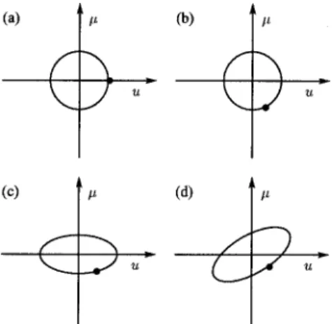
lead to high sampling rates. Our method relies on de-composition into a FRT, magnification, and chirp multiplication. These operations geometrically corre-spond to rotation, scaling, and shearing in the space-frequency plane (Fig. 1). This decomposition was in-spired by the optical interpretation in Ref. 8 and is also a special case of the Iwasawa decomposition. Mathematically,
g共u兲 = exp共− ia/4兲exp共− iqu2兲f
sc共u兲, 共2兲 fsc共u兲 =
冑
1/Mfa共u/M兲, 共3兲 where fa共u兲 is the FRT of f共u兲 anda =共2/兲arccot␥, 共4兲
M =
再
冑
1 +␥2/ ␥艌 0
−
冑
1 +␥2/ ␥⬍ 0冎
, 共5兲 q =␥2/共1 +␥2兲 −␣. 共6兲 The ranges of the square root and the arccotangent both lie in共−/ 2 ,/ 2兴. The first operation in this de-composition is the FRT, whose fast computation in ⬃N log N time is presented in Ref. 9. In the research reported in Ref. 9, the FRT was efficiently computed by being decomposed into a chirp multiplication fol-lowed by a chirp convolution folfol-lowed by a final chirp multiplication. The algorithm computed the samples of the continuous FRT in terms of the samples of the original signal. Just as in the present research, care was taken to ensure that the output samples repre-sented the continuous FRT in the Nyquist–Shannon sense. Our algorithm calls the algorithm in Ref. 9 as a subroutine. The only approximation in this subrou-tine comes from the step involving chirp convolution in which a DFT–FFT is used to approximate the samples of the continuous FT. No other approxima-tion is made, either in this subroutine or in any of the other operations that we employ in our method. Thus the only source of approximation can be traced to the evaluation of a continuous FT by use of a DFT (imple-mented with a FFT), which is a consequence of the fundamental fact that the signal energy cannot be confined to finite intervals in both domains. Thesec-Fig. 1. Decomposition of an arbitrary quadratic-phase sys-tem: (a) region to which the signal energy is initially con-fined, (b) energy distribution after rotation, (c) after scal-ing, (d) final distribution of signal energy after shearing.
Fig. 2. rms errors versus N. Inset, rms error percentages.
ond operation in our decomposition is scaling, which is actually not a real operation but involves only a re-interpretation of the same samples with a scaled sampling interval. The final operation is chirp multi-plication, which takes⬃N time, leading to an overall complexity of ⬃N log N. However, there is one final subtlety that must be taken into consideration. Be-cause quadratic-phase systems distort the original region, as shown in Fig. 1, both the space and the fre-quency extent of the signal as well as its space– bandwidth product may increase, despite the fact that the area of the region remains the same. There-fore, unless some sophisticated basis is used, a greater number of samples than⌬u2may be needed to represent g共u兲.
Delaying confrontation of the necessity to deal with this greater number of samples until the very last step is another advantage of our method. Because the FRT corresponds to rotation and scaling only to rein-terpretation of the samples, these steps do not re-quire us to increase the number of samples. At the last chirp multiplication step, if we multiply the samples of the intermediate result by the samples of the chirp, the samples obtained will be good approxi-mations of the true samples of g共u兲 at that sampling interval. If these samples are sufficient for our pur-poses, nothing further need be done. However, in gen-eral these samples will be below the Nyquist rate for g共u兲 and will not be sufficient for full recovery of the continuous function. To obtain a sufficient number of samples that will permit full recovery, we must inter-polate the intermediate result by at least a factor of k, corresponding to the increase in space–bandwidth product:
k = 1 +兩␥−␣共1 +␥2兲/2兩. 共7兲 Although this formula is sufficient for the approach here, where by careful design the necessity for in-creasing the number of samples has been postponed to the final step, we note that a systematic approach to determining the increase in the number of samples for arbitrary operations has been presented in Ref. 10, which also brings a number of different perspec-tives to the same problem.
Consider the chirped pulse function (F1) (Fig. 2) exp共−u2− iu2兲 and the trapezoidal function (F2) 1.5 tri共u/3兲−0.5 tri共u兲, whose transforms have been computed both by the fast method presented here and by a highly inefficient brute-force numerical ap-proach that is taken here as a reference 关tri共u兲 = rect共u兲*rect共u兲兴. Because these functions are well confined to a circle with diameter ⌬u=8 we take N = 82. We also consider the binary sequence (F3) 01101010 occupying 关−8,8兴, with each bit two units in length, such that N = 162. Also consider two trans-forms, the first (T1) with parameters 共␣,,␥兲=共−3, −2 , −1兲 (leading to k=1.5) and the second (T2) with parameters共−4/5,1,2兲 (leading to k=7). The results
are tabulated in the inset of Fig. 2. We note that the errors are in line with the errors in approximating the FT with the DFT. Figure 2 shows the error versus the number of sample points; the error decreases to-ward the space–bandwidth product but saturates af-terward, demonstrating that we can choose the num-ber of points to be comparable to the space– bandwidth product.
In conclusion, we have presented a fast, ⬃N log N algorithm for computing any quadratic-phase inte-gral. Our approach is based on concepts from signal analysis and processing rather than on conventional numerical analysis. With careful consideration of sampling issues, N can be chosen close to the space– bandwidth product of the signals. The only source of error is that which arises from the approximation of a FT with the DFT. Thus the algorithm can compute quadratic-phase integrals with a performance similar to that of the FFT algorithm in computing the FT, in terms of both speed and accuracy. This approach not only handles a much more general family of integrals but also effectively addresses certain difficulties, limitations, or trade-offs that arise in other ap-proaches to computing the Fresnel integral (see Ref. 10 for a systematic comparison of several ap-proaches). The presented algorithm can also be used for efficient realization of filtering in linear canonical transform domains.11
We thank one of the anonymous reviewers for bringing the recent Ref. 10 to our attention. H. M. Ozaktas ([email protected]) acknowledges partial support of the Turkish Academy of Sciences.
*A. Koc is currently with the Department of Elec-trical Engineering, Stanford University, Stanford, California 94305.
†
I. Sari is currently with the Department of Elec-trical Engineering, Texas A&M University, College Station, Texas 77843.
References
1. K. B. Wolf, Integral Transforms in Science and
Engineering (Plenum, 1979).
2. H. M. Ozaktas, Z. Zalevsky, and M. A. Kutay, The
Fractional Fourier Transform with Applications in Optics and Signal Processing (Wiley, 2001).
3. M. J. Bastiaans, J. Opt. Soc. Am. 69, 1710 (1979). 4. S. Abe and J. T. Sheridan, Opt. Lett. 19, 1801 (1994). 5. D. Mendlovic, Z. Zalevsky, and N. Konforti, J. Mod.
Opt. 44, 407 (1997).
6. D. Mas, J. Garcia, C. Ferreira, L. M. Bernardo, and F. Marinho, Opt. Commun. 164, 233 (1999).
7. L. Cohen, Time-Frequency Analysis (Prentice-Hall, 1995).
8. H. M. Ozaktas and M. F. Erden, Opt. Commun. 143, 75 (1997).
9. H. M. Ozaktas, O. Arıkan, M. A. Kutay, and G. Bozdag˘ı, IEEE Trans. Signal Process. 42, 2141 (1996). 10. B. M. Hennelly and J. T. Sheridan, J. Opt. Soc. Am. A
22, 917 (2005).
11. B. Barshan, M. A. Kutay, and H. M. Ozaktas, Opt. Commun. 135, 32 (1997).