DETERMINATION OF THE OPTIMAL LOCATION OF A 2-DOF MANIPULATOR FOR MINIMAL ENERGY
CONSUMPTION DURING A PREDEFINED TASK Mehmet Beşir KOPMAZ
Master of Science Thesis
Department of Mechatronics Engineering Asst. Prof. Dr. İsmail BÜTÜN
T.R.
BURSA TECHNICAL UNIVERSITY
GRADUATE SCHOOL OF NATURAL AND APPLIED SCIENCES
DETERMINATION OF THE OPTIMAL LOCATION OF A 2-DOF MANIPULATOR FOR MINIMAL ENERGY CONSUMPTION DURING A
PREDEFINED TASK
A THESIS FOR THE DEGREE OF MASTER OF SCIENCE
Mehmet Beşir KOPMAZ
Department of Mechatronics Engineering
Bursa March 2016
MASTER THESIS EXAMINATION RESULT FORM
The thesis entitled “Determination of the Optimal Location of a 2-DoF Manipulator for Minimal Energy Consumption During a Predefined Task” completed by Mehmet Beşir KOPMAZ under supervision of Asst. Prof. İsmail BÜTÜN has been reviewed in terms of scope and quality and approved as a thesis for the degree of Master of Science.
Jury Members
Asst. Prof. İsmail BÜTÜN (Bursa Technical University,
Department of Mechatronics Engineering) ………
Assoc. Prof. Hakan GÖKDAĞ (Bursa Technical University,
Department of Mechanical Engineering) ………
Asst. Prof. Gürsel ŞEFKAT (Uludağ University,
Department of Mechanical Engineering) ………
Date of Examination: 15/03/2016
Director of Graduate School of Natural and Applied Sciences
DECLARATION ON PLAGIARISM
I hereby declare that this piece of written work is the result of my own independent scholarly work, and that in all cases material from the work of others is acknowledged, and quotations and paraphrases are clearly indicated. No material other than listed has been used. I am aware of what constitutes an act of plagiarism and understand that my thesis will be rejected if found to contain any instance of plagiarism.
Student Name and Surname: Mehmet Beşir KOPMAZ Signature:
ACKNOWLEDGEMENTS
I would like to express my deepest gratitude to my advisor, Assistant Professor İsmail BÜTÜN. I have been amazingly fortunate to have an advisor who gave me the freedom to explore on my own, and at the same time the guidance to recover when my steps faltered. His patience and support helped me overcome many crisis situations and finish this thesis. I hope that one day I would become as good an advisor to my students as he has been to me.
My sincere gratitude is also to Professor Osman Kopmaz who has been always there to listen and give advice, encouraging me throughout this endeavor. I am deeply grateful to him for the long discussions that helped me sort out the technical details of my work. I am also thankful to him for encouraging the use of correct grammar and consistent notation in my writings and for carefully reading and commenting on countless revisions of this manuscript.
Most importantly, none of this would have been possible without the love and patience of my family, to whom this thesis is dedicated to. They have been a shelter for me in the confinement of humanity in this corner of the cosmos with their love, concern, support and optimism all these years; a chance to feel special, rather than to be crushed by the weight and beauty of our own loneliness.
v TABLE OF CONTENTS
Page No. Outer Cover
Inner Cover
Master Thesis Examination Result Form Declaration on Plagiarism
Acknowledgements
Table of Contents v
List of Figures vi
List of Symbols viii
Özet xi Abstract xii 1.INTRODUCTION 1 2.LITERATURE SEARCH 2 3.INVERSE ANALYSIS 5 3.1.Position Analysis 6 3.2.Velocity Analysis 7 3.3.Acceleration Analysis 8
4.DEFINITION OF TASK AND SEARCHING OPTIMAL TRAJECTORY 9 5.KINEMATIC CONSTRAINTS, VELOCITY AND ACCELERATION
FUNCTIONS 15
6.EQUATIONS OF MOTION 16
7.SOLVING EQUATION OF MOTION FOR ACTUATOR TORQUES 21
8.CALCULATION OF ENERGY CONSUMPTION 22
9.NUMERICAL EXAMPLES 23
10.CONCLUSION 45
REFERENCES 46
vi LIST OF FIGURES
Figure 3.1 Manipulator of interest 5
Figure 4.1 Geometric definition of trajectory 10
Figure 4.2 The longest possible trajectory 11
Figure 4.3 New coordinate system with respect to minimal energy trajectory 14 Figure 9.1 Position angles of links in Example 1 25 Figure 9.2 Angular velocities of links in Example 1 25 Figure 9.3 Angular accelerations of links in Example 1 26 Figure 9.4 Actuator torques of links in Example 1 26 Figure 9.5 Actuator powers of links in Example 1 27 Figure 9.6 Position angles of links in Example 2 28 Figure 9.7 Angular velocities of links in Example 2 29 Figure 9.8 Angular accelerations of links in Example 2 29 Figure 9.9 Actuator torques of links in Example 2 30 Figure 9.10 Actuator powers of links in Example 2 30 Figure 9.11 Energy consumptions for both configurations in Example 2 31 Figure 9.12 Position angles of links in Example 3 32 Figure 9.13 Angular velocities of links in Example 3 33 Figure 9.14 Angular accelerations of links in Example 3 33 Figure 9.15 Actuator torques of links in Example 3 34 Figure 9.16 Actuator powers of links in Example 3 34 Figure 9.17 Energy consumptions for both configurations in Example 3 35 Figure 9.18 Position angles of links in Example 4 36 Figure 9.19 Angular velocities of links in Example 4 37 Figure 9.20 Angular accelerations of links in Example 4 37 Figure 9.21 Actuator torques of links in Example 4 38 Figure 9.22 Actuator powers of links in Example 4 38 Figure 9.23 Energy consumptions for both configurations in Example 4 39 Figure 9.24 Position angles of links in Example 5 40 Figure 9.25 Angular velocities of links in Example 5 41 Figure 9.26 Angular accelerations of links in Example 5 41 Figure 9.27 Actuator torques of links in Example 5 42 Figure 9.28 Actuator powers of links in Example 5 42
vii
Figure 9.29 Energy consumptions for both configurations in Example 5 43 Figure 9.30 The optimal loci of the root of manipulator in the XY coordinate system 44
viii LIST OF SYMBOLS AND ACRONYMS
Symbol Definition
𝐼1,𝑂 Mass moment of inertia of link 1 with respect to point 𝑂 𝐼2,𝐴 Mass moment of inertia of link 2 with respect to point 𝐴 𝐼𝐺1 Mass moment of inertia of link 1 with respect to point 𝐺1 𝐼𝐺2 Mass moment of inertia of link 2 with respect to point 𝐺2
𝐿 Length of trajectory
𝐿𝑚𝑎𝑥 Maximum possible length of trajectory
𝐿1 Length of link 1
𝐿2 Length of link 2
𝐌𝟏 Torque vector of actuator 1 𝑀1 Torque of actuator 1
𝑀11 Torque of actuator 1 for configuration 1 𝑀12 Torque of actuator 1 for configuration 2 𝐌𝟐 Torque vector of actuator 2
𝑀2 Torque of actuator 2
𝑀21 Torque of actuator 2 for configuration 1 𝑀22 Torque of actuator 2 for configuration 2
𝑃1 Power of actuator 1
𝑃11 Power of actuator 1 for configuration 1 𝑃12 Power of actuator 1 for configuration 2
𝑃2 Power of actuator 2
𝑃21 Power of actuator 2 for configuration 1 𝑃22 Power of actuator 2 for configuration 2 𝑇 Total kinetic energy of manipulator 𝑇1 Kinetic energy of link 1
𝑇2 Kinetic energy of link 2
ix
𝑊 Total virtual work of actuator torques 𝑊1 Virtual work done on link 1
𝑊2 Virtual work done on link 2
𝑟𝐺1 Distance of center of gravity of link 1 from point 𝑂 𝑟𝐺2 Distance of center of gravity of link 2 from point 𝐴
𝑠(𝑡) Motion program
𝑠̇(𝑡) First time derivative of motion program 𝑠̈(𝑡) Second time derivative of motion program 𝐯𝐴 Velocity vector of point 𝐴
𝐯𝐵 Velocity vector of point 𝐵 𝑣𝐵 Linear speed of point 𝐵
𝐯𝐵 𝐴⁄ Velocity vector of point 𝐵 with respect to point 𝐴 𝐯𝐺1 Velocity vector of point 𝐺1
𝑣𝐺1 Linear speed of point 𝐺1 𝐯𝐺2 Velocity vector of point 𝐺2 𝑣𝐺2 Linear speed of point 𝐺2
𝐯𝐺2⁄𝐴 Velocity vector of point 𝐺2 with respect to point 𝐴 𝐮 Trajectory direction unit vector
𝑥 Abscissa of a generic point on the trajectory 𝑥̇ x-component of end point velocity
𝑥̈ x-component of end point acceleration 𝑥𝐹 Abscissa of final point of trajectory 𝑥𝑆 Abscissa of starting point of trajectory 𝑥𝑆𝑖𝑛𝑖𝑡 Initial abscissa of starting point 𝑥𝑆𝑓𝑖𝑛 Final abscissa of starting point
𝑦 Ordinate of a generic point on the trajectory 𝑦̇ y-component of end point velocity
x
𝑦𝐹 Ordinate of final point of trajectory 𝑦𝑆 Ordinate of starting point of trajectory 𝜃1 Position angle of link 1
𝜃11 Position angle of link 1 for configuration 1 𝜃12 Position angle of link 1 for configuration 2 𝜃2 Position angle of link 2
𝜃21 Position angle of link 2 for configuration 1 𝜃22 Position angle of link 2 for configuration 2 𝜃̇1 Angular speed of link 1
𝜃̇11 Angular speed of link 1 for configuration 1 𝜃̇12 Angular speed of link 1 for configuration 2 𝜃̇2 Angular speed of link 2
𝜃̇21 Angular speed of link 2 for configuration 1 𝜃̇22 Angular speed of link 2 for configuration 2 𝜃̈1 Angular acceleration of link 1
𝜃̈11 Angular acceleration of link 1 for configuration 1 𝜃̈12 Angular acceleration of link 1 for configuration 2 𝜃̈2 Angular acceleration of link 2
𝜃̈21 Angular acceleration of link 2 for configuration 1 𝜃̈22 Angular acceleration of link 2 for configuration 2 𝜑 Direction angle of trajectory
𝜑𝑖𝑛𝑖𝑡 Initial direction angle of trajectory 𝜑𝑓𝑖𝑛 Final direction angle of trajectory
Acronym Definiton
xi ÖZET
ÖNGÖRÜLEN BİR GÖREV SIRASINDA EN AZ ENERJİ SARFİYATI İÇİN İKİ SERBESTLİK DERECELİ BİR MANİPÜLATÖRÜN OPTİMUM
KONUMUNUN TAYİNİ Mehmet Beşir KOPMAZ Bursa Teknik Üniversitesi
Fen Bilimleri Enstitüsü Mekatronik Mühendisliği Bölümü
Yüksek Lisans Tezi Yrd. Doç. Dr. İsmail BÜTÜN
Mart 2016, 47 Sayfa
Geçen birkaç on yılda robot manipülatörler verimli, hassas ve hızlı üretime olan devasa katkılarından ötürü seri üretimin vazgeçilemez unsuru haline gelmiştir. Öte yandan, enerjinin verimli kullanımının sınırlı enerji kaynakları ve bunların jeopolitik konumlarından ötürü birinci sanayi devriminden bugüne ana meselelerden biri olduğu iyi bilinen bir gerçektir. Enerjinin en büyük kullanıcılarından birinin imalat sanayi olduğu göz önüne alındığında üretim araçlarının ve bu bağlamda özellikle robotların zaman ve enerji bakımından optimal kullanımının önemi kolayca kavranabilir. Bu sebepten robotbilimde muhtelif kısıtlara maruz yörünge planlama başlığı altında ilgi çekici bir araştırma alanı ortaya çıkmıştır. Bu tez de verilen bir görev ve yörünge için enerji sarfiyatını en aza indirmeyle alakalıdır. Bu araştırma enerji sarfiyatını yeri belirlenmiş bir yörüngeye göre manipülatöre uygun bir yer bularak minimum yapmayı hedeflemesiyle önceki çalışmalardan farklılık arz etmektedir. Bu çalışmada yörüngelerin doğru parçaları şeklinde olduğu kabul edilmiştir. Ayrıca düzgün kinematik karakteristikleri olan sikloidal ve 3-4-5 polinom tipinde iki farklı hareket kanunu kullanılmaktadır. Sayısal sonuçlar manipülatör için enerji sarfiyatını minimum edecek tarzda her halükarda optimal bir konum bulmanın mümkün olduğunu ve 3-4-5 polinom hareket kanununun daha az enerji sarfiyatı sağladığını açıkça göstermektedir. Anahtar Sözcükler: İki uzuvlu düzlemsel manipülatör, minimum enerji sarfiyatı, bir manipülatörün optimal konumu
xii ABSTRACT
DETERMINATION OF THE OPTIMAL LOCATION OF A 2-DOF MANIPULATOR FOR MINIMAL ENERGY CONSUMPTION DURING A
PREDEFINED TASK Mehmet Beşir KOPMAZ Bursa Technical University
Graduate School of Natural and Applied Sciences Department of Mechatronics Engineering
Master of Science Thesis Asst. Prof. Dr. İsmail BÜTÜN
March 2016, 47 Pages
In the past several decades, robot manipulators have been indispensable part of serial production due to their huge contribution to the efficient, accurate and rapid manufacturing. On the other hand, it is a well-known fact that the efficient use of energy has been the main challenge from the first industrial revolution to date due to limited energy resources and their geo-political locations on the world. Considering that one of the largest consumers of energy is manufacturing industry, the importance of time- and energy-optimal usage of production machinery, specifically in this context can be well figured out. For this reason, in the field of robotics, an interesting research area has emerged under the headline of trajectory planning subject to different constraints among which time-optimal, energy-optimal or smooth (jerk- and impact-free) path tracking can be mentioned at first glance. This thesis is concerned with minimizing the energy consumption for a given task and trajectory. The present study differs from the previous work in that energy consumption is minimized by obtaining an appropriate location for the manipulator with respect to the trajectory fixed in the world coordinates. In this work, trajectories are assumed to be straight-lines. Besides, two different motion programs known with their smooth kinematic characteristics are tested, which are the cycloidal and the 3-4-5 polynomial motion programs. Numerical results obviously demonstrate that obtaining an optimal location for the manipulator regarding the use of minimal energy is possible, and the 3-4-5 polynomial motion program provides less energy consumption levels.
xiii
Keywords: 2-DoF planar manipulator, minimum energy consumption, optimal location of a manipulator
1 1. INTRODUCTION
In the past several decades, robots have become indispensable part of production lines due to their huge contribution to the efficient, accurate and rapid manufacturing. As a consequence of this, the trajectory planning subject to different constraints emerged as a new research area. Among them, time-optimal, energy-optimal or jerk-free trajectory planning can be mentioned at first glance. No doubt, energy resources and their efficient use have been the main challenge since the first industry revolution going back to the mid-19th century. Considering that one of large consumers of energy is manufacturing industry, the importance of time- and energy-optimal usage of robots can be well figured out. Although the subject has a long history extending to 1990’s, it is still on the focus of researchers as the extensive literature on the subject indicates. However, to the author’s knowledge, papers on energy-optimal path planning mostly deal with the problems in which starting, final and intermediate points of possible trajectory are given while the robot stands fixed. Some of the relevant papers develop and propose new methods that include almost all the parameters from the physical to control-related ones. These methods usually lead to fairly sophisticated optimization problems.
This thesis is concerned with the energy consumption of a 2-DoF planar manipulator. However, the present study differs from the previous work mainly in its conceptual novel approach. In this work, the position of production line is assumed to be stationary while the location of the manipulator can be changed in such a manner that the energy expenditure is reduced. In some sense, an inverse problem compared to the present literature is posed. Hence, the main purpose of this work is to find the suitable location of the manipulator for a predefined task so that the energy consumption be minimum. To make the proposed novel approach easily understandable, effects such as control parameters, damping, etc. are not considered. The numerical results obtained show that energy-optimal location is feasible for manipulators to be used in fixed production lines. The content of the work is limited with the solution of this problem for a 2-DoF planar manipulator.
2 2. LITERATURE SEARCH
As emphasized in the introduction, minimal energy based trajectory planning continues to be dealt with by researchers. As an indicator of this, here, some mentioning-worth publications from the old to the recent ones will be referred to. In [1], Kopmaz et al. investigated the problem of finding an energy-optimal parabolic trajectory for a certain task which has some kinematic constraints in the start and end point of the trajectory. They used a finite number of trajectories which are defined with a parabolic equation on a pre-determined plane within the work space of a 6-DoF revolute manipulator, and showed that it is possible to find such a trajectory. Diken studied a similar problem in [2] using a sinusoidal path. Alshahrani et al. treated the problem of finding optimal trajectory function for minimum energy requirements of spherical robot, [3]. They assumed that the object to be manipulated follows a straight line in the work space. They choose three different displacement functions: simple harmonic, cycloidal and 3-4-5 polynomial. Compared to the energy consumption for bang-bang parabolic blend type displacement and cubic segment functions, the authors find out that cycloidal and 3-4-5 polynomial functions are tracked with more energy consumption while they provide a smooth running for the robot. If the energy consumption is the prime concern and the travel time is short, cubic segment trajectory is the best choice. Saramago et al. dealt with obtaining a trajectory subject to additional constraints for a PUMA-like robot such that a hybrid objective function consisting of weighted actuator powers and end effector grasping energy takes a minimum value, [4]. In [5], Verscheure et al. handled the problem of time-energy optimal path tracking. An objective function in which time does not appear explicitly is used. Through a nonlinear change of variables, the problem is transformed into a convex optimal control problem. De Santos et al. studied the energy required for six-legged robots which use alternating tripod gaits, and present a method aiming at reducing this energy need, [6]. Chen and Liao developed a hybrid strategy for the time- and energy-efficient trajectory planning for a 6-6 parallel platform, [7]. To this end, they proposed a cost function which consists of weighted functions of the consumed energy and time. In order to ensure the practical feasibility of the planned optimal trajectory, they took the physical constraints imposed by the parallel platform and actuator mechanism on the motion of the platform. The authors used the particle swarm optimization algorithm to obtain a crude estimate of the global optimal trajectory which is then supplied to the
3
conjugate gradient optimization method. They showed that this hybrid strategy outperforms the standalone particle swarm technique. In [8], Gasparetto et al. addressed the general problem of trajectory planning in Robotics. They give an overview of the most important methods proposed in the relevant literature especially to generate collision-free paths. In this work, it is expressed that the minimum time trajectory planning is very significant but this criterion certainly does not exhaust the possible applications or respond to all needs. In this context, the trajectory planning based on energy criteria has many interesting aspects. Such a planning produces smooth trajectories being easier to track and reduce the stresses to the actuators and the manipulator structure. In addition to that this approach allows energy saving which is very important for the cases in which energy source is limited like robotic applications for underwater exploration in military tasks. Gregory et al., [9], investigated the issue of energy-optimal trajectory planning for robot manipulators with holonomic constraints. The authors employ a methodology to transform a variational problem with constraints to the one with no constraints. Hence, the problem take the form of an optimal control problem. They solved the problem on a simple SCARA robot which is a 2-DoF planar manipulator. They found solutions for different constraint types. In [10], Pellicciari et al. proposed a novel method implementable on both serial and parallel robots to minimize energy consumption which works in pick-and-place mode, and the trajectories of which are given by their starting, final and intermediate points. Mohammed et al. developed a different approach to minimize energy consumption. They carried out three scenarios with and without payload, and compared the results with those of commercial simulation software of the robot of interest. They developed a model searching the location of the energy-optimal path, [11]. Fung and Cheng dealt with a trajectory planning problem. They used the basic criterion of minimum absolute input energy (MAIE) to find the sought trajectory. The motion programs they used are parabolic blends, cycloidal, zero-jerk and polynomial ones. The polynomial was chosen of 12nd degree. The coefficients of this polynomial are obtained such that all the boundary conditions for the remaining three different trajectory profiles are satisfied. Then, energy consumptions for each profile are compared with each other. The authors use the real-coded genetic algorithm to find the energy optimal-polynomial for each case, [12]. Paes et al. determined the system parameters of an industrial ABB robot experimentally to find its energy efficient trajectories for a certain task. As a small case study, a typical pick-and-place maneuver
4
is both time- and energy-optimized. The authors subsequently compared these optimal trajectories to several straight-forward trajectories that are indicative for rotor operations in industry. To this end, they used the ACADO toolkit, an algorithm collection for automatic control and dynamic optimization. They proposed a non-invasive identification strategy for industrial robots, [13].
All the works mentioned above demonstrate that the energy consumption of robot manipulators will be a crucial topic in production activities when the issue of energy saving is considered to be of increasing significance. For this reason, in this thesis, energy optimization in manipulators are handled in a different way. For the case to be studied here, the trajectory is assumed to be a straight-line. However, for speed profile, two different functions are employed provided that they have same kinematic constraints. In contrast with the previous work, the energy-optimal location of the manipulator is sought under the assumption that the manipulation path is fixed in the world coordinates. Simulations and computational results show that there exist such optimal locations. For this purposes, a 2-DoF planar manipulator is considered. The choice of such a manipulator is only for simplicity because the first aim is to show how to work the methodology presented here. Firstly, an inverse kinematic analysis will be done. Meanwhile, the trial trajectories will be defined with its all kinematic parameters in such a manner that they are within the work space of the manipulator. Subsequently, for possible configurations of the robot, the energy consumption will be computed for different speed and acceleration profiles and constraints. Finally, the numerical results will be presented in graphics and commented.
5 3. INVERSE ANALYSIS
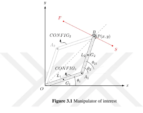
We consider the manipulator shown in Figure 3.1.
Figure 3.1 Manipulator of interest
For a generic point 𝑃(𝑥, 𝑦) in the xy-plane, there exist two different configurations of the manipulator, which are indicated with the abbreviations 𝐶𝑂𝑁𝐹𝐼𝐺1 and 𝐶𝑂𝑁𝐹𝐼𝐺2 in Figure 3.1 respectively. Furthermore, the straight-line SF is the trajectory to be followed by the end effector of the robot. Points S and F are the start and end points of the trajectory. 𝐿1 and 𝐿2 are the length of manipulator links. It is obvious that the work space is an annular region which is bounded by an outer circle with radius of 𝐿1 + 𝐿2 and an inner circle with radius of |𝐿1− 𝐿2|. In practice, this region may be slightly different from the theoretical one due to physical constraints. In Figure 3.1, 𝜃1 and 𝜃2 are absolute rotation angles of two links in the world coordinates. However, the control angle of the second link is 𝜃21 in practical applications.
6 3.1. Position Analysis
From Figure 3.1, the following equations are easily written:
𝐿1cos 𝜃1 + 𝐿2cos 𝜃2 = 𝑥 (3.1a) 𝐿1sin 𝜃1+ 𝐿2sin 𝜃2 = 𝑦 (3.1b) First, angle 𝜃1 is to be formulated. Therefore, the terms including 𝜃2 are left alone on the right side of the equations.
𝐿2cos 𝜃2 = 𝑥 − 𝐿1cos 𝜃1 (3.2a) 𝐿2sin 𝜃2 = 𝑦 − 𝐿1sin 𝜃1 (3.2b) Taking square of both sides and adding side by side, the equation below is obtained:
𝐿22 = 𝑥2 + 𝑦2+ 𝐿21− 2𝑥𝐿1cos 𝜃1− 2𝑦𝐿1sin 𝜃1 (3.3a) Rearranging 3.3a it we obtain:
−2𝑥𝐿1cos 𝜃1 − 2𝑦𝐿1sin 𝜃1+ 𝑥2+ 𝑦2+ 𝐿21− 𝐿22 = 0 (3.3b) Let us define: 𝑎 ≔ −2𝑥𝐿1 𝑏 ≔ −2𝑦𝐿1 𝑐 ≔ 𝑥2+ 𝑦2+ 𝐿21− 𝐿22 𝜆 ≔ tan𝜃1 2 (3.4a) (3.4b) (3.4c) (3.4d) As is well-known from trigonometry, the following relationships exist:
cos 𝜃1 = 1 − 𝜆 2
1 + 𝜆2 (3.5a)
sin 𝜃1 = 2𝜆
1 + 𝜆2 (3.5b)
Using (3.4) and (3.5) in (3.3b) one finds:
(1 − 𝜆2)𝛼 + 2𝑏𝜆 + (1 + 𝜆2)𝑐 = 0 (3.6a) or
7 Now, similar to the first three of (3.4), we define
𝐴 ≔ 𝑐 − 𝑎 𝐵 ≔ 𝑏 𝐶 ≔ 𝑐 + 𝑎 (3.7a) (3.7b) (3.7c) Substituting (3.7) in (3.6) gives the equation
𝐴𝜆2+ 2𝐵𝜆 + 𝐶 = 0 (3.8)
the roots of which are
𝜆1 = −𝐵 − √𝐵2− 𝐴𝐶 𝐴 (3.9a) 𝜆2 =−𝐵 + √𝐵 2− 𝐴𝐶 𝐴 (3.9b)
respectively. Hence we have two distinct values for 𝜃1:
𝜃1,1 = 2 tan−1𝜆1 (3.10a)
𝜃1,2= 2 tan−1𝜆2 (3.10b)
where the second subscript refers to these distinct values of 𝜃1, which implies that these exist two possible configurations of the robot to reach point 𝑃. From equation (3.2), the variants of 𝜃2 can be found as follows:
sin 𝜃2,𝑖 =𝑦 − 𝐿1sin 𝜃1,𝑖
𝐿2 , 𝑖 = 1,2 (3.11a)
cos 𝜃2,𝑖 = 𝑥 − 𝐿1cos 𝜃1,𝑖
𝐿2 , 𝑖 = 1,2 (3.11b)
Which of these alternatives are used depends on the assembly of robot in the beginning.
3.2. Velocity Analysis
Derivation of equations (3.1) with respect to time will give the angular velocities of the links in the world coordinates:
−𝐿1sin 𝜃1𝜃̇1− 𝐿2sin 𝜃2𝜃̇2 = 𝑥̇ (3.12a) 𝐿1cos 𝜃1𝜃̇1+ 𝐿2cos 𝜃2𝜃̇2 = 𝑦̇ (3.12b)
8 Let us rewrite equation (3.12) in the matrix form:
[−𝐿1sin 𝜃1 −𝐿2sin 𝜃2 𝐿1cos 𝜃1 𝐿2cos 𝜃2 ] [ 𝜃̇1 𝜃̇2] = [ 𝑥̇ 𝑦̇] (3.13)
Using Cramer Method the following expressions are obtained: 𝜃̇1 = cos 𝜃2 sin(𝜃2 − 𝜃1) 𝑥̇ 𝐿1+ sin 𝜃2 sin(𝜃2− 𝜃1) 𝑦̇ 𝐿1 (3.14a) 𝜃̇2 = cos 𝜃1 sin(𝜃2− 𝜃1) 𝑥̇ 𝐿2+ sin 𝜃1 sin(𝜃2− 𝜃1) 𝑦̇ 𝐿2 (3.14b)
where 𝑥̇ and 𝑦̇ are the components of the end point in x- and y-direction.
3.3. Acceleration Analysis
Taking time derivatives of equations (3.12) gives the equations needed to find angular accelerations:
−𝐿1cos 𝜃1𝜃̇12− 𝐿1sin 𝜃1𝜃̈1 − 𝐿2cos 𝜃2𝜃̇22− 𝐿2sin 𝜃2𝜃̈2 = 𝑥̈ (3.15a) −𝐿1sin 𝜃1𝜃̇12+ 𝐿1cos 𝜃1𝜃̈1 − 𝐿2sin 𝜃2𝜃̇22+ 𝐿2cos 𝜃2𝜃̈2 = 𝑦̈ (3.15b) Let us put equation (3.15) into the matrix form:
[−𝐿1sin 𝜃1 −𝐿2sin 𝜃2 𝐿1cos 𝜃1 𝐿2cos 𝜃2 ] [ 𝜃̈1 𝜃̈2 ] = [𝑥̈ + 𝐿1cos 𝜃1𝜃̇1 2+ 𝐿 2cos 𝜃2𝜃̇22 𝑦̈ + 𝐿1sin 𝜃1𝜃̇12+ 𝐿2sin 𝜃2𝜃̇22 ] (3.16)
For simplicity, let the followings be defined:
𝛾1 ≔ 𝑥̈ + 𝐿1cos 𝜃1𝜃̇12+ 𝐿2cos 𝜃2𝜃̇22 𝛾2 ≔ 𝑦̈ + 𝐿1sin 𝜃1𝜃̇12+ 𝐿2sin 𝜃2𝜃̇22
(3.17a) (3.17b) Then we obtain the angular accelerations as follows:
𝜃̈1 = cos 𝜃2 sin(𝜃2− 𝜃1) 𝛾1 𝐿1+ sin 𝜃2 sin(𝜃2− 𝜃1) 𝛾2 𝐿1 (3.17a) 𝜃̈2 = cos 𝜃1 sin(𝜃2− 𝜃1) 𝛾1 𝐿2+ sin 𝜃2 sin(𝜃2− 𝜃1) 𝛾2 𝐿2 (3.17b)
With these formulas obtained, the inverse kinematic analysis of the manipulator has been completed.
9
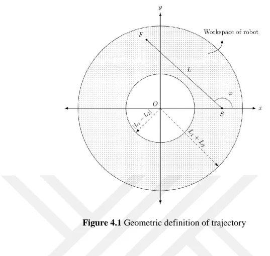
4. DEFINITION OF TASK AND SEARCHING OPTIMAL TRAJECTORY In this work, it is assumed that the task to be executed by the considered planar manipulator is to carry a body of mass 𝑚 in the end effector from a starting point 𝑆 to a final point 𝐹 along a straight line of length 𝐿 in 𝑇 seconds. However, different motion programs, i.e. different velocity and acceleration profiles, can be tested. In all cases, kinematic constraints at point 𝑆 and point 𝐹 will be held same. For a trajectory of certain length 𝐿, once a starting point within the workspace of manipulator, in our study on the x-axis specifically, is chosen the limit values of the direction angle of trajectory 𝜑 are to be obtained. Let the initial value of this angle be 𝜑𝑖𝑛𝑖𝑡. It is found such that the final point of the first trial trajectory stay on the outer boundary of workspace, which is a circle of radius 𝐿1+ 𝐿2. Similarly, the final value of 𝜑, i.e. 𝜑𝑓𝑖𝑛, is obtained considering that the final point of trajectory must stay either on the x-axis or, in the most critical case, on the inner boundary of the workspace, which is a circle of radius |𝐿1− 𝐿2|. Since the workspace is an annular region being symmetric with respect to the x-axis, it is sufficient to confine all the search activity only in the upper semi-plane. Again, for a given length of trajectory, observing the constraint that the final point of trajectory must be on the outer boundary of workspace, the final or minimum value that 𝑥𝑆 can take is calculated. Note that the coordinates of all starting points are in the form of (𝑥𝑆, 0), in other saying, the ordinates of those points will be taken zero without loss of generality. According to what is just mentioned, given the length of trajectory 𝐿 and the abscissa of starting point 𝑥𝑆, 𝑥𝑆𝑓𝑖𝑛 must be determined first. Recall that the initial value of 𝑥𝑆 is same for all trajectory lengths and equal to 𝐿1+ 𝐿2. Then, for a chosen 𝑥𝑆, the limit values of direction angle 𝜑, i.e. 𝜑𝑖𝑛𝑖𝑡 and 𝜑𝑓𝑖𝑛, have to be obtained. Once the initial trial trajectory is defined, for each 𝜑 value which is increased with a certain increment, say 1°, the energy consumption can be computed for each trajectory having the same starting point. Afterwards, among these trial trajectories, the one on which minimal energy is spent is selected as the optimal one. Assuming that this optimal trajectory is fixed in the space, the root point of the manipulator is determined. It is worth noting for the completeness of the study that any point on any radius within the annular region can be taken as starting point 𝑆 during the execution of task.
10
Figure 4.1 Geometric definition of trajectory
Before giving the details of the strategy of searching trial trajectories, it will be explained how to describe a generic trajectory in the following. As is well-known, the equation of a straight line in the xy-plane as follows:
𝑦 = 𝑚𝑥 + 𝑛 (4.1) where 𝑚 ≔ tan 𝜑 =𝑦𝐹− 𝑦𝑆 𝑥𝐹− 𝑥𝑆 𝑛 ≔ 𝑦𝑆𝑥𝐹 − 𝑦𝐹𝑥𝑆 (4.2a) (4.2b) with (𝑥𝑆, 𝑦𝑆) and (𝑥𝐹, 𝑦𝐹) being the coordinates of points 𝑆 and 𝐹 respectively. Defining a unit vector 𝐮 will be useful for future calculations:
𝐮 ≔ cos 𝜑 𝐢 + sin 𝜑 𝐣 (4.3)
The position vector of any point on the trajectory will be as below:
11
where 𝒓𝑆 is the position vector of starting point 𝑆, i.e.
𝐫𝑆 ≔ 𝑥𝑆 𝐢 + 𝑦𝑆 𝐣 (4.5)
and 𝑠 is the distance travelled by the end effector from starting point 𝑆 at any time 𝑡. It is obvious that 𝑠 = 𝑠(𝑡) and the form of relation between 𝑠 and 𝑡 depends on the motion program used, see Figure 4.1.
Now, possible trial trajectories will be discussed. The longest possible trajectory is shown in Figure 4.2. Accordingly, its length is as follows:
𝐿𝑚𝑎𝑥 = 2√(𝐿1+ 𝐿2)2− (𝐿
1− 𝐿2)2 = 2√4 𝐿1𝐿2 = 4√𝐿1𝐿2 (4.6)
Figure 4.2 The longest possible trajectory
The length of trial trajectories cannot be greater than this value. Obviously, there exists only one trajectory whose length is 𝐿𝑚𝑎𝑥. Now, three cases for the interval of 𝑥𝑆 values are distinguished depending upon the length of trajectory:
CASE 1: 𝐿 = 𝐿𝑚𝑎𝑥
12 CASE 2: 𝐿𝑚𝑎𝑥⁄ < 𝐿 < 𝐿2 𝑚𝑎𝑥 𝑥𝑆𝑖𝑛𝑖𝑡 = 𝐿1+ 𝐿2 𝑥𝑆𝑓𝑖𝑛 = √(𝐿1+ 𝐿2) 2+ 𝐿2− 2(𝐿 1+ 𝐿2)𝐿 cos [sin−1( 𝐿1− 𝐿2 𝐿1+ 𝐿2 )] (4.8a) (4.8b) CASE 3: 𝐿 ≤ 𝐿𝑚𝑎𝑥⁄ 2 𝑥𝑆𝑖𝑛𝑖𝑡 = 𝐿1+ 𝐿2 𝑥𝑆𝑓𝑖𝑛 = |𝐿1− 𝐿2| (4.9a) (4.9b) Similar to the above case study, for a certain length of trajectory and given 𝑥𝑆 value, the main and subcases are distinguished to determine the interval of 𝜑 values:
CASE 1: 𝐿 = 𝐿𝑚𝑎𝑥 𝜑𝑖𝑛𝑖𝑡 = 𝜑𝑓𝑖𝑛= 𝜋 − sin−1( 𝐿1− 𝐿2 𝐿1+ 𝐿2) (4.10) CASE 2: 𝐿𝑚𝑎𝑥⁄ ≤ 𝐿 < 𝐿2 𝑚𝑎𝑥 𝜑𝑖𝑛𝑖𝑡 = 𝜋 − cos−1[𝐿 2+ 𝑥 𝑆2− (𝐿1+ 𝐿2)2 2 𝐿 𝑥𝑆 ] 𝜑𝑓𝑖𝑛 = 𝜋 − sin−1( 𝐿1− 𝐿2 𝑥𝑆 ) (4.11a) (4.11b) CASE 3: 2 𝐿2 < 𝐿 < 𝐿𝑚𝑎𝑥⁄ 2 𝜑𝑖𝑛𝑖𝑡 = 𝜋 − cos−1[ 𝐿2+ 𝑥𝑆2− (𝐿1+ 𝐿2)2 2 𝐿 𝑥𝑆 ] 𝛼 ≔ cos−1(𝐿1− 𝐿2 𝑥𝑆 ) 𝜑𝑓𝑖𝑛= { 𝜋 − (𝜋 2− 𝛼) , 𝑥𝑆sin 𝛼 ≤ 𝐿 𝜋 − cos−1[𝐿 2+ 𝑥 𝑆2− (𝐿1− 𝐿2)2 2 𝐿 𝑥𝑆 ] , 𝑥𝑆sin 𝛼 > 𝐿 (4.12a) (4.12b) (4.12c) (4.12d)
13 CASE 4: 𝐿 ≤ 2 𝐿2 Subcase 4.1: 𝐿1+ 𝐿2− 𝑥𝑆 ≥ 𝐿 𝜑𝑖𝑛𝑖𝑡 = 0 𝜑𝑓𝑖𝑛 = { 𝜋, 𝑥𝑆− (𝐿1− 𝐿2) ≥ 𝐿 𝜋 − cos−1[𝐿 2+ 𝑥 𝑆2− (𝐿1− 𝐿2)2 2 𝐿 𝑥𝑆 ] , 𝑥𝑆− (𝐿1− 𝐿2) < 𝐿 (4.13a) (4.13b) (4.13c) Subcase 4.2: 𝐿1+ 𝐿2− 𝑥𝑆 < 𝐿 𝜑𝑖𝑛𝑖𝑡 = 𝜋 − cos−1[𝐿 2 + 𝑥 𝑆2− (𝐿1+ 𝐿2)2 2 𝐿 𝑥𝑆 ] 𝜑𝑓𝑖𝑛 = { 𝜋, 𝑥𝑆− (𝐿1− 𝐿2) ≥ 𝐿 𝜋 − cos−1[𝐿 2+ 𝑥 𝑆2− (𝐿1− 𝐿2)2 2 𝐿 𝑥𝑆 ] , 𝑥𝑆− (𝐿1− 𝐿2) < 𝐿 (4.13d) (4.13e) (4.13f)
The computational procedure will work in the following way:
1. Choose a length of trajectory 𝐿 noting it must be smaller than or equal to 𝐿𝑚𝑎𝑥. 2. From the formulas (4.7) to (4.9), use the appropriate one for the chosen length,
and find 𝑥𝑆𝑓𝑖𝑛.
3. Determine that the interval of 𝑥𝑆 will be divided to how many subinterval. The step size ∆𝑥 between successive starting points can be found dividing the interval |𝑥𝑆𝑓𝑖𝑛− 𝑥𝑆𝑖𝑛𝑖𝑡| by 𝑛𝑥𝑆. The number of starting points to be used during computation is then (|𝑥𝑆𝑓𝑖𝑛 − 𝑥𝑆𝑖𝑛𝑖𝑡| ∆𝑥⁄ ) + 1.
4. For a starting point chosen, use the appropriate one between formulas (4.10) to (4.13) to obtain then interval of direction angle 𝜑 for the starting point chosen and the given length.
5. Find the number of straight-lines in the bunch of trial trajectories dividing the interval |𝜑𝑓𝑖𝑛− 𝜑𝑖𝑛𝑖𝑡| by ∆𝜑. Hence, the number of these points equals to (|𝜑𝑓𝑖𝑛− 𝜑𝑖𝑛𝑖𝑡| ∆𝜑⁄ ) + 1.
6. For each of trial trajectories, compute the energy consumption and store them. 7. Repeat the procedure for other starting points.
14
9. Plot all relevant graphics, e.g. displacement, angular velocities and accelerations, actuator torques, energy consumption curves for the energy-optimal trajectory.
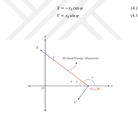
Usually in the practice, repositioning of a production or assembly line is quite difficult. If a robot arm is to be introduced into such a production line, then the only alternative is to find such an appropriate location for the robot that the energy consumption during that pre-defined operation be minimal. In this case, especially for the trajectory discussed here, a new coordinate system is defined as shown in Figure 4.3 to fix the location of the robot with respect to the trajectory, or in some sense, production line. In this new coordinate system, the position of the root of robot arm can be obtained just using the starting point 𝑥𝑆 and the orientation angle 𝜑 of the energy-optimal trajectory. Consequently, these coordinates are obtained as follows:
𝑋 = −𝑥𝑆cos 𝜑 𝑌 = 𝑥𝑆sin 𝜑
(4.14a) (4.14b)
15
5. KINEMATIC CONSTRAINTS, VELOCITY AND ACCELERATION FUNCTIONS
The kinematic constraints are given below:
𝑎𝑡 𝑡 = 0, 𝑠(0) = 0, 𝑠̇(0) = 0, 𝑠̈(0) = 0 (5.1a) 𝑎𝑡 𝑡 = 𝑇, 𝑠(𝑇) = 𝐿, 𝑠̇(𝑇) = 0, 𝑠̈(𝑇) = 0 (5.1b) where 𝑠, 𝑠̇ and 𝑠̈ show the displacement on the trajectory, its first time derivative and its second time derivation respectively. Kinematic constraints are given by equations (5.1) imply that the motion at the beginning and at the end must be impact- and jerk-free. In this work, two different displacement functions will be used. One of them is a cycloidal displacement function while the other is a 3-4-5 polynomial. Consequently, the displacement, velocity and acceleration functions are as follows: Cycloidal Motion: 𝑠(𝑡) = 𝐿 (𝑡 𝑇− 1 2𝜋sin 2𝜋𝑡 𝑇 ) 𝑠̇(𝑡) =𝐿 𝑇(1 − cos 2𝜋𝑡 𝑇 ) 𝑠̈(𝑡) =2𝜋𝐿 𝑇2 sin 2𝜋𝑡 𝑇 (5.2a) (5.2b) (5.2c) 3-4-5 Polynomial Motion: 𝑠(𝑡) = 𝐿 [6 (𝑡 𝑇) 5 − 15 (𝑡 𝑇) 4 + 10 (𝑡 𝑇) 3 ] 𝑠̇(𝑡) =𝐿 𝑇[30 ( 𝑡 𝑇) 4 − 60 (𝑡 𝑇) 3 + 30 (𝑡 𝑇) 2 ] 𝑠̈(𝑡) = 𝐿 𝑇2[120 ( 𝑡 𝑇) 3 − 180 (𝑡 𝑇) 2 + 60 (𝑡 𝑇) 1 ] (5.3a) (5.3b) (5.3c)
16 6. EQUATIONS OF MOTION
This section is devoted to deriving equations of motion by using Lagrangian approach. As is well-known, the first step of this approach is to obtain kinetic and potential energy terms of the system. Hence the linear velocities of certain system points like center of gravities and joints. These points are 𝐺1, 𝐴1, 𝐺2 and 𝐵 (see Figure 3.1). Velocity of point 𝐺1:
𝐯𝐺1 = 𝜃̇1 𝐤 𝑥 (𝑟𝐺1cos 𝜃1𝐢 + 𝑟𝐺1sin 𝜃1𝐣)
= −𝑟𝐺1sin 𝜃1𝜃̇1 𝐢 + 𝑟𝐺1cos 𝜃1𝜃̇1 𝐣 (6.1) where 𝑟𝐺1 = 𝑂𝐺̅̅̅̅̅ and 𝜃̇1 1𝐤 is the angular velocity of link 1. From (6.1) one obtains:
𝐯𝐺21 = 𝐯𝐺1 ⋅ 𝐯𝐺1 = 𝑟𝐺21 𝜃̇12 (6.2) Velocity of point 𝐴: 𝐯𝐴 = 𝜃̇1 𝐤 𝑥 (𝐿1cos 𝜃1𝐢 + 𝐿1sin 𝜃1 𝐣) = −𝐿1sin 𝜃1𝜃̇1 𝐢 + 𝐿1cos 𝜃1𝜃̇1 𝐣 (6.3) From (6.3) we find: 𝐯𝐴2 = 𝐯𝐴⋅ 𝐯𝐴 = 𝐿21 𝜃̇12 (6.4) Velocity of point 𝐺2: 𝐯𝐺2 = 𝐯𝐴 + 𝐯𝐺2⁄𝐴 𝐯𝐺2⁄𝐴 = 𝜃̇2 𝐤 𝑥 (𝑟𝐺2cos 𝜃2𝐢 + 𝑟𝐺2sin 𝜃2𝐣) = −𝑟𝐺2sin 𝜃2𝜃̇2 𝐢 + 𝑟𝐺2cos 𝜃2𝜃̇2 𝐣 𝐯𝐺2 = −(𝐿1sin 𝜃1𝜃̇1+ 𝑟𝐺2sin 𝜃2𝜃̇2) 𝐢 + (𝐿1cos 𝜃1𝜃̇1+ 𝑟𝐺2cos 𝜃2𝜃̇2) 𝐣 (6.5) (6.6) (6.7)
Similarly, from (6.7) one finds: 𝐯𝐺22 = 𝐯𝐺2⋅ 𝐯𝐺2 = 𝐿1
2 𝜃̇
12+ 𝑟𝐺2 2 𝜃̇
17 Velocity of point 𝐵: 𝐯𝐵= 𝐯𝐴+ 𝐯𝐵 𝐴⁄ 𝐯𝐵 𝐴⁄ = 𝜃̇2 𝐤 𝑥 (𝐿2cos 𝜃2𝐢 + 𝐿2sin 𝜃2𝐣) = −𝐿2sin 𝜃2𝜃̇2 𝐢 + 𝐿2cos 𝜃2𝜃̇2 𝐣 𝐯𝐵= −(𝐿1sin 𝜃1𝜃̇1+ 𝐿2sin 𝜃2𝜃̇2) 𝐢 + (𝐿1cos 𝜃1𝜃̇1+ 𝐿2cos 𝜃2𝜃̇2) 𝐣 (6.9) (6.10) (6.11)
Taking square of |𝐯𝐵| yields:
𝐯𝐵2 = 𝐯𝐵⋅ 𝐯𝐵 = 𝐿21 𝜃̇12+ 𝐿22 𝜃̇22+ 2 𝐿1 𝐿2cos(𝜃2− 𝜃1) 𝜃̇1𝜃̇2 (6.12) Kinetic energy of link 1:
𝑇1 =1 2𝐼𝐺1𝜃̇1 2+1 2𝑚1 𝑣𝐺1 2 =1 2𝐼𝐺1𝜃̇1 2+1 2𝑚1 𝑟𝐺1 2 𝜃̇ 12 =1 2(𝐼𝐺1+ 𝑚1 𝑟𝐺1 2) 𝜃̇ 12 (6.13)
According to the parallel-axes theorem we can define: 𝐼1,𝑂 ≔ 𝐼𝐺1 + 𝑚1 𝑟𝐺1
2 (6.14)
where 𝐼1,𝑂 is the mass moment of inertia of link 1 about the axis through the joint at 𝑂.
Kinetic energy of link 2: 𝑇2 = 1 2𝐼𝐺2𝜃̇2 2+1 2𝑚2 𝑣𝐺2 2 = 1 2𝐼𝐺2𝜃̇2 2+1 2𝑚2[𝐿1 2 𝜃̇ 12+ 𝑟𝐺2 2 𝜃̇ 22] + 2 𝐿1 𝑟𝐺2cos(𝜃2− 𝜃1) 𝜃̇1𝜃̇2 (6.15) Here we also define:
𝐼2,𝐴≔ 𝐼𝐺2+ 𝑚2 𝑟𝐺22 (6.16) where 𝐼2,𝐴 is the mass moment of inertia of link 2 about the axis through the joint at 𝐴.
18
Consequently, equation (6.15) can be written as follows: 𝐼2 = 1 2𝐼2,𝐴 𝜃̇2 2+1 2𝑚2 𝐿1 2 𝜃̇ 12+ 𝑚2 𝐿1 𝑟𝐺2cos(𝜃2− 𝜃1) 𝜃̇1𝜃̇2 (6.17) Kinetic energy of the object of mass 𝑚 carried with end effector:
𝑇𝑚 =1 2𝑚 𝑣𝐵 2 =1 2𝑚[𝐿1 2 𝜃̇ 12 + 𝐿22 𝜃̇22] + 𝑚 𝐿1 𝐿2cos(𝜃2− 𝜃1) 𝜃̇1𝜃̇2 (6.18) Virtual works of actuator torques:
Actuator 1: 𝛿𝑊1 = 𝐌𝟏⋅ 𝛅𝛉𝟏 = 𝑀1 𝐤 ⋅ 𝛿𝜃1 𝐤 = 𝑀1 𝛿𝜃1 (6.19) Actuator 2: 𝛿𝑊2 = 𝐌𝟐⋅ (𝛅𝛉𝟐− 𝛅𝛉𝟏) = 𝑀2 𝐤 ⋅ (𝛿𝜃2 𝐤 − 𝛿𝜃1 𝐤) = 𝑀2 𝛿𝜃2− 𝑀2 𝛿𝜃1 (6.20)
Total virtual work:
𝛿𝑊 = 𝛿𝑊1+ 𝛿𝑊2
= (𝑀1− 𝑀2) 𝛿𝜃1+ 𝑀2𝛿𝜃2 (6.21) Total kinetic energy:
𝑇 = 𝑇1+ 𝑇2+ 𝑇𝑚 =1 2𝐼1,𝑂 𝜃̇1 2+1 2𝐼2,𝐴 𝜃̇2 2+1 2𝑚2 𝐿1 2 𝜃̇ 12 + 𝑚2 𝐿1 𝑟𝐺2cos(𝜃2− 𝜃1) 𝜃̇1𝜃̇2 +1 2𝑚[𝐿1 2 𝜃̇ 12+ 𝐿22 𝜃̇22] + 𝑚 𝐿1𝐿2cos(𝜃2 − 𝜃1) 𝜃̇1𝜃̇2 (6.22) or rearranging we find: 𝑇 =1 2(𝐼1,𝑂+ 𝑚2𝐿1 2 + 𝑚𝐿 1 2) 𝜃̇ 12+ 1 2(𝐼2,𝐴+ 𝑚𝐿2 2) 𝜃̇ 22 + (𝑚2𝐿1𝑟𝐺2 + 𝑚 𝐿1𝐿2) cos(𝜃2− 𝜃1) 𝜃̇1𝜃̇2 (6.23)
19 Equation of Motion of Link 1:
According to the Lagrangian mechanics, the equation of motion is given by the following formula: d d𝑡( 𝜕𝑇 𝜕𝜃̇1 ) − 𝜕𝑇 𝜕𝜃1 = 𝑄1 (6.24) where 𝑄1 ≔ 𝑀1 − 𝑀2 (6.25)
Let us calculate the terms on the left side of equation (6.24): 𝜕𝑇 𝜕𝜃̇1 = [𝐼1,𝑂+ (𝑚2+ 𝑚) 𝐿21] 𝜃̇1+ (𝑚2𝐿1𝑟𝐺2+ 𝑚 𝐿1𝐿2) cos(𝜃2− 𝜃1) 𝜃̇2 (6.26) Therefore, d d𝑡( 𝜕𝑇 𝜕𝜃̇1) = [𝐼1,𝑂+ (𝑚2+ 𝑚) 𝐿1 2] 𝜃̈ 1 − (𝑚2𝐿1𝑟𝐺2 + 𝑚 𝐿1𝐿2) sin(𝜃2 − 𝜃1) 𝜃̇2 2 + (𝑚2𝐿1𝑟𝐺2 + 𝑚 𝐿1𝐿2) cos(𝜃2− 𝜃1) 𝜃̈2 + (𝑚2𝐿1𝑟𝐺2 + 𝑚 𝐿1𝐿2) sin(𝜃2 − 𝜃1) 𝜃̇1𝜃̇2 (6.27) and 𝜕𝑇 𝜕𝜃1 = −(𝑚2𝐿1𝑟𝐺2+ 𝑚 𝐿1𝐿2) sin(𝜃2− 𝜃1) (−1) 𝜃̇1𝜃̇2 = (𝑚2𝐿1𝑟𝐺2 + 𝑚 𝐿1𝐿2) sin(𝜃2− 𝜃1) 𝜃̇1𝜃̇2 (6.28)
Substituting equations (6.25), (6.27) and (6.28) in equation (6.24) yields 𝑀1− 𝑀2 = [𝐼1,𝑂+ (𝑚2+ 𝑚) 𝐿21] 𝜃̈1
+ (𝑚2𝐿1𝑟𝐺2+ 𝑚 𝐿1𝐿2) cos(𝜃2− 𝜃1) 𝜃̈2 − (𝑚2𝐿1𝑟𝐺2+ 𝑚 𝐿1𝐿2) sin(𝜃2− 𝜃1) 𝜃̇2
2
20 Equation of Motion of Link 2:
The Lagrangian form of the equation of motion for link 2 is as follows: d d𝑡( 𝜕𝑇 𝜕𝜃̇2 ) − 𝜕𝑇 𝜕𝜃2 = 𝑄2 (6.30) where 𝑄2 ≔ 𝑀2 (6.31)
Let us calculate the terms on the left side of equation (6.30): 𝜕𝑇 𝜕𝜃̇2 = (𝐼2,𝐴+ 𝑚 𝐿2 2) 𝜃̇ 2+ (𝑚2𝐿1𝑟𝐺2 + 𝑚 𝐿1𝐿2) cos(𝜃2− 𝜃1) 𝜃̇1 (6.32) Therefore d d𝑡( 𝜕𝑇 𝜕𝜃̇2) = (𝐼2,𝐴+ 𝑚 𝐿2 2) 𝜃̈ 2 − (𝑚2𝐿1𝑟𝐺2 + 𝑚 𝐿1𝐿2) sin(𝜃2− 𝜃1) (𝜃̇2− 𝜃̇1) 𝜃̇1 + (𝑚2𝐿1𝑟𝐺2 + 𝑚 𝐿1𝐿2) cos(𝜃2− 𝜃1) 𝜃̈1 = (𝐼2,𝐴+ 𝑚 𝐿22) 𝜃̈ 2 + (𝑚2𝐿1𝑟𝐺2+ 𝑚 𝐿1𝐿2) sin(𝜃2− 𝜃1) 𝜃̇1 2 + (𝑚2𝐿1𝑟𝐺2 + 𝑚 𝐿1𝐿2) cos(𝜃2− 𝜃1) 𝜃̈1 − (𝑚2𝐿1𝑟𝐺2 + 𝑚 𝐿1𝐿2) sin(𝜃2− 𝜃1) 𝜃̇1𝜃̈2 (6.33) and 𝜕𝑇 𝜕𝜃2 = −(𝑚2𝐿1𝑟𝐺2+ 𝑚 𝐿1𝐿2) sin(𝜃2− 𝜃1) 𝜃̇1𝜃̇2 (6.34) Substituting equations (6.31), (6.33) and (6.34) in (6.30), one obtains the following:
𝑀2 = (𝐼2,𝐴+ 𝑚 𝐿22) 𝜃̈2+ (𝑚2𝐿1𝑟𝐺2 + 𝑚 𝐿1𝐿2) cos(𝜃2− 𝜃1) 𝜃̈1 + (𝑚2𝐿1𝑟𝐺2 + 𝑚 𝐿1𝐿2) sin(𝜃2 − 𝜃1) 𝜃̇1
21
7. SOLVING EQUATION OF MOTION FOR ACTUATOR TORQUES The torque of actuator 1, 𝑀1, is obtained by adding equations (6.29) and (6.35) as follows: 𝑀1 = [𝐼1,𝑂+ (𝑚2+ 𝑚) 𝐿21+ (𝑚2𝐿1𝑟𝐺2+ 𝑚 𝐿1𝐿2) cos(𝜃2− 𝜃1)]𝜃̈1 + [𝐼2,𝐴+ 𝑚 𝐿22 + (𝑚2𝐿1𝑟𝐺2+ 𝑚 𝐿1𝐿2) cos(𝜃2− 𝜃1)]𝜃̈2 + (𝑚2𝐿1𝑟𝐺2 + 𝑚 𝐿1𝐿2) sin(𝜃2− 𝜃1) 𝜃̇12 − (𝑚2𝐿1𝑟𝐺2 + 𝑚 𝐿1𝐿2) sin(𝜃2− 𝜃1) 𝜃̇2 2 (7.1)
Similarly, the torque of actuator 2, 𝑀2, is found by subtracting equation (6.29) from (6.35) and dividing each side of the resulting equation by 2 as follows:
𝑀2 = 1 2{[(𝑚2𝐿1𝑟𝐺2+ 𝑚 𝐿1𝐿2) cos(𝜃2− 𝜃1) − 𝐼1,𝑂− (𝑚2+ 𝑚) 𝐿1 2]𝜃̈ 1 + [𝐼2,𝐴+ 𝑚 𝐿22− (𝑚2𝐿1𝑟𝐺2+ 𝑚 𝐿1𝐿2) cos(𝜃2− 𝜃1)]𝜃̈2 + (𝑚2𝐿1𝑟𝐺2 + 𝑚 𝐿1𝐿2) sin(𝜃2 − 𝜃1) 𝜃̇12 + (𝑚2𝐿1𝑟𝐺2 + 𝑚 𝐿1𝐿2) sin(𝜃2 − 𝜃1) 𝜃̇22} (7.2)
22
8. CALCULATION OF ENERGY CONSUMPTION
The energy consumed during a complete operation is given by the following formula:
𝐸 = ∫ |𝐌𝟏⋅ d 𝛉𝟏| + |𝐌𝟐⋅ (d 𝛉𝟐− d 𝛉𝟏)| 𝒓𝑭
𝒓𝑺
(8.1)
where 𝐫𝐒 and 𝐫𝐅 denote the position vectors of the starting and final points of the trajectory, respectively. Explicitly expressed, these vectors are as follows:
𝐫𝐒 = 𝑥𝑆 𝐢 + 𝑦𝑆 𝐣 𝐫𝐅 = 𝑥𝐹 𝐢 + 𝑦𝐹 𝐣
(8.2a) (8.2b) It should be noted that the following requirements are to be satisfied:
𝑥𝑆2+ 𝑦𝑆2 ≤ (𝐿1+ 𝐿2)𝟐 𝑥𝐹2+ 𝑦𝐹2 ≤ (𝐿1+ 𝐿2)𝟐
(8.3a) (8.3b) Furthermore, the following relationship exists:
𝐫𝐅 = 𝐫𝐒+ 𝐿 𝐮 (8.4)
In terms of the components of position vectors 𝐫𝐒 and 𝐫𝐅, equation (8.4) can be written as below:
𝑥𝐹 = 𝑥𝑆+ 𝐿 cos 𝜙 𝑦𝐹 = 𝑦𝑆+ 𝐿 sin 𝜙
(8.5a) (8.5b) The integral (8.1) can be calculated numerically after discretization of it.
23 9. NUMERICAL EXAMPLES
To carry out the computational procedure explained in Chapters 4-8, a MATLAB code was developed. This chapter is devoted to some numerical examples which help understand the solution approach presented in this work. It is assumed that actuators provide torques needed every time in the examples. Control dynamics is not considered. Masses and inertia moments of actuators are also omitted for simplicity. For all numerical examples, the manipulator is assumed to have the following physical parameters: Link 1: 𝐿1 = 0.4 𝑚 𝑚1 = 4 𝑘𝑔 𝑟𝐺1 = 0.5 𝐿1 = 0.2 𝑚 𝐼𝐺1 = 𝑚1 𝐿21 12⁄ = 0.0533 𝑘𝑔-𝑚2 𝐼1,𝑂= 𝐼𝐺1 + 𝑚1 𝑟𝐺1 2 = 0.2133 𝑘𝑔-𝑚2 Link 2: 𝐿2 = 0.2 𝑚 𝑚2 = 2 𝑘𝑔 𝑟𝐺2 = 0.5 𝐿2 = 0.1 𝑚 𝐼𝐺2 = 𝑚2 𝐿2 2 12⁄ = 0.00167 𝑘𝑔-𝑚2 Payload: 𝑚 = 1 𝑘𝑔
With these lengths of links, the length of longest possible trajectory becomes 𝐿𝑚𝑎𝑥 = 4√𝐿1𝐿2 = 4√0.4 × 0.2 = 1.1314 𝑚
24
In this chapter, five examples will be given for the following cases: 1. 𝐿 = 𝐿𝑚𝑎𝑥
2. 𝐿𝑚𝑎𝑥⁄ < 𝐿 < 𝐿2 𝑚𝑎𝑥 3. 𝐿 = 𝐿𝑚𝑎𝑥⁄ 2
4. 2 𝐿2 < 𝐿 < 𝐿𝑚𝑎𝑥⁄ 2 5. 𝐿 ≤ 2 𝐿2
For each case, one numerical example is given. In each example, minimum values for cycloidal and 3-4-5 polynomial motion programs are calculated. Only figures of cycloidal motion program is provided since figures are very similar in both motion programs.
Example 1: (𝐿 = 𝐿𝑚𝑎𝑥)
Let 𝐿 = 𝐿𝑚𝑎𝑥 and 𝑇 = 1 second. As is known, there is only one solution to this case. Computer results are as follows:
𝑥𝑆𝑖𝑛𝑖𝑡 = 𝑥𝑆𝑓𝑖𝑛 = 𝐿1+ 𝐿2 = 0.6 𝑚 𝜑𝑖𝑛𝑖𝑡 = 𝜑𝑓𝑖𝑛 = 160.53°
These values are common to the first and second configurations. Minimum energy consumptions for the first configuration:
𝑚𝑖𝑛(𝐸𝐶1) = 389.05 𝑗𝑜𝑢𝑙𝑒𝑠 (Cycloidal motion program)
𝑚𝑖𝑛(𝐸𝐶1) = 344.77 𝑗𝑜𝑢𝑙𝑒𝑠 (3-4-5 polynomial motion program) Minimum energy consumptions for the second configuration:
𝑚𝑖𝑛(𝐸𝐶2) = 32.61 𝑗𝑜𝑢𝑙𝑒𝑠 (Cycloidal motion program)
𝑚𝑖𝑛(𝐸𝐶2) = 29.37 𝑗𝑜𝑢𝑙𝑒𝑠 (3-4-5 polynomial motion program)
It is seen that the second configuration leads to the less consumption of energy for both motion programs. For each configuration of cycloidal motion program, how position coordinates, angular velocities, angular accelerations, actuator torques and actuator powers change versus time are shown in Figures 9.1-9.5 respectively.
25
Figure 9.1 Position angles of links in Example 1 (𝜃11 and 𝜃21 are position angles of link 1 and link 2 for the first configuration while 𝜃12 and 𝜃22 are position angles of link 1 and link 2 for the second configuration)
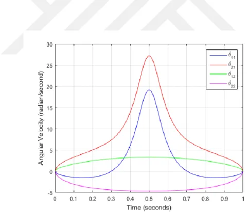
Figure 9.2 Angular velocities of links in Example 1 (𝜃̇11 and 𝜃̇21 are angular velocities of link 1 and link 2 for the first configuration while 𝜃̇12 and 𝜃̇22 are angular velocities of link 1 and link 2 for the second configuration)
26
Figure 9.3 Angular accelerations of links in Example 1 (𝜃̈11 and 𝜃̈21 are angular accelerations of link 1 and link 2 for the first configuration while 𝜃̈12 and 𝜃̈22 are angular accelerations of link 1 and link 2 for the second configuration)
Figure 9.4 Actuator torques of links in Example 1 (𝑀11 and 𝑀21 are actuator torques of link 1 and link 2 for the first configuration while 𝑀12 and 𝑀22 are actuator torques of link 1 and link 2 for the second configuration)
27
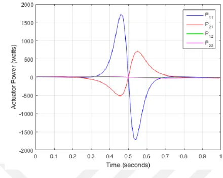
Figure 9.5 Actuator powers of links in Example 1 (𝑃11 and 𝑃21 are actuator powers of link 1 and link 2 for the first configuration while 𝑃12 and 𝑃22 are actuator powers of link 1 and link 2 for the second configuration)
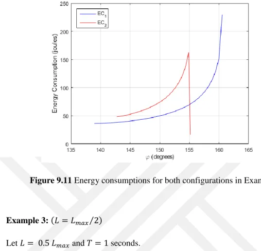
Example 2: (𝐿𝑚𝑎𝑥⁄ < 𝐿 < 𝐿2 𝑚𝑎𝑥) Let 𝐿 = 0.8 𝐿𝑚𝑎𝑥 and 𝑇 = 1 seconds.
Minimum energy consumptions for the first configuration:
𝑚𝑖𝑛(𝐸𝐶1) = 36.24 𝑗𝑜𝑢𝑙𝑒𝑠 (Cycloidal motion program)
𝑚𝑖𝑛(𝐸𝐶1) = 32.96 𝑗𝑜𝑢𝑙𝑒𝑠 (3-4-5 polynomial motion program)
For both motion programs, the abscissa of starting point and the direction angle of the optimal trajectories are same, hence, these two trajectories are identical:
𝑥𝑆,1 = 𝐿1+ 𝐿2 = 0.6 𝑚 𝜑1 = 𝜑𝑖𝑛𝑖𝑡 = 138.96°
Minimum energy consumptions for the second configuration: 𝑚𝑖𝑛(𝐸𝐶2) = 16.54 𝑗𝑜𝑢𝑙𝑒𝑠 (Cycloidal motion program)
28
Again, for both motion programs there exists only one trajectory. The abscissa of starting point and the direction angle of that trajectory are as follows:
𝑥𝑆,2 = 0.4764 𝑚 𝜑2 = 155.18°
Also for this case, the second configuration should be preferred regarding energy consumption.
Figures 9.6-9.10 depict the changes of positions, velocities, accelerations, torques and powers with respect to time. In Figure 9.11, we see how energy consumptions vary over direction angles.
Figure 9.6 Position angles of links in Example 2 (𝜃11 and 𝜃21 are position angles of link 1 and link 2 for the first configuration while 𝜃12 and 𝜃22 are position angles of link 1 and link 2 for the second configuration)
29
Figure 9.7 Angular velocities of links in Example 2 (𝜃̇11 and 𝜃̇21 are angular velocities of link 1 and link 2 for the first configuration while 𝜃̇12 and 𝜃̇22 are angular velocities of link 1 and link 2 for the second configuration)
Figure 9.8 Angular accelerations of links in Example 2 (𝜃̈11 and 𝜃̈21 are angular accelerations of link 1 and link 2 for the first configuration while 𝜃̈12 and 𝜃̈22 are angular accelerations of link 1 and link 2 for the second configuration)
30
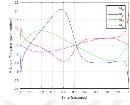
Figure 9.9 Actuator torques of links in Example 2 (𝑀11 and 𝑀21 are actuator torques of link 1 and link 2 for the first configuration while 𝑀12 and 𝑀22 are actuator torques of link 1 and link 2 for the second configuration)
Figure 9.10 Actuator powers of links in Example 2 (𝑃11 and 𝑃21 are actuator powers of link 1 and link 2 for the first configuration while 𝑃12 and 𝑃22 are actuator powers of link 1 and link 2 for the second configuration)
31
Figure 9.11 Energy consumptions for both configurations in Example 2
Example 3: (𝐿 = 𝐿𝑚𝑎𝑥⁄ ) 2
Let 𝐿 = 0.5 𝐿𝑚𝑎𝑥 and 𝑇 = 1 seconds.
Minimum energy consumptions for the first configuration:
𝑚𝑖𝑛(𝐸𝐶1) = 9.58 𝑗𝑜𝑢𝑙𝑒𝑠 (Cycloidal motion program)
𝑚𝑖𝑛(𝐸𝐶1) = 8.48 𝑗𝑜𝑢𝑙𝑒𝑠 (3-4-5 polynomial motion program)
For both motion programs, energy-optimal trajectories are identical. The starting point and direction angle related to this trajectory are:
𝑥𝑆,1 = 0.52 𝑚 𝜑1 = 121.92°
Minimum energy consumptions for the second configuration: 𝑚𝑖𝑛(𝐸𝐶2) = 5.53 𝑗𝑜𝑢𝑙𝑒𝑠 (Cycloidal motion program)
32
Again, there is one energy-optimal trajectory common to both motion programs. Characteristic parameters related to this trajectory are:
𝑥𝑆,2 = 0.36 𝑚 𝜑2 = 146.25°
Figures 9.12-9.17 show the change of kinematic and kinetic parameters with time or direction angles.
Figure 9.12 Position angles of links in Example 3 (𝜃11 and 𝜃21 are position angles of link 1 and link 2 for the first configuration while 𝜃12 and 𝜃22 are position angles of link 1 and link 2 for the second configuration)
33
Figure 9.13 Angular velocities of links in Example 3 (𝜃̇11 and 𝜃̇21 are angular velocities of link 1 and link 2 for the first configuration while 𝜃̇12 and 𝜃̇22 are angular velocities of link 1 and link 2 for the second configuration)
Figure 9.14 Angular accelerations of links in Example 3 (𝜃̈11 and 𝜃̈21 are angular accelerations of link 1 and link 2 for the first configuration as 𝜃̈12 and 𝜃̈22 are angular accelerations of link 1 and link 2 for the second configuration)
34
Figure 9.15 Actuator torques of links in Example 3 (𝑀11 and 𝑀21 are actuator torques of link 1 and link 2 for the first configuration while 𝑀12 and 𝑀22 are actuator torques of link 1 and link 2 for the second configuration)
Figure 9.16 Actuator powers of links in Example 3 (𝑃11 and 𝑃21 are actuator powers of link 1 and link 2 for the first configuration while 𝑃12 and 𝑃22 are actuator powers of link 1 and link 2 for the second configuration)
35
Figure 9.17 Energy consumptions for both configurations in Example 3
Example 4: (2 𝐿2 < 𝐿 < 𝐿𝑚𝑎𝑥⁄ ) 2 Let 𝐿 = 0.4 𝐿𝑚𝑎𝑥 and 𝑇 = 1 seconds.
Minimum energy consumptions for the first configuration:
𝑚𝑖𝑛(𝐸𝐶1) = 5.23 𝑗𝑜𝑢𝑙𝑒𝑠 (Cycloidal motion program)
𝑚𝑖𝑛(𝐸𝐶1) = 4.63 𝑗𝑜𝑢𝑙𝑒𝑠 (3-4-5 polynomial motion program)
As in previous cases, energy-optimal trajectories are identical for both motion programs. The starting point and direction angle related to this trajectory are:
𝑥𝑆,1 = 0.52 𝑚 𝜑1 = 130.89°
Minimum energy consumptions for the second configuration: 𝑚𝑖𝑛(𝐸𝐶2) = 3.44 𝑗𝑜𝑢𝑙𝑒𝑠 (Cycloidal motion program)
36
The common energy-optimal trajectory has the following starting point and direction angle:
𝑥𝑆,2 = 0.28 𝑚 𝜑2 = 134.42°
The second configuration seems to be more economical also for this case. The relevant graphics are Figures 9.18-9.23.
Figure 9.18 Position angles of links in Example 4 (𝜃11 and 𝜃21 are position angles of link 1 and link 2 for the first configuration while 𝜃12 and 𝜃22 are position angles of link 1 and link 2 for the second configuration)
37
Figure 9.19 Angular velocities of links in Example 4 (𝜃̇11 and 𝜃̇21 are angular velocities of link 1 and link 2 for the first configuration while 𝜃̇12 and 𝜃̇22 are angular velocities of link 1 and link 2 for the second configuration)
Figure 9.20 Angular accelerations of links in Example 4 (𝜃̈11 and 𝜃̈21 are angular accelerations of link 1 and link 2 for the first configuration as 𝜃̈12 and 𝜃̈22 are angular accelerations of link 1 and link 2 for the second configuration)
38
Figure 9.21 Actuator torques of links in Example 4 (𝑀11 and 𝑀21 are actuator torques of link 1 and link 2 for the first configuration while 𝑀12 and 𝑀22 are actuator torques of link 1 and link 2 for the second configuration)
Figure 9.22 Actuator powers of links in Example 4 (𝑃11 and 𝑃21 are actuator powers of link 1 and link 2 for the first configuration while 𝑃12 and 𝑃22 are actuator powers of link 1 and link 2 for the second configuration)
39
Figure 9.23 Energy consumptions for both configurations in Example 4
Example 5: (𝐿 ≤ 2 𝐿2)
Let 𝐿 = 0.2 𝐿𝑚𝑎𝑥 and 𝑇 = 1 seconds.
Minimum energy consumptions for the first configuration:
𝑚𝑖𝑛(𝐸𝐶1) = 0.83 𝑗𝑜𝑢𝑙𝑒𝑠 (Cycloidal motion program)
𝑚𝑖𝑛(𝐸𝐶1) = 0.74 𝑗𝑜𝑢𝑙𝑒𝑠 (3-4-5 polynomial motion program) The common energy-optimal trajectory has the following characteristic values: 𝑥𝑆,1 = 0.52 𝑚
𝜑1 = 130.3°
Minimum energy consumptions for the second configuration: 𝑚𝑖𝑛(𝐸𝐶2) = 0.59 𝑗𝑜𝑢𝑙𝑒𝑠 (Cycloidal motion program)
40
For this configuration, the starting point’s abscissa and the direction angle of the trajectory are as follows:
𝑥𝑆,2 = 0.44 𝑚 𝜑2 = 67.19°
The relevant graphics are presented in Figures 9.24-9.29.
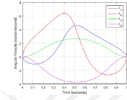
Figure 9.24 Position angles of links in Example 5 (𝜃11 and 𝜃21 are position angles of link 1 and link 2 for the first configuration while 𝜃12 and 𝜃22 are position angles of link 1 and link 2 for the second configuration)
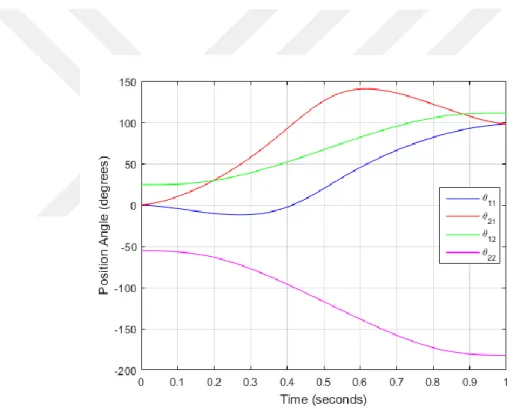
41
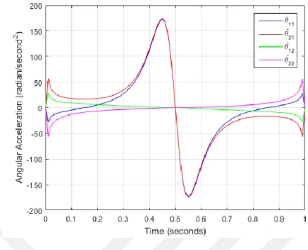
Figure 9.25 Angular velocities of links in Example 5 (𝜃̇11 and 𝜃̇21 are angular velocities of link 1 and link 2 for the first configuration while 𝜃̇12 and 𝜃̇22 are angular velocities of link 1 and link 2 for the second configuration)
Figure 9.26 Angular accelerations of links in Example 5 (𝜃̈11 and 𝜃̈21 are angular accelerations of link 1 and link 2 for the first configuration as 𝜃̈12 and 𝜃̈22 are angular accelerations of link 1 and link 2 for the second configuration)