Formal GARCH performance in a computable dynamic general equilibrium framework

. r £. Лг

;. , і-'·· г - ^ .. Jv-z/V İat- - - , с : · - ν . ' / , · : > ^ 4 · Γ ^ . < - ; . ^ · : : · ν · · ν - - ^ ',

FORMAL GARCH PERFORMANCE IN A COMPUTABLE

DYNAMIC GENERAL EQUILIBRIUM FRAMEWORK

A THESIS

Submitted to the Faculty of Management and the Graduate School of Business Administration

of Bilkent University

in Partial Fulflilment of the Requirements For the Degree of

Master of Science in Business Administration

ALi BORA YiGiTBA$IOGLU ANKARA, AUGUST 1998

1 certify that 1 have read this thesis and in my opinion it is fully adequate, in scope and in quality, as a thesis for the degree of Master o f Science in Business Administration.

Assist. Prof. Aslihan Salih

I certify that I have read this thesis and in my opinion it is fully adequate, in scope and in quality, as a thesis for the degree of Master of Science in Business Administration.

Assoc. Prof. Kursat Aydogan

I certify that I have read this thesis and in my opinion it is fully adequate, in scope and in quality, as a thesis for the degree of Master of Science in Business Administration.

Assist. Prof. Levent Akdeniz

I

НИ

&053764

ABSTRACT

FORMAL GARCH PERFORMANCE IN A COMPUTABLE

DYNAMIC GENERAL EQUILIBRIUM FRAMEWORK

ALİ BORA YİĞİTBAŞIOĞLU Master of Science in Business Administration

Supen isor: Assist. Prof. Aslihan Salih August, 1998

This study uses a Computable Dynamic General Equilibrium setting based on Brock’s (1979, 1982) intertemporal growth and asset pricing models and applies this framework as a formal test to study the out-of-sample forecast performance of Bollerslev’s (1986) GARCH (1,1) Classical Historical Volatility forecasts. The solution to Brock’s growth model reflects the utility maximizing behavior of the consumer and profit maximizing behavior of producers, and is a framework that has recorded some remarkable successes in mirroring the real economy. All existing studies have used a sample realized variance in the forecast horizon to test the out-of- sample performance of conditional variance forecasting models. The realized variance is simply an approximation to the true distribution of variance in the forecast horizon, and is often an unfair benchmark of performance. Simulation of Brock’s model enables one to obtain the true distribution of asset returns and their variance at all times. The true distribution reflects all the possible states of a simulated economy, which is shown to mimic all the properties observed in empirical financial data. This framework affords the luxury of comparing the out-of-sample forecasts from various models with the true variance in the forecast horizon. The results jointly demonstrate that the GARCH (1,1) model performs significantly better than the Classical Historical Volatility when the true variance is used as the forecast comparison benchmark. It is concluded that the use of realized variance for out-of-sample performance is highly misleading, especially for short-run forecasts.

Key ^vords: GARCH, Classical Historical Volatility Forecast, Out-of-sample foiecast

performance. Computable General Equilibrium Model, Benchmark, Realized Variance, True Variance.

ÖZET

HESAPLANABİLİR DİNAMİK GENEL DENGE ÇERÇEVESİNDE

RESMİ GARCH PERFORMANSI

ALÎ BORA YİĞİTBAŞIOĞLU Master of Science in Business Administration

Tez Yöneticisi: Yrd. Doç. Dr. Ashhan Salih Ağustos, 1998

Bu çalısına, Brock’un (1979, 1982) Büyüme Modelini Hesaplanabilir Dinamik Genel Denge çerçevesinde kullanarak, Bollerslev’in (1986) GARCH ve Classical Historical Volatility modellerinin ileriye dönük tahmin performanslarını resmi bir test ortamında incelemektedir. Brock’un modelinin çözümü tüketicinin fayda fonksiyonunu maksimize edişini ve üreticilerin kârlarını maksimize edişlerini yansıtmakta, gerçek ekonomiyi çok yakından simüle etmektedir. Bütün akademik çalışmalar, tahmin penceresinde gerçekleşen varyans ölçüsünü şartlı volatilité modellerini değerlendirmekte kullanmaktadırlar. Fakat gerçekleşen varyans, gerçek varyans ölçüsünün sadece yaklaşık bir tahmini olmakla beraber, genellikle adil olmayan bir benchmark’dır. Brock’un modelini simüle ederek gerçek varyansı bulmak mümkündür. Elde edilen gerçek varyans ekonominin mümkün olan bütün durumlarım özetlemektedir. Gerçek varyans ile karşılaştırıldığında GARCH modelinin ileriye dönük performansının Classical Historical Volatility tahminlerinden çok daha iyi olduğu görülmektedir. Aynı anda, gerçekleşen vaiy'ansm performans benchmark’ı olarak kullanılışının yanıltıcılığıda sergilenmektedir.

Anahtar Kelimeler: GARCH, Classical Historical Volatility Tahminleri, İleriye Dönük Tahmin

Performansı, Hesaplanabir Dinamik Genel Denge Modeli, Benchmark, Gerçekleşen Varyans, Gerçek Varyans.

Acknowledgments

I would like to express my gratitude to Assist. Prof. Aslihan Salih and Assist. Prof. Le\ ent Akdeniz for their invaluable support and guidance throughout the course of this study. Their faith in my abilities and their constant readiness to provide critical insights, and suggestions, throughout the many difficulties encountered, have contributed greatly to its success. I would also like to thank Assoc. Prof Kürsat Aydoğan for his suggestions and contributions during the formal examination of this study.

Additional thanks are due to Gürsel Коса for his assistance in some of the programming aspects of this study. Thanks are also due to Ramzi Nekhili for his help, and above all, for his friendship.

A special note of gratitude goes to my parents and my cousin Ogan for their untiring patience and support. Without their love and understanding, this work would not have been so possible.

Most importantly, I would like to thank Marta, my fiancee. Her love and wisdom have sustained me during two long years of seperation. This work is dedicated to her.

In acknowledging my intellectual indebtedness to the people mentioned above, I assume full responsibility for the shortcomings of this study.

TABLE OF CONTENTS

II. LITERATURE REVIEW II. 1 introduction

II.2 Forecasting Models in the Literature 11.2.1 GARCH (p,q)

11.2.2 Historical Volatility 11.2.3 Implied Volatility 11.2.4 Stochastic Volatility

11.3 Conditional Volatility Models and Performance Studies 11.4 The Computable Dynamic General Equilibrium Model 11.4.1 Introduction

11.4.2 The Growth Mode)

Ш IV Vll Vlll 1 11 11 12 12 14 18 19 21 30 30 31

11.4.3 The Asset Pricing Model

11.5 The Model and Computational Economics in the Literature 111. MODEL

Ill.l Introduction III.2 GARCH (1,1)

III.3 The Numerical Solution

III.3.3 A Discrete Markov Process for the Shocks III.3.4 Solution

IV. RESULTS

IV. 1 An Example

IV.2 Overall Forecast Performance Across All Simulations V. CONCLUSIONS

APPENDIX

Appendix 1; GARCH ESTIMATION IN EVIEWS Appendix 2: KURTOSIS PROGRAM IN EVIEWS

Appendix 3: REALIZED VARIANCE PROGRAM IN EVIEWS Appendix 4; SKEWNESS PROGRAM IN EVIEWS

Appendix 5: TRUE DISTRIBUTION PROGRAM IN DELPHI Appendix 6: PRODUCTION FUNCTION PARAMETERS BIBLIOGRAPHY 36 39 44 44 47 50 55 56 58 65 79 87 89 89 91 92 93 94 95 96

LIST OF TABLES

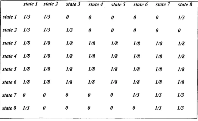
Table 1: Markov Transition Matrix Governing The Shocks 56 Table 2; Average, Maximum, and Maximum Kurtosis and Skewness,

1000 Simulations 59

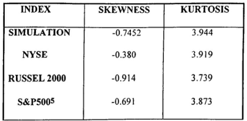
Table 3: Distributional Characteristics of Simulated Data

versus a Selection of U.S. Indices 60

Table 4; Distributional Characteristics for ret260 65

Table 5; GARCH (1,1) Equation Label in EVIEWS 69

Table 6: GARCH Conditional Mean in EVIEWS 69

Table?: GARCH Conditional Variance in EVIEWS 70

Table 8: ARCH-LM Test after GARCH is done, 15 Lags 75

Table 9: Forecasts Out-of-Sample Using GARCH and CHV 77

Table 10a: Forecast Evaluation of GARCH in 1,000 Simulations 81

LIST OF ILLUSTRATIONS

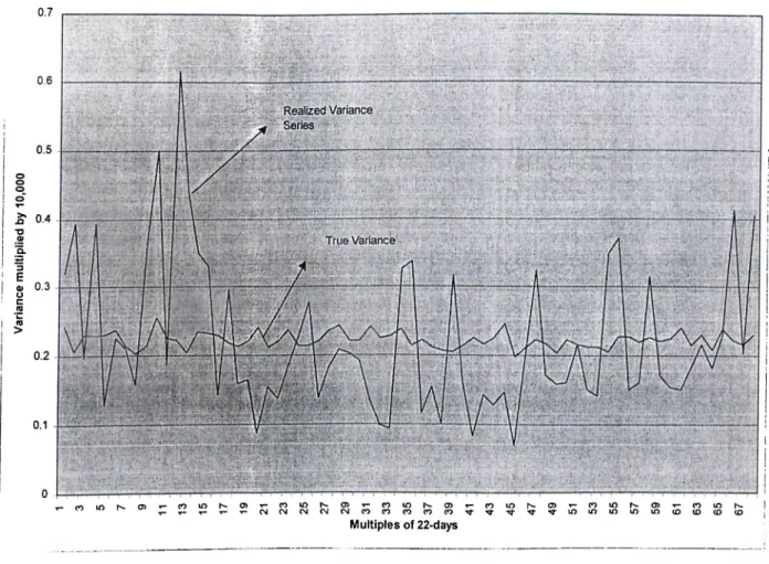
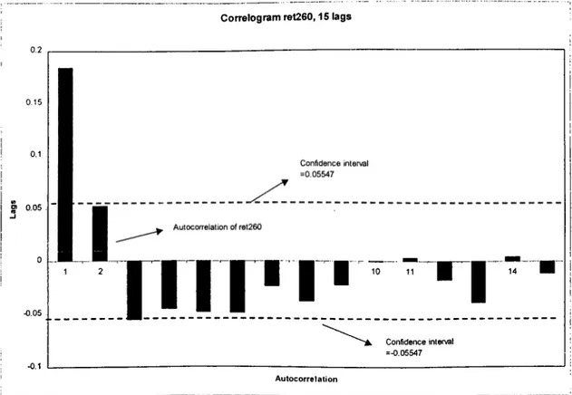
Figure 1: Realized Variance versus True Variance, 7-day steps Figure 2: Realized Variance versus True Variance, 22-day steps Figure 3: Correlogram of ret260 for 15 Lags

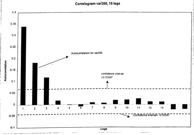
Figure 4: Correlogram of var260 for 15 Lags

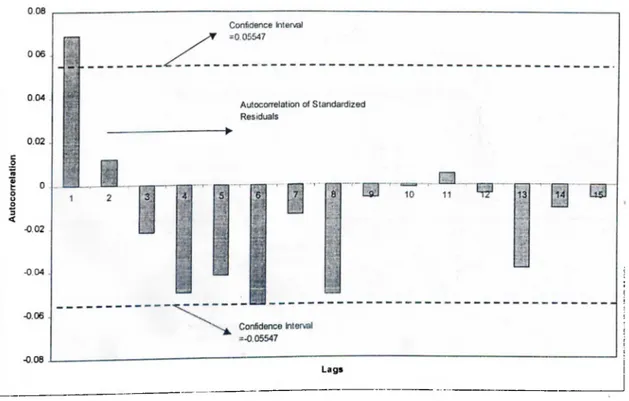
Figure 5; Correlogram of Standardized Residuals for 15 Lags

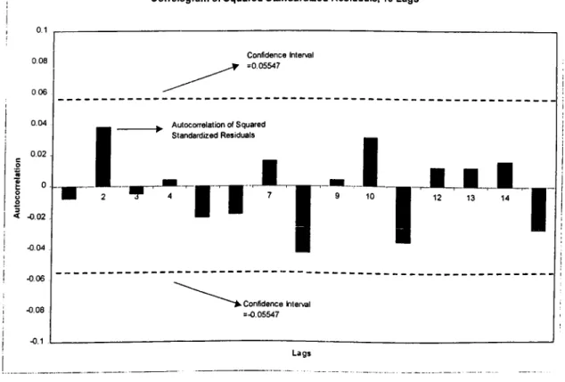
Figure 6: Correlogram of Squared Standardized Residuals for 15 Lags Figure 7: Out-of-Sample GARCH Forecasts Compared to True and Realized

Variance

Figure 8; GARCH Histogram of 7-day Ahead Forecasts Across All Simulations

Figure 9: CHV Histogram of 7-day Ahead Forecasts Across All Simulations

GARCH Histogram of 22-day Ahead Forecasts Across All Simulations

CHV Histogram of 22-day Ahead Forecasts Across All Simulations

Figure 10: Figure 11: 63 64 65 72 73 78 6 1 82 83 84 85

CHAPTER I INTRODUCTION

Financial market volatility is of central importance for a variety of market participants. The literature is in agreement that financial market volatility is predictable (see Bollerslev, Chou and Kroner (1992), Engle (1993), Engle and Ng(1993)) and time- varying (Schwert (1989). This has important implications for portfolio and asset management (Merton, 1980), and the pricing of primary and derivative assets (Baillie and Myers(1991) and Engle, Hong, Kane, and Noh (1992)). Expected volatility is a key ingredient of the pricing mechanism of such diverse financial assets as bond and equity futures, options, and common stocks (Ritzman, 1991). Estimates about volatility are routinely used by participants in the derivatives markets for hedging.

Performance of different volatility forecasting models have been proposed and tested in the literature. Among all the volatility forecasting models, the GARCH family has received the greatest attention in the literature. ARCH and GARCH modeling in finance has enjoyed a prominent and varied history in the literature since its inception by Engle (1982) and generalization by Bollerslev (1986). It is an indispensable, often

integral, part of many textbooks devoted to finance and econometrics. An overview of ARCH modeling in Tim, Chou, and Kroner (1992) has suggested and cited its use in the implementation and tests of competing asset pricing theories, market microstructure models, information transmission mechanisms, dynamic hedging strategies, and the pricing of derivative securities.

While most researchers agree on the predictability of stock market volatility (Engle and Ng, 1993; Engle, 1993), there is considerable variation of opinion on how this predictability should be modeled. The proliferation of research in the light of the evidence for predictability has led to a variety of approaches. The ARCH and GARCH models of Engle (1982) and Bollerslev (1986) respectively, and their many variants have been extensively used, and are among the broad class of parametric models that incorporate time dependency into the conditional variance underlying an asset return process'.

' As a prelude lo further discussion, some notation on the difference between conditional and unconditional moments, central to the intuition underlying ARCH and GARCH, is necessary. The following discussion on conditional and unconditional moments is based on Engle .(1993):

Let Vf be the return on an asset received in period t. Let E represent mathematical expectation. Then the mean o f the return can he called p, and

E y , = p ( I ! )

This is the unconditional mean, which is not a random variable. The conditional mean, nif, uses information from the previous periods, and can generally he forecast more accurately. It is given by:

m ,^ E [y tlF ,.i]^ E ,.,[y [] (L2)

This is in general a random variable o f the information set Fj,j. Note that, although Vf-F can be forecast, Vf-m cannot, using the information in Fi.j alone.

The unconditional and conditional variances can be defined in a similar way, as:

al = E [y rF p = Elyt-mt]^ + -Fp '

ht=Efllyr> ^tl

Models incorporating time dependence in the conditional variance, such as ARCH and GARCH, attempt to capture the well-known phenomenon of volatility clustering in financial data. Volatility clustering refers to the common occurrence in financial data whereby large shocks in magnitude to the return of a security tend to be followed by similarly high shocks of either sign.

The ARCH and GARCH type models of the conditional variance use the past values of the realized variance and shocks to forecast future variance. In so doing, the assumption of a constant variance over time is abandoned, and a structure governing the impact of past news is imposed (Engle and Ng, 1993). As such, the ARCH and GARCH type models explicitly incorporate recent news into the forecast of the future variance.

Alternative models of the volatility processes have also been proposed in the literature. Some of the most prominent are the historical variance models of Parkinson (1980), Garman and Klass (1980), Beckers (1983), and Abrahamson(1987), which will be discussed at length in Section II. These historical variance estimators use past historical price data to estimate a constant volatility parameter .

‘ Canina and Figlewski (1993), Figlcwski (1994), Lamoureux and Laslrapes (1993), and Pagan and Schwerl (1990) use the historical variance estimator in a comparative framework with ARCH and GARCH type models, and evaluate their respective performance in producing forecasts. A very readable and intuitive account o f the historical volatility estimator is provided by Ritzman (1991).

Historical volatility could be used as an ex-ante estimate of what market participants believed the volatility of an asset’s return would be over some future period in time (Gordon, 1991). However, historical volatility is unlikely to reflect investors’ changed expectations at a given point in time, such as in the event of a release of good or bad news (Ritzman (1991), Gordon (1991)). Consequently, a measure incorporating the markets expectation of aggregate future variance, the implied volatility, has been proposed as the market proxy for an asset’s average volatility over the remaining lifetime of the option written on the asset. The performance and limitations of the implied volatility model have been studied by Day and Lewis (1992), Canina and Figlewski (1993), and Lamoureux and Lastrapes (1993). Implied volatility is calculated from the Black-Scholes option valuation formula for a European Call Option:

C = C(5o,2r,£7,r,r) (1.5)

where C is the call option price, Sq is the stock price today, X is the option strike price, r is the risk-free rate, T is the time remaining to maturity, and a is the volatility. All variables but the latter are known, and thus cr can be solved for as follows:

„plied =cr{So,X,C,r,T) (

1

6

The market price of the (call) option thus reflects the market expectation of the assets average volatility over the remaining life of the option.

Although the Classical Historical Variance and Implied Volatility models fail to accomodate for the time-varying property of volatility, there is considerable evidence in the literature that volatility is in fact changing over time. For example, Schwert (1989) shows that the variations of volatility for monthly stock returns on the period 1857-1987 range from a low of 2% in the early 1960’s to a high of 20% in the early 1930’s. As noted before, taking this feature into account appeared to be vital for many areas of the financial literature: continuous-time models and option pricing, CAPM, investment theory, amongst others (Engle and Ng, 1993). Another line of attack into modeling the time variation in volatility that has been developed since the early 1980’s are continuous-time diffusion models with stochastic volatility (Hull and White(1980), Wiggins (1987), Chesney and Scott (1989))^.

As mentioned above, volatility forecasting is a vital ingredient in many applications. As a result, the performance of different volatility forecasts have been studied extensively in the literature. These studies have followed two directions. In- sample tests of volatility attempt to determine the model that fits the data well"*. However,

■ Hansson and Hordahl have investigated the performance o f stochastic volatility models using Swedish OEX index data (1996), and Nelson (1990) has shown that a GARCH process can be interpreted as a discrete-time approximation o f a diffusion model with stochastic volatility, thus connecting the two approaches.

^ Studies doing in-sample tests o f ARCH and GARCH point out the need to use a large number o f observations for the

model to fit the data well (Figlewski (1994), Pagan and Schwert (1991)). Figlewski (1994) reports the difficulties in implementing ARCH estimation to a group o f data sets. Lamoureux and Lastrapes (1993) observe that sophisticated ARCH type models with many parameters are needed to fit a data well, and the more parameters the model has. the worst its performance is in making forecasts “out-of sample*'. This study encounters little difficulty in fitting a

it is a well known fact that it is an easier task to develop a model that fits one's data well than it is to construct a model that makes good out-of-sample forecasts.

For out-of-sample tests, the definition of realized volatility is very important. The common practice is to compute realized volatility from the time-series return realization of the forecast horizon. Out-of-sample tests use forecasts obtained using the estimates of the model parameters, which are found in-sample'^, and subsequently compare these forecasts to realized volatility^. In the case of ARCH and GARCH, the in-sample is used to obtain maximum likelihood estimates of the ARCH parameters, then these estimates are used in an ARCH forecast equation to make forecasts for the out-of-sample period. To evaluate the forecasts, forecast error criteria such as Root Mean Squared Error (RMSE) and Mean Absolute Error (MAE) are used.

This approach ignores the possibility of different return realizations for each time, which is vital for drawing conclusions about perfonnance, as each different return realization in the forecast horizon would lead to a different conclusion about the performance of a model. In other words, a formal out-of-sample performance test of a given model would require that one should have the true distribution of returns for each

GARCH (1,1) model to a simulated group of 1,000 .sets o f data, o f 1,500 days each- chosen to correspond roughly to one business cycle.

^ Using a fixed window history o f price data.

^ In the case o f the classical historical volatility estimator, for example, a sample or history o f returns (what is referred to as the “in-sample") is taken, the standard deviation within this sample is computed, and this becomes the average standard deviation (the historical volalilil) м for the forecast period ahead (what is referred to as the “out-of-sample").

time from which one can calculate the true variance. The performance of forecasts could then be judged on how closely they predict this true \’ariance parameter in the forecast horizon. However in real life one can only observe one realization out of that distribution for each time, and this realized variance would be the best estimate of the true variance’

n

over the forecast horizon .

For longer forecast periods, realized volatility calculations used in the literature will be increasingly closer the true variance with large number of observations that resemble the true distributions. However for short forecast horizons this approach is extremely problematic. As a forecaster, one has to think about all the possible outcomes and probabilities assigned to those before making any forecasts.

In marked contrast to any existing work in the literature, this study proposes to find and use “true” daily volatility to explore the performance of GARCH. “True” variance on a given day is calculated via simulation of a computable general equilibrium model based on Akdeniz (1998) and Akdeniz and Dechert’s (1997) solution to Brock’s (1979,1982) multifirm stochastic growth model.

The wide range of findings and disagreements in the literature on GARCH performance^ can be better understood in the light of the failure to account for the “true”

^ Volatility and Variance are used interchangeably in this study. For reference, Variance is Volatility squared.

8

Assuming the realized return series is ergodic.

^ S ee Figlcwski (1994), Engle and Ng (1993), Lamoureux and Lastrapes (1993), Day and Lewis (1992), Pagan and Schwert (1990).

volatility as a performance basis when evaluating out-of-sample forecast performance of ARCH and GARCH. As observed by Bollerslev, Kroner, and Chou (1992), further developments concerning the identification and formulation of equilibrium models justifying empirical specifications for the observed heteroskedasticity remains a very important area for research. This study also aims to explore the performance of the GARCH specification for observed heteroskedasticity in contrast to naive estimators such as the classical historical volatility estimates.

In practice it is impossible to determine the true probability distributions of real economic time-series, but this study uses a stylized solution to Brock’s (1979, 1982) intertemporal asset pricing model in which the true distribution of returns is calculated, and thus known. This setting is particularly chosen because of its success in simulating real life business cycle data, and reconciling some of the contentions to which the Capital Asset Pricing Model (CAPM) has been subject. This suggests that it will be a powerful tool in resolving the forecast performance debate among various volatility forecasts including the GARCH family of models.

This study uses a particular form of Akdeniz (1998) and Akdeniz and Dechert’s (1997) solution to Brock’s (1979, 1982) model to test the performance of out-of-sample forecasts of Bollerslev’s (1986) GARCH(1,1) model. Brock’s model is simulated by using Akdeniz and Dechert’s (1997) solution 1,000 times to obtain 1,000 daily stock return data sets. Each simulated data set consists of the return realization for three firms

over a period of 1,500 days ( approximately one business cycle). The true distribution on any day can be obtained from these 1,000 simulation observations of the return process for that day.

The results demonstrate that the GARCH (1,1) model performs significantly better than historical volatility as measured by the MAE and RMSE criteria, when the true variance is used as benchmark. For forecasts 7-days ahead, GARCH (1,1) performs better than Classical Historical Volatility in 865 cases out of 1,000 simulations. It is found that Classical Historical Volatility has an MAE 4.832 times greater than GARCH (1,1), and an RMSE 4.003 times greater than GARCH across all simulations in this horizon. For a 22-day forecast period. Classical Historical Volatility is outperformed by GARCH(1,1) in 800 cases in 1,000 simulations, and has MAE 2.759 times as much, and RMSE 2.324 times as much as GARCH (1,1). Even more strikingly, it is found that if one were to use out-of-sample realized variance to evaluate forecast performance (as done in the literature) in each simulation, the RMSE and MAE for GARCH (1,1) would increase approximately three-fold, while decreasing significantly for Historical Volatility estimates. This demonstrates that the GARCH (1,1) model does a very good job of forecasting the true variance parameter in short-term horizons.

Using a single time series realization to study GARCH performance in the short­ term is analogous to “mixing apples and oranges”. An unfair realized volatility measure is certain to penalize GARCH forecast performance. The benefit of foreknowledge in the

form of the “true” volatility as a benchmark for forecast comparisons is used to demonstrate the potential of the GARCH family of conditional volatility models. Whilst highlighting an ingredient that has been missing in the relevant literature, this study offers a means of explaining why most studies have not been sufficiently able to provide a more accurate picture of how well GARCH type models perform.

This study proceeds as follows. Chapter II. provides an overview of the literature, including more detailed discussions of the conditional variance e.stimators used in the literature, and goes on to discuss the computational general equilibrium model of Brock (1979, 1982) and the solution to the model by Akdeniz and Dechert (1997) that is utilized here, as well as highlighting the role of computational economics in the literature. Chapter III. discusses the model and the numerical solution. Chapter IV. details the results, and Chapter V. presents conclusions.

CHAPTER II LITERA TURE REVIEW

II. 1 Introduction

Volatility is important to financial analysts for several important reasons. Estimates about volatility together with information about central tendency allow the analyst to assess the likelihood of experiencing a particular outcome. Volatility forecasts are particularly important for traders, portfolio managers and investors. Investors committed to avoiding risk, for example, may choose to reduce their exposure to assets for which high volatility is forecasted Traders may opt to buy options whose volatility they believe to be underpriced in the market, using their own subjective forecasts for volatility. The value of a derivative asset, such as options or swaps, depends very sensitively on the volatility of the underlying asset. Volatility forecasts for the underlying assets’ return are therefore routinely used by participants in the derivatives markets for hedging (see Baillie and Myers (1991), and Engle, Hong, Kane, and Noh (1992)). In a market where such forces operate, equilibrium asset prices would be expected to respond to forecasts of volatility (Engle, 1993).

Scholars and practitioners have long recognized that asset returns exhibit volatility clustering (Engle and Rothschild. 1992). It is only in the last decade and a half that statistical models have been developed that are able to accommodate and account for this dependence, starting most prominently with Engle’s (1982) ARCH and Bollerslev’s (1986) GARCH. A natural byproduct of such models is the ability to forecast both in the short and in the long run.

Given that volatility is predictable (Bollerslev (1992), Engle (1993), and Engle and Ng(1993)), it is clear that one must choose between alternative models of forecasting volatility to obtain an “optimal” forecast model. In particular, the choice must be made based on a clear set of criteria, such as long run or short run performance in a specific forecast horizon. Equally important, the criteria for performance must be carefully scrutinized for bias towards a particular model. What follows is a description of the most popular volatility forecasting models in the literature.

II.2 Forecasting Models in the Literature

n.2.1 GARCH(p,q):

The GARCH(p,q) was originally proposed by Bollerslev (1986) and is a generalization of Engle’s (1982) ARCH(p). A GARCH(p,q) model specifies that the conditional variance depends only on the past values of the dependent variable and this

relationship is summarized in the following equations; Yt X,n + 8, (2.1) sj4 ^ ..,~ N (0 ,a?) (2.2) /=1 (2.3) = ¿у + a{L)e] + /3{L)(7] (2.4)

In the GARCH(1,1) case, (2.4) reduces to:

= 6) + + у9,(Т^_ (2.5)

Here y, refers to the return on day t, x,n is the set of regressors, s, is the residual error of regression which is conditionally distributed as a normal random variable with mean zero and variance a]. Here a] is the conditional variance at time /, and is a

function of the intercept long run variance ---- ^ ---- , the squared residual from

\ - a - P

yesterday e]_^ (the ARCH term) and yesterday’s forecast variance<Т‘_| (the GARCH term).

today's variance by forming a weighted average of a long term average or constant variance, the forecast of yesterday (the volatility), and what was learned yesterday (or equivalently the shock). If asset returns were large in either way, the agent increases his estimate of the variance for the next day (Engle, 1996). This specification of the conditional variance equation takes the familiar phenomenon of volatility clustering in financial data into account, which is the property that large returns are more likely to be followed by large returns of either positive or negative sign, rather than small returns.

11.2.2 Historical Volatility

The most commonly used measure of volatility in financial analysis is standard deviation (Ritzman,1991). Standard deviation is computed by measuring the difference between the value of each observation on returns and the sample’s mean, squaring each difference, taking the average of the squares, and then taking the square root of this average. In mathematical terms, this is equivalent to

o-i,·/· = (2.6)

Where R| is the return on day i, R is the mean return in the sample 1, ..., T and the sum of squared differences is divided by T-I because the data under consideration is a sample.

and not the population.

The classical historical volatility estimates are computed in a similar fashion. The classical historical volatility estimate as defined by Parkinson (1980), Garman and Klass (1980), and other authors, as a forecast going N periods forward is simply the standard deviation of returns computed from the previous N periods. Equation (2.6) is thus the classical historical volatility estimate of the average volatility during days T+1, T+2, ..., 2T. An alternative classical volatility estimate, motivated by the lognormality of stock price returns property (Black and Scholes, 1973), can be obtained by computing the logarithms of one plus the returns, squaring the differences of these values from their average, and taking the squared root of the average of the squared differences. For short time frames (of the order of one or two months) it does not make much difference which version of the classical historical estimator is used (Ritzman, 1991).

Alternate estimators have been derived in an attempt to improve on the efficiency of the classical historical volatility (CHV) estim ator'w hich simply uses the variance of the market close-to-close return:

F ,"= (ln (Ä ,„/ln Ä ,)-R )^

f/" = _ J _ y w '

(2.7)

(2.8)

Where Cj denotes closing price at time /, and N is the number of periods. The classical historical volatility estimator is an estimate of the volatility using past history of data, and is used as a forecast of volatility over some future period.

All of these approaches are similar in that they assume the stock price follows a diffusion process with zero drift and constant volatility:

5 (2.9)

Based on this assumption, several authors develop measures which include more than the closing prices as estimators of the variance term adz.

Parkinson’s PK estimator (1980) of the variance of returns depends only on the high and low values, over each period. The statistic is the variance estimate over period i. To obtain an estimate of average variance over N periods, the high observed price Hi and the low observed price Lj , is cumulated to obtain V^, the average variance over N days: V.i’K = (ln(7^,)-ln(I,))^ 41n2 v ^ = — y (

2

10

The Garman and Klass (1980) estimator is an extension of the Klass estimator and develops a more accurate method of estimating the variance of the displacement (or diffusion constant cr) in a random walk. Garman and Klass (1980) assume that the logaritlun of stock prices follows a Brownian motion with zero drift, regardless of whether the market is open or closed. Their basic formula is given in equation (2.12), where Oj is the assets’ opening price and Cj is the closing price. The left-hand term is the squared difference between the open-to-high and open-to-close returns, while the right hand term is the squared open-to-close return:

In O J - In A

a .

2

12

oJ

The formula for situations when opening prices are not available (and the previous day’s close is used instead) is given by equation (2.14):

V/'>^= .5 [!n //,-ln I,f-.3 9 I n - ^C V

\ G ,_ |

J

weighted average of the PK estimator and the classical historical estimator.

When the market of interest does not trade 24 hours a day, the estimator to be used is given in equation (2.15). This version is simply a linear combination of the previous estimator (2.14) and a new estimator of the variance during the proportion of the day f when the market is closed:

f/G/C2=z ¡ 2 In O. C._;l -/ +.88 ya/c

w

II.2.3 Implied Volatility

There can be situations where an ex-ante estimate of what market participants believe the volatility of an assets’ return to be is needed. In such a case, a historical estimate, such as those described in section II.2.2, could be used. However, the historical estimate is unlikely to reflect investors’ changed expectations at a given point in time (e.g., in the event of the release of bad news). Consequently, it is necessary to focus some attention

on the concept of implied volatility, which is an attempt to estimate the aggregate expectations of future variance that the market has at a given point in time. If we believe that investors and speculators price options according to the Black and Scholes (1973) option pricing formula, then the price of a European Call Option is given by

c

= c(s„,x.a,r.T)

This also suggests that the implied standard deviation (ISD) of the option should be given by:

cr = cr(5o,X ,C ,r,r) (2.18)

Equation (2.18) can be solved by numerical search procedures, such as Ne\vton Raphson or the method of bisection (Ritzman (1991), Gordon (1991))".

II.2.4 Stochastic Volatility

The development here borrows heavily from the discussion of stochastic volatility to be found in Hansson and Hordahl (1996), Taylor (1994), Harveys, Ruiz and Shephard

Lalanc and Rendleman (1976), Palell and Wolfson (1981), Scmalanscc and Trippi (1978), MacBelh and Melville (1979), Manasler and Rendleman (1982j have examined the properties and investigated the difficulties with the use of ISDs in practice.

(1994), and Ruiz (1994).

From a theoretical point of view, it is useful to start with a continuous time specification for the price of an asset, while a discrete time approximation is generally used for estimation purposes. It is assumed, following Scott (1987) and Wiggins (1987), that the return of an asset dP/P follows a Geometric Brownian Motion while the logarithm of volatility follows an Omstein-Uhlenbeck process;

dP ! P = ccdt + adW,, (2.19a)

diner = -\n<j)dt + (fdW·^, (2.19b)

dW ,dW ^=pdt, (2.19c)

Wliere P(t) denotes the price of an asset at time i, a is the return drift, r is a parameter which governs the speed of adjustment of log-volatility to its long-term meani^, <p determines the variance of the log-volatility process, and {lfi(0>^2(0} is a two-dimensional Wiener process with correlation p.

In a discrete time approximation of the models above'^ the continuous return of an asset Vf, corrected for the unconditional meanju, is a martingale difference while the

logarithm of squared volatility In cr,- follows an AR(1) process;

r, = ln(P, ) - ln(/>„, ) - ^ = exp(/7, / 2 )s ,, f , ~ 7A[0.1]

(

.

)

/2,^1 = ^ + (f>h, +?!,, 7, ~ 7A^[0, cr: ] (2.21)

(2_.22₎

where Ô, and (j) are constants. The stochastic volatility for period t is at or exp(h,/2), and the realized value of the volatility process hj is in general not observable. The AR(1) process of the logarithm of variance, hj, is stationary if |^| < 1 and it follows a random walk if <j) =1.

IL3 Conditional Volatility Models in the Literature and Performance Studies

Performance of different volatility forecasts have been proposed and their performance tested in the literature. Among all the volatility forecasting models, the GARCH family has received the greatest attention in the literature. ARCH and GARCH modeling in finance has enjoyed a prominent and varied history in the literature since its inception by Engle (1982) and generalization by Bollerslev (1986). An entire volume of

the Journal of Econometrics was devoted to its use in research in 1992. It is an indispensable, often integral, part of many textbooks devoted to finance and econometrics. An overview of ARCH modeling in Tim, Chou, and Kroner (1992) has suggested and cited its use in the implementation and tests of competing asset pricing theories, market microstructure models, information transmission mechanisms, dynamic hedging strategies, and the pricing of derivative securities.

While it has been recognized for quite some time that the uncertainty of speculative prices, as measured by the variances and covariances, are changing over time [ e.g Mandelbrot (1963) and Fama (1965)], it is only somewhat recently that applied researchers in financial and monetary economics have started explicitly modeling time variation in second or higher-order moments. The Autoregressive Conditional Heteroskedasticity (ARCH) model of Engle (1982) and its various extensions have emerged as one of the most noteworthy tools for characterizing changing variances. More than several hundred research papers applying this modeling strategy have already appeared. Volatility is a central variable which permeates many financial instruments and has a central role in many areas of finance. As one simple example, volatility is vitally important in asset pricing models as well as in the determination of option prices. From an empirical viewpoint, it is therefore of no small importance to carefully model any temporal variation in the volatility process. It is important therefore that the performance of the ARCH model and its various extensions be tested in vitro in a simulated dynamic general equilibrium model that has already corroborated the theoretical results of the

САРМ and where the true distribution of the returns is known in its ex-ante form. It is a fact worth mentioning that there has been scant attention to this type of performance analysis of the GARCH family models in the relevant literature.

Implied and historical variance estimators have also received wide attention, and their empirical performance has been analyzed, both on a stand-alone basis, and in comparison with other conditional variance estimators. Figlewski (1994) examines the empirical performance of different historical variance estimators and of the GARCH(1,1) model for forecasting volatility in important financial markets over horizons up to five years. He finds that historical volatility computed over many past periods provides the most accurate forecasts for both long and short horizons, and that root mean squared forecast errors are substantially lower for long term than for short term volatility forecasts. He also finds that, with the exception of one out of five data sets used, the GARCH model tends to be less accurate and much harder to use than the simple historical volatility estimator for his application.

In another paper, Canina and Figlewski (1993) compare implied volatility estimators to historical volatility for S&P 100 index options, and find implied volatility to be a poor forecast of subsequent realized volatility. They also find that in aggregate and across sub-samples separated by maturity and strike price, implied volatility has virtually no correlation with future volatility, and does not incorporate the information contained in recent observed volatility.

Pagan and Schwert (1990) compare several statistical models for monthly stock return volatility using US data from 1834-1925. They use a two-step conditional variance estimator [Davidian and Carroll (1987)], a GARCH (2,1) model, an EGARCH(1,2) model [Nelson (1988)], Hamilton's (1989) two-state switching-regime model, a nonparametric kernel estimator based on the Nadaraya (1964) and Watson (1964) Kernel estimator, and a nonparametric flexible Fourier form estimator [Gallant (1981)]. They find that taking the 1835-1925 period as the sample, nonparametric procedures tended to give a better explanation of the squared returns than any of the parametric models. Of the parametric models. Nelson’s EGARCH comes closest to the explanatory power of the nonparametric models, because it reflects the asymmetric relationship between volatility and past returns. However, they also find that Nonparametric models fare worse in out-of- sample prediction experiments than the parametric models.

Lamoureux and Lastraspes (1993) examine the behavior of measured variances from the options market and the underlying stock market, under the joint hypothesis that markets are informationally efficient and that option prices are explained by a particular asset pricing model. They observe that under this joint hypothesis, forecasts from statistical models of the stock-return process such as GARCH should not have any predictive power above the market forecasts as embodied in option implied volatilities. Using in-sample and out-of-sample tests, they show that this hypothesis can be rejected, and find that implied volatility helps predict future volatility. Using the analytical framework of the Hull and White (1987) model, they characterize stochastic volatility in

their data by using the GARCH model. Their out-of-sample tests show that GARCH does not outperform the classical historical volatility estimator significantly. GARCH, Historical Volatility, and Implied Volatility are each used to forecast the mean of the daily variance over the remaining life of the option. For each day in the forecast horizon, each forecast is compared to the actual mean of the daily realized variance. In a bid to compare their results with other studies, they refer to Akgiray (1989). Using the root mean squared error (RMSE) criterion for stock index data, Akgiray (1989) finds that, at a forecast horizon of 20 days, GARCH variance forecasts are convincingly superior to historical volatility. Lamoureux and Lastrapes (1993) replicate Akgiray’s (1989) analysis with a 100 day forecast horizon and find that the relative rankings of historical volatility and GARCH are overturned. They also find that implied variance tends to underpredict realized variance, as evinced by a significantly positive mean error (ME) in their study. They also observe that, as GARCH weights the most recent data more heavily, GARCH overstates the frequency of large magnitude shocks, which leads to good in-sample fit and excellent short-term forecasts, but poor long term forecasts (see also Akgiray(1989) and Nelson (1992)).

Day and Lewis (1992) compare the information content of the implied volatilities from call options on the S&P 100 index to GARCH and Nelson’s EGARCH models of conditional volatility. By using the implied volatility as an exogenous regressor in the ARCH and EGARCH models, they examine the with-in sample incremental information content of implied volatilities and the forecast from GARCH and EGARCH models.

Their out-of-sample forecast comparisons suggest that short-run market volatility is difficult to predict, and they conclude that they are unable to make strong statements concerning the relative information content of GARCH forecasts and implied volatilities.

Jorion (1995) examines the information content and forecast power of implied standard deviations (ISDs) using Chicago Mercantile Exchange options on foreign currency futures. Defining the realized volatility in the conventional sense , he regresses

realized volatility on forecast volatility'"’ and a time series volatility specification

modeled as GARCH (1,1), in the following way:

(y , j — a + + Eij (2.23)

This regression is used to test whether GARCH (1,1) forecasts have predictive power beyond that contained in cr™. In other words, Jorion tests whether the coefficient of the GARCH forecast, b j, is significantly different from zero. GARCH forecasts are obtained by successively solving for the expected variance for each remaining day of the options life, then averaging over all days. He finds that MA(20) and GARCH (1,1) forecasts have lower explanatory power than ISDs'^. He concludes that his results indicate option- implied forecasts of future volatility outperform statistical time-series models such as

'3 The realized volatility o f returns from day t to day T is thus the standard deviation o f returns in days t, t + l , .... f (Ritzman, 1991).

• ‘t Where the forecast volatility is taken to be the ISD forecast o f volatility o f returns over the remaining contract life. '5 lorion finds that the slope coefficient b2 o f the GARCH (1,1) forecast becomes small and insignificant, implying low forecast power compared to ISD.

GARCH in the foreign exchange market'*’, although the volatility forecasts of ISDs are biased- suggesting ISDs to be too volatile. It is worth extra emphasis that .lorion conforms to the existing practice in the literature of utilizing the realized variance, in this case in the foreign exchange market for three currencies, for forecast comparison regressions.

West and Cho (1995) compare the out-of-sample forecast performance of univariate homoskedastic, GARCH'^, autoregressive, and nonparanietric models for conditional variances, using five bilateral (Canada, France, Germany, .lapan, and the United Kingdom) weekly exchange rates for the dollar, for the period 1973-1989. They compare the out-of-sample realization of the square of the weekly change in an exchange rate with the value predicted by a given model of the conditional variance for horizons of one, twelve, and twenty four weeks. The performance measure that they use is the mean squared prediction error (MSPE), using rolling and expanding samples for the out-of- sample forecasts. For one-period horizons, they find some evidence favoring GARCH models. For twelve and twenty-four-week ahead forecasts of the squared weekly change, they find little basis for preferring one model over another. At the one-week-ahead forecast horizon, they report that GARCH (1,1) produces slightly better forecasts in the MSPE sense, but they conclude that statistical tests cannot reject the null hypothesis that the MSPE from GARCH (1,1) is equal to the MSPE from other models at all horizons considered. They observe that, based on this inability to reject the null, there are no viable

This is in sharp contrast to Canina and Figlcwski (1993), who find that ISDs have poor performance in the U.S. stock market.

More specifically, GARCH (1,1) and ICiARCH (1.1) models are used. These are selected because in-sample diagnostics are found to be better than other GARCH models.

reasons for preferring one model over another at all the horizons considered. It thus appears that GARCH performance leaves something to be desired, and although the GARCH models perform well, endorsement of these models is moderate. Although the in-sample evidence in their study clearly suggests that a homoskedastic model should be strongly dominated by the other models, they find this not to be the case. This is a surprising result, as the authors themselves acknowledge. There is one comment in their paper that is definitely worth reproducing in the context of this study: “...it might be largely a matter of chance which model produces the smallest RMSPE'*”. This element of chance is best explained and understood in terms of the use of realized out-of-sample variance, and this observation of West and Cho is one of the few veiled references in the literature to the arbitrariness of evaluating performance on the basis of a sample realization in the forecast horizon (which introduces the “chance” factor in performance referred to in the quotation), and the lack of formal tests of performance.

Amin and Ng (1990) study the asymmetric/leverage effect in volatility in option pricing. The asymmetric/leverage effect is a property of stock returns which has been the subject of much recent study (Black (1976), Christie (1982), French, Schwert and Stambaugh (1987), Nelson (1990), Schwert (1990)) and refers to the phenomenon whereby whereby stock return volatility is higher following bad news than good news. They find that a comparison of the mean absolute option pricing error under the GARCH, EGARCH, and Glosten, .lagganathan, and Runkle (GJR, 1992) models relative to the

mean absolute option pricing error under a constant volatility model favors EGARCH and GJR models.

Hansson and Hordahl (1996) estimate the conditional variance of daily Swedish OMX-index returns for the period January 1984-February 1996 with stochastic volatility (SV) and GARCH models. They find that the best in-sample fit is provided by the asymmetric unrestricted SV model with a seasonal effect. An evaluation of the forecasting power of the model is shown to provide better out-of-sample forecasts than GARCH models. They conclude in their study that the SV model specification is the preferred model for forecasting purposes.

Long memory processes and modeling aspects is another area that is exciting considerable interest in the GARCH literature. Bollerslev and Mikkelsen (1996) introduce a new class of fractionally integrated GARCH and EGARCH models to characterize U.S. financial market volatility. Recent empirical evidence indicates that apparent long-run dependence in U.S. stock market volatility is best accounted for by a mean-reverting fractionally integrated process'^. After in-sample estimation of various^** models on the Standard and Poors index, the authors simulate the price paths of options of different maturities with three alternative pricing schemes, and make option price forecasts for the three different EGARCH and an AR(3) data-generating mechanisms. At

•9 In such a process, a shock to the optimal forecast (grounded in the model) o f the future conditional variance decays a slow hyperbolic rale.

70-days to maturity, the lEGARCH model results in the highest forecast prices, whereas the homoskedastic AR model unifonnly produces the lowest valuations. The prices for EGARCH and FIEGARCH are very close. As the maturity increases to 270 days, the prices generated by FIGARCH are between EGARCH and lEGARCH valuations. The AR(3) model consistently underprices long and short horizon options, and the FIGARCH model appears to be the best candidate for characterizing the long-run dependencies in the volatility process of the underlying asset.

II.4 The Computable Dynamic General Equilibrium Model

11.4.1 Introduction

This study uses the method employed by Akdeniz and Dechert (1997) to solve the multifirm stochastic growth model of Brock (1979). Brock’s model reflects the utility maximizing behavior of the consumer and the profit maximizing behavior of the producers. The computational solution to Brock’s model produces results that resemble the “real” economy very closely and hence it is a very powerful tool with a rich variety of possible future applications. Many empirical anomalies, in particular the predictions of the Capital Asset Pricing Models (CAPM) and the contentions surrounding whether its predictions hold or not, have been resolved in the computational economy framework via

the approach by Akdeniz (1998) and Akdeniz and Dechert (1997)^'. The power of this computational framework as a general tool is thus particularly chosen to study the performance of the GARCH model, and the economy that it simulates can be made to mirror stock market data very closely, having all the properties that empirical data possess such as excess kurtosis, conditional moment dependence on time, volatility clustering, etc. This is just one of the many possible applications that Brock’s model, via the numerical solution of Akdeniz and Dechert (1997), can be put in to use.

The next section will discuss the mulifirm stochastic growth model and asset pricing model of Brock (1979, 1982), and prepare the ground for discussions on the particular numerical solution method adopted for this study, which will be presented in Section III.

11.4.2 The Growth Model

The model used as the basis in this study is the optimal growth model with uncertainty. The long-run behavior of the deterministic one-sector optimal growth model has been studied by Cass (1965) and Koopmans (1965), who showed the existence of a steady state solution. The extension of this model to include uncertainty can be found in Brock and Mirman (1973) and Brock (1979, 1982). This study utilizes the case of

discrete Markov process driven technology shocks. There is an infinitely lived representative consumer who has preferences over sequences of consumption gi\'en by the following expression:

E o \ ^ P 'u { c , ) \ , 0< y9< l, (2.24)

./=0

where c, denotes consumption of the single good, and denotes expectation conditional on information at date zero. There are N production processes in this economy that can be used to produce one type of good that can be consumed or added to the capital stock. The following discusses the growth model in some depth, and borrows heavily from Akdeniz and Dechert (1997). The key elements of the model are recapitulated as follows^^. max c, ,x„ and (2.25) N X. = E x i. i = l (2.26) i = l (2.27) C,+X. =y. (2.28) c,x, >0 (2.29) y^ historically given

Where: E

P

discount factor (constant) on future utility utility function of consumption^^

consumption at date t capital stock at date t output at date t

production function of process i plus undepreciated capital capital allocated to process i at date t

depreciation rate for capital installed in process i random shock

Observe here that fi(Xi,,^,) = gj(Xi,,^,) + (l-6i)X j,, where g^Cx^,,^,) is the production function of process i, and (1 - is remaining (undepreciated) capital after production in process i.

The optimal policy functions for consumption and investment for the representative consumer are obtained via maximization of the expected value of the discounted sum of utilities over all possible consumption paths and capital allocations^'*. The following explanation is offered by Brock to elucidate the working of the model:

23 The utility function is characterized b> u : is strictly concave, strictly increasing, and continuously dilTercnliabie with u(())=(), U ‘(0)=oo anci

“There are N different processes. At date / it is decided how much to consume and how much to hold in the form of capital. It is assumed that capital goods can be costlessly transformed into consumption goods on a one-for-one basis. After it is decided how much to hold in the form of capital , then it is decided how to allocate capital across the N processes. After the allocation is decided nature reveals the value of rj, and g,(x., ,r,) units of new production are available from process i at the end of period t. But bjXjt units of capital have evaporated at the end of period t. Thus, the net new produce is g.(x., ,r,)- 5jXi, from process i. The total produce available to be divided into consumption and capital stock at date t+\ is given by i][g,(x«> r,)-S*xJ + x, = l][g ,(x „ ,r,) + ( l - 5 J x J i = l ¡=1 N i = l where f(x,,T ,) = gi(x,,r,) + (l-5 ,)x „

denotes the total amount of produce emerging from process i at the end of period t. The produce y,..] is divided into consumption and capital stock at

the beginning of date /+1, and so on it goes”.

This study introduces a notational difference. Observe that Brock uses “r,” for his shock parameter, whereas in this study the shock parameter is denoted ”. The main assumptions for the model in this study are^^:

(Al) the functions u and fj are concave, increasing, twice continuously differentiable, and satisfy the Inada conditions;

(A2) the stochastic process is a discrete Markov process with eight states of uncertainty for each production process;

(A3) the maximization problem has a unique optimal solution.

Then the first order conditions for the intertemporal maximization can be written as:

u'(c,.,) = PE,.,[u’(c,)f'(x ,4 ,)] (2.30)

!H"P'E,-,[u'(c,)x„] = 0 (2.31)

It is worth mentioning that Equation (2.30) will be the one used in the following sections to obtain a numerical solution to the growth model. Obser\ ing that the problem given by equations (2.25) to (2.29) is time stationary, the optimal levels of c,, x,, are functions of the output level y,, and can be written as;

c, =g(y,) X, = h(y.) X, = h ,(y ,) (2.32)

Now the aim is to solve the growth model for the optimal investment functions, hj, and then to analyze the underlying implications of the asset pricing model. As a further simplification, note that the first two functions in equation (2.32) can be expressed in terms of these investment functions:

h(y) = i]h ,(y )

i = l

c(y) = y -h (y )

(2.33) (2,34)

II.4.3 The Asset Pricing Model

Brock’s (1982) asset pricing model has many characteristics in common with the Lucas (1978) model. The primary feature seperating the two models is that Brock’s model includes production. The inclusion of shocks to the production processes in the model directly links the uncertainty in asset prices to economic fluctuations in output

levels and profits.

The asset pricing model closely resembles the growth model discussed in Section 11.4.2. There is an infinitely lived representative consumer whose preferences are given by equation (2.24 & 2.25). The production side consists of N different firms. Firms maximize profits by renting capital from the consumer side:

(2.34) Each firm takes the decision of hiring capital after the shock is revealed. The interest rate in industry i at time t is determined within the model. Following the convention in the literature, asset shares are normalized so that there is one (perfectly divisible) equity share for each firm in the economy. Thus, ownership of a proportion of the share of firm i at time t grants the consumer the right to that proportion of firm i’s profits at time t+1. Following Lucas (1978), it is assumed that the optimal levels of output, consumption, asset prices, and capital form a rational expectations equilibrium.

The representative consumer then solves the following problem:

max E ¿ P 'u ( c ,)

IN

subject to: c, +x, +P, -Z, <ti, -Z,., +P, -Z,_, +2r.^,..,x.^,_

(2.35)

C,, Z,, X, >0 (2.37) (2.38) (2.39) Where:

R, price of one share of firm ; at date t.

Z^, number of shares of firm / owned by the consumer at date 1. t:., profits of firm / at date h

Again, for details of the model, refer to Brock (1982). First order conditions derived from the maximization problem are:

and

Pi.u'(c,) = pE,[u'(c,,,)(Tr.^ +Pi„,)]

u'(c,) = pE,[u'(c,^,)f'(x.,„,^,„)]

(2.40)

(2.41)

The first order conditions yield the prices for the assets. However, the transversality conditions

WmP' E( u\c,)Y^P„Z„ = 0 (2.42)

are required to fully characterize the optimum^^. This condition, as noted by Judd (1992), suggests that we are looking for a bounded solution^’ to the growth model. Brock (1979) has shown that there is a duality between the growth model (2.25-2.29) and the asset pricing model (2.35-2.39). Thus the solution to the growth model also solves the asset pricing model. Once the solution to the former is found, equation (2.40) can be used to solve for the asset prices, and asset returns. To be more specific, once the optimal policy functions, hj(y), for the growth problem are obtained asset prices and asset returns can easily be calculated for given values of shocks.

II.5 The Model and Computational Economics in the Literature

In general no closed form solutions for stochastic growth models exists, except for the specific cases of logarithmic utility and Cobb-Douglas production functions with 100 percent discounting, and carefully paired CES production and utility functions" . The recent advances in computer hardware and computational methods have enabled economists to study these models. As a result, more and more economists have been using computational methods to solve dynamic economic models over the past two decades.

26 Brock (1982) shows that the transversalily condition holds in this model. 22 The optimal solution remains in a bounded interval: 0<a<V(<b<oo for all t.

Sims (1990) solves the stochastic growth model by backward-solving, a class of methods that generates simulated values for exogenous forcing processes in a stochastic equilibrium model from a specified assumed distribution for Euler-equation disturbances, with a particular nonlinear form for the decision rule. The backward-solved simulations, whose solution paths were shown to be stationary (Sims, 1989), are applied to a one- sector neoclassical growh model with decision rule generated from a linear-quadratic approximation. Baxter, Crucini, and Rouwenworst (1990) solve the stochastic growth model by a discrete-state-space Euler equation approach. They focus on the Euler equations that characterize equilibrium behavior, and then compute approximations to equilibrium decision rules. Their approach is “exact” in the sense that their approximate decision rules converge to the true decision rule as the grid over which the decision rules are computed becomes arbitrariliy fine. Their approach to simulute the economy’s respononse to shocks relies on Tauschen’s (1986) method to generate a sequence for the technology shocks, and using their approximate policy function together with the resource constraint to determine associated equilibrium values of output, consumption, and investment. Benhabib and Rustichini (1994) provide exact solutions for a class of stochastic programming problems in growth theory, specifically those involving pairs of constant relative risk aversion utility functions and CES technologies. They incorporate depreciation schemes into their model, and generalize the solutions for the well-known case of logarithmic utility coupled with Cobb-Douglas production functions .

A more thorough description and comparison o f .some o f the various methods can be found in Taylor and IJhIig (1990), and Danlhinc and Donaldson (1995).

A series of important observations made by Judd (1995) emphasize the relevance of computational methods for science in general and economics in particular. Judd (1995). in surveying the interaction between economic theory and computational economics, discusses the methodological issues raised by the idea of “computational theory”, and the problems associated with its dissemination and exposition. It is important to evidence what computational methods is not. At the most obvious, computational economics is not a theoretical proof of a proposition, in the sense that a proof is a logical-deductive process in which a proposition is formulated, and auxiliary assumptions are added (such as linear demand, constant costs, etc.) to the basic ones in order to make a proof of the proposition possible. Computational methods have complementary strengths and weaknesses relative to theoretical methods. They can approximately solve an arbitrary example of the basic theory, and determine the nature of any individual point in the solution space being explored. The advantage is that computational methods do not need as many, if any, auxiliary assumptions to compute the equilibrium. The supposed weakness is that they can do this only one example, one point, at a time, and in the end can examine only a finite number of points. Some argue that deductive theory has a superiority in that its results are error free. This has to be balanced with the self-evident limitations of an approach that is exclusively limited to a small subset of examples that obey the conditions imposed to make the analysis tractable. Although computational methods often involve error, their superior range offers an advantage.