■ F m O J E € T 2 Ü 2 € g «v-r'î»’ï.;T*?rrw7^-5:®7^; >r^,r¡ G·^' JLKÍJ » ÄJ2. ЛІЧ i-i· s--’¿^ Â4İİ.’-:câ^4 ;^' ,;„.-д, í5f?t· ^Τ'·^"·> ΐ^ '‘W i l l* 4»λ!< ji,«www¿.’ikJ*.«»·*.^* í w / «*;'’■>* iá. í *» *w* t'vr -p ή ? w r n ;^4X í 1^122
j U . · « . ¿ Г J b y - W i l , .-** ^ M» ■ w ~ . .vu, o*».*»,.»», . . « ^ . O - í V V ,u . İU.J
•PA'S ^^%TW: TrF ■“'^.‘рт:·'^^. гч^ *^ѵ: /Т· ^'"·. '■ ' ·Γ"4'’■ν’' ’ ■T'''V 'Ί' i* ·.**''' IlH A ^í -u y s a l 4^?4·'·· '·»■ ^U.'·"*^·«··.» ’■.·: » тЧ^'-;»г' 'щ '
'//â?
2 .0 0 0PR O JE C T IO N S
A THESIS
SUBMITTED TO THE DEPARTMENT OF COMPUTER ENGINEERING
AND THE INSTITUTE OF ENGINEERING AND SCIENCE OF BILKENT UNIVERSITY
IN PARTIAL FULFILLMENT OF THE REQUIREMENTS FOR THE DEGREE OF
MASTER OF SCIENCE
by
İlhan Uysal
January, 2000
Assoc. Prof. D r/flalil Altay Güvenir (Advisor)
I certify that I have read this thesis and that in my opinion it is fully adequate, in scope and in quality, as a thesis for the degree of Master of Science.
Assoc. Prof. Dr. Kemal Oflazer
I certify that I have read this thesis and that in my opinion it is fully adequate, in scope and in quality, as a thesis for the degree of Master of Science.
Approved for the Institute of Engineering and Science:
Prof. Dr. M ehm di^aray
INSTANCE-BASED REGRESSION BY PARTITIONING
FEATURE PROJECTIONS
Ilhan Uysal
M.S. in Computer Engineering
Supervisor: Assoc. Prof. Halil Altay Güvenir January, 2000
A new instance-based learning method is presented for regression problems with high-dimensional data. As an instance-based approach, the conventional K-Nearest Neighbor (KNN) method has been applied to both classification and regression problems. Although KNN performs well for classification tasks, it does not perform similarly for regression problems. We have developed a new instance-based method, called Regression by Partitioning Feature Projections (RPFP), to fill the gap in the literature for a lazy method that achieves a higher accuracy for regression problems. We also present some additional properties and even better performance when compared to famous eager approaches of machine learning and statistics literature such as MARS, rule-based regression, and regression tree induction systems. The most important property of RPFP is that it performs much better than all other eager or lazy approaches on many domains that have missing values. If we consider databases today, where there are generally large number of attributes, such sparse domains are very frequent. RPFP handles such missing values in a very natural way, since it does not require all the attribute values to be present in the data set.
Keywords: Machine learning, instance-based learning, regression.
ÖZNİTELİK İZDÜŞÜMLERİNİN PARÇALANMASI İLE
ÖRNEKLERE DAYALI REGRESYON
Ilhan Uysal
Bilgisayar Mühendisliği, Yüksek Lisans Tez Yöneticisi: Doç. Dr. Halil Altay Güvenir
Ocak, 2000
Yüksek öznitelik sayılarına sahip verilerin regresyon çözümleri için örneklere dayalı yeni bir öğrenme metodu sunulmuştur. Örneklere dayalı bir yaklaşım olarak geleneksel K-Yakm Komşu (KNN) yöntemi hem sınıflandırma hem de regresyon problemleri için uygulanmıştır. KNN sınıflandırma işlemleri için iyi bir performans sergilerken, regresyon için benzer bir performansa sahip değildir. Biz literatürdeki bu boşluğu doldurmak üzere, tembel öğrenme yaparak yüksek başarı sağlayan örneklere dayalı yeni bir regresyon yöntemi olan, Öznitelik İzdüşümlerinin Parçalanması ile Regresyon (RPFP) isimli yöntemi geliştirdik. RPFP makina öğrenmasi ve istatistik literatüründe yer alan MARS, kurallara dayalı regresyon ve regresyon ağacı öğrenen sistemler gibi önemli çalışkan al goritmalarda dahi bulunmayan bazı özelliklere ve hatta daha iyi performansa sahiptir. R P F P ’nin bu özelliklerinden en önemli olanı verilerde eksik değerler olduğu durumlarda pek çok uygulama için diğer tüm çalışkan veya tembel yöntemlerden daha çok başarı sağlamasıdır. Günümüzde, çok sayıda alanları bulunan veri tabanlarını dikkate aldığımız zaman, böyle ortamlara sıklıkla rast lanır. RPFP veri seti içindeki tüm öznitelik değerlerinin doldurulmuş olmasını gerektirmediği için eksik olan değerleri doğal bir şekilde çözümler.
A n a h ta r Sözcükler: Makina öğrenmesi, örneklere dayalı öğrenme, regresyon.
I would like to express my gratitude to Dr. H. Altay Güvenir, from whom I have learned a lot, due to his supervision, suggestions, and support during this research.
I am also indebted to Dr. Kemal Oflazer and Dr. Ilyas Çiçekli for showing keen interest to the subject m atter and accepting to read and review this thesis.
I would like to thank to Yeşim and Gözde, for their great patience and support that was very important, Halise for her support and data sets she provided, Nurhan for her morale support and Munise for many things.
I would also like to thank to Bilkent University Computer Engineering Department and Turkish Navy, since they enabled and supported this research.
This thesis was supported, in part, by TUBITAK (Scientific and Technical Research Council of Turkey) under Grant 198E015.
1 Introduction 1
1.1 Parametric versus Non-Parametric R e g ressio n ... 3
1.2 Eager versus Lazy L e a r n in g ... 4
1.3 Regression by Partitioning Feature P rojections... 5
1.4 N o ta tio n ... 6
1.5 Organization 6 2 O verview of Regression Techniques 7 2.1 Instance-Based R egression... 7
2.2 Locally Weighted Regression... 9
2.2.1 Nonlinear Local Models 10 2.2.2 Linear Local Models 10 2.2.3 Im plem entation... 11
2.3 Regression by Rule I n d u c tio n ... 12
2.4 Projection Pursuit R eg ressio n ... 16
2.4.1 Projection Pursuit Regression A lg o rith m ... 17
2.5 Regression by Tree Induction 20
2.5.1 C A R T ... 21
2.5.2 R E T IS ... 26
2.5.3 M 5 ... 28
2.6 Multivariate Adaptive Regression S p lin es... 29
2.6.1 Piecewise Parametric Fitting and S p lin es... 30
2.6.2 MARS A lgorithm ... 30
2.7 Discussion ... 33
3 R egression by Partitioning Feature P rojections 36 3.1 RPF'P A lg o rith m ... 39
3.1.1 T ra in in g ... 39
3.1.2 Approximation using Feature Projections... 40
3.1.3 Local W e ig h t... 43 3.1.4 Partitioning A lg o rith m ... 45 3.1.5 P re d ic tio n ... 48 3.2 RPFP-N A lgorithm ... 49 3.3 Properties of R P F P ... 51 3.3.1 Curse of Dimensionality 51 3.3.2 Bias-variance T rade-off... 54
3.3.3 Model Complexity and Occam’s R a z o r ... 55
3.3.5 Local L e a r n in g ... 57
3.3.6 Irrelevant Features and D im ensionality... 58
3.3.7 Context-sensitive L earn in g ... 59
3.3.8 Missing Feature V alu es... 60
3.3.9 In te ra c tio n s... 61
3.3.10 Feature Projection Based L e a r n in g ... 61
3.3.11 Different Feature Types 62 3.3.12 N oise... 62
3.3.13 N orm alization... 63
3.4 Limitations of R P F P ... 63
3.4.1 Redundant Features 63 3.4.2 In terp reta tio n ... 64
3.4.3 Rectangular R e g io n s ... 64
3.5 Complexity A n a ly s is ... 65
3.6 Comparisons of Regression M ethods... 65
4 Em pirical Evaluations 67 4.1 Performance M easure... 68
4.2 Algorithms Used in C o m p a riso n s... 68
4.2.1 R P F P ... 69
4.2.2 K N N ... 69
4.2.4 DART 69
4.2..5 MARS 70
4.3 Real Data Sets 70
4.4 Accuracy 70 4..5 Robustness to Irrelevant F e a tu r e s ... 72 4.6 Robustness to Missing V a lu e s ... 75 4.7 Robustness to Noise 75 4.8 Interactions, 79 4.9 Computation Times . 82
2.1 The Proximity Algorithm 8 2.2 2d-tree data structure. The black dot is the query point, and
the shaded dot is the nearest neighbor. Outside the black box does not need to be searched to find the nearest neighbor. 12
2.. 3 Swap-1 A lgorithm ... 13
2.4 A solution induced from a hart-disease d a t a ... 14
2.. 5 Composing Pseudo-Classes ( P - C la s s ) ... 15
2.6 Overview of Method for Learning Regression Rules 16 2.7 Projection Pursuit Regression A lg o rith m ... 18
2.8 Running Medians of T h r e e ... 19
2.9 Variable Bandwidth Smoothing A lg o rith m ... 20
2.10 Example of Regression T r e e ... 22
2.11 An example of the tree construction of process. Four regions are determined by predictors Xi and X2... 23
2.12 Recursive Partitioning A lg o rith m ... 24
2.13 A binary tree representing a recursive partitioning regression model with the associated basis functions... 25
2.15 MARS A lg o rith m ... 33 2.16 An example for the regions of MARS a lg o r ith m ... 33
3.1 An example training set projected to two features:/i and /2. . . 40 3.2 Approximations for Feature Projections 42 3.3 Example data set and its partitioning. 46 3.4 Partitioning A lg o rith m ..., . ... 47 3.5 Example training set after partitioning. 49 3.6 Approximations for Feature Projections 49 3.7 Prediction A lgorithm ... 50 3.8 Weighted Median A lgorithm ... 51
4.1 Relative errors of algorithms with increasing irrelevant features. 74 4.2 Relative eiTors of algorithms with increasing missing values. 77 4.3 Relative errors of algorithms with increasing target noise... 80 4.4 Artificial data set. x l and x2 are input features... 81
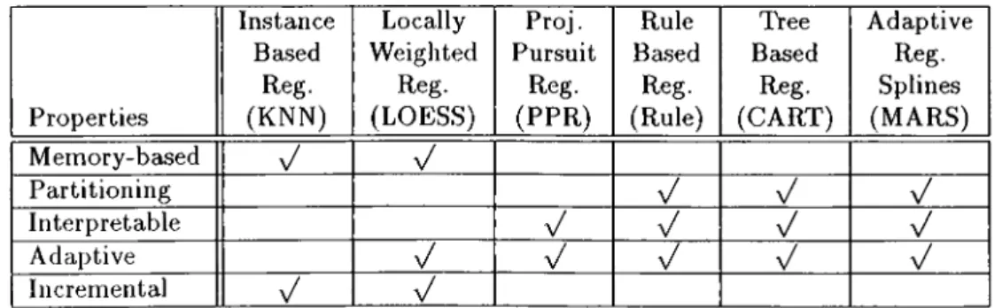
2.1 Example of swapping rule components... 14 2.2 Properties of Regression Algorithms (the names of programs de
veloped with those methods are shown in parentheses)... 35
3.1 Properties of Regression Algorithms. The (^Z) is used for cases if the corresponding algorithm handles a problem or it is advan tageous in a property when compared to others... 66
4.1 Characteristics of the data sets used in the ernpiriccil evaluations. C: Continuous, N: Nominal... 71 4.2 Relative Errors of Algorithms. Best results are typed with bold
font... 73 4.3 Relative errors of algorithms, where 30 irrelevant features are
added to real data sets. If the result is not available due to singular variance/covariance matrix, it is shown with (*). Best results are typed with bold font... 76 4.4 Relative errors of algorithms, where 20% of values of real data
sets are removed. If the result is not available due to singular variance/covariance matrix, it is shown with (*). Best results are typed with bold font... 78 4.5 Comparison of RPFP with its additive version RPFP-A. Best
results are typed with bold font... 81 xiii
B /5 CART CFP COFI D DART DNF / 9 H I i IBL K k KMEANS KNN KNNFP KNNR KDD L LOFiSS LOF log LW LWf LWR MAD MARS M5 n Basis Function Parameter set
Classification and Regression Trees Classification by Feature Partitioning
Classification by Overlapping Feature Intervals Training Set
Regression tree induction algorithm Disjunctive Normal Form
Approximated Function Approximated Function Step Function Fitting Function Instance Instance-based Learning Kernel Function
Number of Neighbor Instances Partitioning clustering algorithm K Nearest Neighbor
K Nearest Neighbor on Feature Projections K Nearest Neighbor Regression
Knowledge Discovery in Databases Loss Function
Locally weighted regression program Lock of Fit Function
Logarithm in base 2 Local Weight
Local weight of feature / Locally Weighted Regression Mean Absolute Distance
Multivariate Adaptive Regression Splines Regression tree induction algorithm Number of training instances
PPR q Xq R Rk R E RETIS RFP RPFP RULE r Ti r 5 t r VFI X X Xi WKNN
y
yProjection Pursuit Regression Query instance
Query instance Region
Rule set Relative Error
Regression tree induction algorithm Regression by Feature Projections
Regression by Partitioning Feature Projections Rule-based regression algorithm
Rule Resudual
Resudual vector Smooth function A test example
Number of test instances Voting Feature Intervals Instance matrix
Instance vector
Value vector of instance
Weighted k Nearest Neighbor Algorithm Target vector
: Estimated target
Introduction
Predicting values of numeric or continuous attributes is called regression in the statistical literature, and it has been an active research area in this field. Predicting real values is also an important topic for machine learning. Most of the problems that humans learn to solve in real life such as sporting abilities are continuous. Dynamic control is a research area in machine learning. For example, learning to catch a ball moving in a three dimensional space, is an example of this problem, studied in robotics. In such applications machine learning algorithms are used to control robot motions, where the response to be predicted by the algorithm is a numeric or real-valued distance measure and direction. As an example of such problem, Salzberg and Aha proposed an instance-based learning algorithm for robot control task in order to improve a robot’s physical abilities [4].'
In machine learning, much research has been performed on classification, where the predicted feature is nominal or discrete. Regression differs from classification, in that the output or predicted feature in regression problems is continuous. Even though, much research is concentrated on classification in machine learning, recently the focus of the machine learning community has moved strongly towards regression, since a large number of real-life prob lems can be modeled as regression problems. Various names are used for this problem in the literature, such as functional prediction, real value prediction,
function approximation and continuous class learning. We prefer its historical
name, regression, henceforth, for simplicity.
In designing expert systems, induction techniques developed in machine learning and statistics have become important especially for cases where do main expert is not available or the knowledge of experts is tacit or implicit [1, 42]. These techniques are also important to discover knowledge in cases where domain experts or formal domain knowledge is available but difficult to elicit [39]. Probably, the most important advantage of induction techniques is that they enable us to extract knowledge automatically.
By the term “knowledge”, we mean two types of information. One is the information used for prediction of a new case, given example cases; the other is the information used for extracting new rules about the domain which have not yet been discovered, by interpreting induced models. The techniques re viewed and developed in this thesis can be employed in such systems, when the underlying problem is formalized as a prediction of a continuous target attribute.
The idea behind using induction techniques, investigated particularly in machine learning literature, is widely accepted by a newly emerged discipline. Knowledge Discovery in Databases (KDD), which incorporates researchers from various disciplines [17, 18, 60]. The main source of information in this field is large databases. Since databases can store large amounts of data belonging to many different domains, the use of automatic methods such as induction for knowledge discovery is viable, because it is usually difficult to find an expert for each different domain or relation in databases. Today, database management systems enable only deductive querying. Incorporating an inductive compo nent into-such databases to discover knowledge from different domains auto matically is a long-term expectation from this new field [32]. This particularly requires the cooperation of knowledge engineers and database experts. Such expectations make regression an important tool for the stand-alone or domain- specific KDD systems today and Knowledge and Data Discovery Management Systems [17, 60] in the future.
1.1
P a r a m e tr ic v e r s u s N o n -P a r a m e tr ic R e g r e s
sio n
The most common approach in regression is to fit the data to a global para metric function. Classical linear regression in statistical analysis is an example of parametric learning. This model involves a dependent variable y and pre dictor (independent) variables (a;’s), and assumes that the value of y changes at a constant rate as the value of any independent variable changes. Thus the functional relationship between y and x ’’s is a straight line.
J / i — ^ 0 + ^ l ^ i l + ^ 2 ^ i 2 + · · · + l^pXip + S i (1.1)
The subscript i denotes the observations or instances, the second subscript designates p independent variables. There are p + 1 parameters, = 0 , . . . , p, to be estimated. In the parametric model, the structure of the function is given, and the procedure estimates the values of the parameters, /?j, according to a fitting criterion. This criterion is generally a minimization of an error function for all data points in a training set. Very often this is a least squares criterion, which minimizes the sum of the squares of the prediction errors of the estimated linear function for all instances. The error term, e,· , denotes the error of estimation for each instance i, and it is assumed to be normally distributed.
Parametric methods have been very successful when the assumed structure of the function is sufficiently close to the function which generated the data to be modeled. However, the aim in machine learning is to find a general structure rich enough to model a large portion of all possible functions. This idea leads us to non-parametric regression methods, where no assumption is made about the structure of the function or about the distribution of the error.
1.2
E a g e r v e r s u s L a zy L e a r n in g
We categorize regression algorithms with two classes, eager a,nd /azy approaches. The term eager is used for learning systems that construct rigorous models. By constructing models, two types of knowledge, prediction and concept descrip tions that enable interpretation can be addressed. By using induced models of many eager methods, interpretation of the underlying data can be obtained. Decision trees and decision rules are such models, that are reviewed. On the other hand, lazy approaches [3] do not construct models and delay processing to the prediction phase. In fact the model is the data itself. Because of these properties, some disadvantages of the lazy approach immediately become ap parent. The most important of all is that the lazy approaches are not suitable for the first type of knowledge, interpretation, since the data itself is not a compact description .when compared other models such as trees or rules. So, the major task of these methods is prediction. A second limitation is that they generally have to store the whole data in the memory, it may be impossible if the data is too big.
However, lazy approaches are very popular in the literature, due to some of their important properties. One of them is that they make predictions according to the local position of query instances. They can form complex decision boundaries in the instance space even when relatively little information is available, since they do not generalize the data by constructing global models. Another one is that learning in lazy approaches is very simple and fast, since it only involves storing the instances. Finally, they do not have to construct a new model, when a new instance is added to the data.
Besides these common characteristics of lazy approaches, however, the most significant problem with them is the one posed by irrelevant features. Some feature selection and feature weighting algorithms have been developed in the literature for this purpose. A review of many such algorithms can be found in literature [61]. However, these algorithms have also a common characteristic that they ignore the fact that some features may be relevant only in context. That is, some features may be important or relevant only in some regions of the instance space. This characteristic is known as context-sensitive or adaptive in
the literature. Even most eager approaches have this property, most of lazy approaches are not adaptive. Such important properties of surveyed important regression techniques are also discussed in Chapter 2.
1.3
R e g r e s s io n b y P a r titio n in g F e a tu r e P r o
j e c tio n s
This thesis describes a new instance-based regression method based-on fea ture projections called Regression by Partitioning Feature Projections (RPFP). Previous feature projection-based learning algorithms are developed for classi fication tasks. The RPFP method works similar to those methods, by making predictions on the projections of data to all featui’es separately. A complete survey of literature for feature projection-based learning is given in [13],
The RPFP method described in thesis is adaptive. This property is also called as context sensitive in the literature. For different query locations in the instance space RPFP forms a different model and a different region, and makes a different approximation. This is one of the major properties that makes RPFP a flexible regression method. This brings in another advantage:
Robustness to irrelevant features, as well as, eager algorithms that partition the
instance space, such as, decision tree induction methods. The regions formed for the queries will be long on the dimensions of irrelevant features and short on relevant dimensions as the case in eager partitioning methods. Besides those pi’operties, RPFP is robust to the curse of dimensionality, in that it is suitable for high-dimensional data. This is due to the elimination of irrelevant features, and by making approximations on feature projections for each feature dimen sion separately. Making predictions on each feature separately enables another important property of RPFP. It handles missing feature values naturally, with out filling them with estimated values. The experimental results shows that, RPFP achieves the highest accuracy when there are many missing values in the data set. These important properties of RPFP and a detailed comparison of it with other famous approaches are described in detail after the description of RPFP in Chapter 3.
From the point of view of these characteristics, we can define RPFP as lazy, non-parametric, non-linear, and adaptive regression method based on feature projections in implementation.
1 .4
N o t a t io n
In the rest of the thesis, training set D is represented by the instance matrix X, where rows represent instances and columns represent predictors, and a response vector y represents the continuous or numeric response to be predicted for all instances. Estimated values of y are shown with a column vector y, where yi is a scalar of the vector. Coefficients in Equation 1.1 are represented by a column vector /3. Any instance or any row in the instance matrix is represented by Xi, where i = 1, . . . , n and n is the number of instances in the training set. Any column of X is represented by Xj, where j — 1, . . . , p , and
p is number of predictor features. Xij,yi and /3j represent scalars of X ,y and /3, respectively. For the operations where /3 is included, a column consisting
only of constant 1 values is inserted into the instance matrix as the first row so as to enforce the first term in Equation 1.1 [j = 0, . . . ,p). The notations
Xj and y are used as variables to represent predictor features and response
feature respectively. To denote instance vectors (x,) with a variable, x is used. To represent residuals, a column vector r is used, where Tj·, f = 1 , . . . , n, is a scalar. To denote a query instance, a row vector q or x , is used.
1.5
O r g a n iz a tio n
In next chapter, we make an overview of existing important regression tech niques in the literature. In Chapter 3 we describe RPFP and a robust version of it to noise RPFP-N. The detailed description of characteristic properties of RPFP and theoretical comparison of it with the existing important approaches in the literature is also given in this chapter. Empirical evaluations of RPFP are shown in Chapter 4, and we conclude the thesis with Chapter 5.
Overview of Regression
Techniques
In this chapter, we review important regression techniques developed in ma chine learning and statistics. We first review lazy approaches for regression, instance-based regression, and locally weighted regression, in the first two sec tions and then we review eager approaches rule-based regression, projection pursuit regression, tree-based regression and multivariate adaptive regression splines, respectively in Section 2.3 through Section 2.6. We present a compar ison of these techniques in Section 2.7 for their important properties.
2.1
I n s ta n c e -B a s e d R e g r e s s io n
Instance-based learning (IBL) algorithms are very popular since they are com putationally simple during the training phase [2, 11]. In most applications, training is done simply by storing the instances in the memory. This section describes the application of this technique to regression problems [36].
In instance-based regression, each instance is usually represented as a set of attribute value pairs, where the values are either nominal or continuous, and the value to be predicted is continuous. Given query instance, the task is to predict the target value as a function of other similar instances whose target values are
known. The nearest neighbor is the most popular instance-based algorithm. The target values of the most similar neighbors are used in this task. Here the similarity is the complement of the Euclidean distance between instances. Formally, if we let real numbers, i? be a numeric (continuous) domain, and X be an instance space with p attributes, we can then describe the approximation function, F , for predicting numeric values as follows:
F{xi, ...,X p ) = Pi where pi G R. (2.1) Training: [1] Vxj € Training Set [2] norm alizei^i) Testing: [1] Vxt G Test Set [2] norm alize(xt)
[3] Vxt{xi 7^ x<}: Calculate Sim ilaritp{xt,Xi)
[4] Let Sim ilars be set of N most similar instances to Xt in Training Set [5] Let Sum = Exi€Simi!ars Sim ilar Up (xt,Xi)
[6] Then !/, = (x,)
Figure 2.1. The Proximity Algorithm
There is a variety of instance-based algorithms in the literature. Here, the simplest one, the proximitp algorithm is described in Figure 2.1. The proximity algorithm simply saves all training instances in the training set. The normalization algorithm maps each attribute value into the continuous range (0 — 1). The estimate pt for test instance x^ is defined in terms of a weighted similarity function of Xi’s nearest neighbors in the training set. The similarity of two normalized instances is defined by Equation 2.2.
Sim ilaritp{xt, Xi) = ^ Sim {xtj, Xij) (2.2)
j=l
where S im [x,p ) = 1.0 — \x — p\ where 0 < a;,?/ < 1, and j is the feature dimension.
The assumption in this approach is that the function is locally linear. For sufficiently large sample sizes this technique yields a good approximation for continuous functions. Another important property of instance-based regression is its incremental learning behavior. By default, the instance-based regression assumes that all the features are equivalently relevant. However, the predic tion accuracy of this technique can be improved by attaching weights to the attributes. To reduce the storage requirements for large training sets, aver aging techniques for the instances can be employed [2]. The most important drawback of instance-based algorithms is that they do not yield abstractions or models that enable the interpretation of the training sets [40].
2 .2
L o c a lly W e ig h te d R e g r e s s io n
Locally weighted regression (LWR) is similar to the nearest neighbor approach described in the previous section, especially for three main properties. First, the training phases of both algorithms include just storing the training data, and the main work is done during prediction. Such methods are also known as lazy learning methods. Secondly, they predict query instances with strong influence of the nearby or similar training instances. Thirdly, they represent instances as real-valued points in p-dimensional Euclidean space. The main difference between IBL and LWR is that, while the former predicts instances by averaging the nearby instances, the latter makes predictions by forming an averaging model at the location of query instance. This local model is generally a linear or nonlinear parametric function. After a prediction for query instance is done, this model is deleted, and for every new query a new local model is formed according to the location of the query instance. In such local models, nearby instances of the query have large weights on the model, whereas distant instances have fewer or no weights. For a detailed overview of the locally weighted methods see [7], from where the following subsections are summarized.
2.2.1
N o n lin ea r L ocal M o d els
Nonlinear local models can be constructed by modifying global parametric models. A general global model can be trained to minimize the following training criterion:
(2.3) where yi is the response value corresponding to the input vectors Xj·, and /3 is the parameter vector for the nonlinear model y,· = f(xi,/3) and L is the general loss function in predicting yi. If this model is a neural net, then the /3 will be a vector of the synaptic weights. If we use the least squares for the loss function
L, the training criterion will be
(2.4)
In order to ensure points nearby to the query have more influence in the regression, a weighting factor can be added to the criterion.
C{q) = T ,lL (f(^i,l3 ),yi))K (d {x„ q ))] (2.5) where K is the weighting or kernel function and d(Xj, q) is the distance between the data point x,· and the query q. Using this training criterion, / becomes a local model, and can have a different set of parameters for each query point.
2.2.2
Linear L ocal M od els
The well-known linear global model for regression is simple regression (1.1), where least squares approximation is used as the training criterion. Such linear- models can be expressed as
where ¡3 is the parameter vector. Whole training data can be defined with the following matrix equation.
X/3 = y (2.7)
where X is the training matrix whose ¿th row is x, and y is a vector whose ith element is y,·. Estimating the parameters ¡3 using the least squares criterion minimizes the following criterion:
C = - Vif (
2
.8
)We can use this global linear parametric model, where all the training in stances have equal weight; for locally weighted regression, by giving nearby instances to the query point higher weights. This can be done using the fol lowing weighted training criterion:
c
= - s,)“/i(«i(x,·, q))|. (2.9)Various distance (d) and weighting [K) functions for local models are de scribed in [7]. Different linear and nonlinear locally weighted regression models can be estimated using those functions.
2.2.3
Im p lem e n ta tio n
In LWR, as stated above, the computational cost of training is of a minimum since training includes only storing new data points into the memory. However the lookup procedure for prediction is more expensive than other instance- based learning methods, since a new model is constructed for each query. Here, the usage of a kd-tree data structure to speedup this process is described briefly [7].
The difficulty in the table lookup procedure is to find the nearest neighbors, if only nearby instances are included in LWR. If there are n instances in the
o
o
o
o
o
• ·
o
o
o
o
o
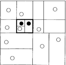
Figure 2.2. “Id-tree data structure. The black dot is the query point, and the
shaded dot is the nearest neighbor. Outside the black box does not need to be searched to find the nearest neighbor.
database, for a naive implementation we need n distance computations. For an efficient implementation, a kd-tree can be employed.
A kd-tree is a binary data structure that recursively splits a A;-dirnensional space into smaller subregions, and those subregions are the branches or leaves of the tree data structure. The search for the nearest neighbors starts from the nearby branches in the tree. For a given distance threshold there is no need to search further branches by implementing this data structure. Figure 2.2 illustrates a two-dimensional region.
2 .3
R e g r e s s io n b y R u le I n d u c tio n
Inducing rules from a given training set is a well-studied topic in machine learning. Weiss and Indurkhya employed rule induction for a regression prob lem and reported significant results [58, 59]. In this section, we will first review the rule-based classification algorithm [57], Swap-1, that learns decision rules in Disjunctive Normal Form (DNF), and later on describe its adaptation for regression.
[1] Input: D, a set of training cases
[2] Initialize Ri <— empty set, /?<— !, and Ci D
[3] repeat
[4] create a rule B with a randomly chosen attribute as its left-hand side [5] while (B is not 100-percent predictive) do
[6] make single best swap for any component of B, including deletion of the component, using cases in Ck
[7] If no swap is found, add the single best component to B [8] endwhile
[9] Pk rule B that is now 100-percent predictive [10] Ek <— cases in C that satisfy the single-best-rule Pk
[11] R k + i^ R k ( J { P k }
[12] Ck+i Ck — {Ek}
[13] k ^ k + 1
[14] until {Ck is empty)
[15] find rule r in Rk that can be deleted without affecting performance on cases in training set D
[16] while (r can be found)
[17] Rk+i ^ R k - {r}
[18] k ^ k - \ - \
[19] endwhile
[20] output Rk and halt.
Figure 2.3. Swap-1 Algorithm
The main advantage of inducing rules in DNF is their explanatory capa bility. It is comparable to decision trees since they can also be converted into DNF models. The most important difference between them is that the rules are not mutually exclusive, as in decision trees. In decision trees, for each instance, there is exactly one rule encoding, a path from a root to a leaf, that is satisfied. Because of this restriction, decision tree models may not produce compact models. However, because of this property of rule-based models, the problem emerges that, for a single instance, two or more classes may be sat isfied. The solution found for this problem is to assign priorities or ordering to the rules according to their extraction order. The first rule, according to this ordering that satisfies the query instance, determines the class of a query. The Swap-1 rule induction algorithm [57] and its sample output are shown in Figure 2.3 and Figure 2.4, respectively.
C A > 0.5 And C P > 3.5 ^ Class = 2 T H A L > 6.5 ^ Class = 2 [True] <— Class = 1
Figure 2.4. A solution induced from a hart-disease data
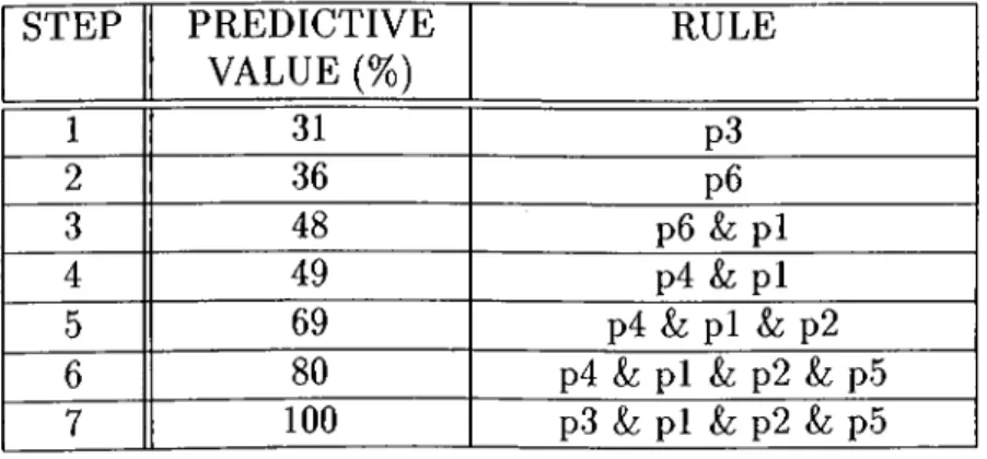
While constructing a rule, the Swap-1 algorithm searches all the conjunctive components it has already formed, and swaps them with all possible compo nents it will build. This search also includes the deletion of some components from the rule. If no improvement is established from these swaps and deletions, then the best component is added to the rule. To find the best component to be added, the predictive value of a component, as the percentage of correct decisions, is evaluated. If the predictive values of them are equal, maximum instance coverage is used as the second criterion. These swappings and addi tions end when the rule reaches 100% prediction accuracy.
STEP PREDICTIVE VALUE(%) RULE 1 31 p3 2 36 p6 3 48 p6 L· pi 4 49 p4 & pi 5 69 p4 &; pi &: p2 6 80 p4 &: pi & p2 & p5 7 100 p3 & pi & p2 & p5 Table 2.1. Example of swapping rule components.
Table 2.1 illustrates a sample rule induction. After forming a new rule for the model, all instances that the rule covers are removed from the instance set, and the remaining instances are considered for the following steps. When a class is covered, the remaining classes are considered, in turn. This process iterates until the instance set becomes empty, that is, all instances are covered.
After formation of the rule set, if the removal of any rule does not change the performance on training set, such rules are removed from the model. Fur thermore, to reach an optimum rule set, an optimization procedure is used [57]. The rule induction algorithms for classification, such as Swap-1, can also be applied to regression problems. Since these algorithms are designed for the
prediction of nominal attributes, using a preprocessing procedure, the numeric attribute in regression to be predicted is transformed to a nominal one.
[1] Input: {y} a set of output values
[2] Initialize n = number of cases, k = number of classes [3] repeat for each Classi
[4] Classi = next n / k cases from list of sorted y values
[5] end
[6] repeat for each Classi (until no change for any class) [7] repeat for each case j in Classi
[8] 1. Move Cascij to Classi-i , compute Er r new [9] If Er r new > Er r old return CaseijtoCi
[10] 2. Move Cascij to Classi^i , compute Er r new [11] If Er r new > Er r old return Cascij to Ci [12] next Cascj in Classi
[13] Next Classi
[14] repeat for each Classi (until no change for any class) [15] If Mean(C'/a5s,·) = Mean(C'/assj) then
[16] Combine Classi and Class] [17] end
Figure 2.5. Composing Pseudo-Classes (P-Class)
For this transformation, the P-class algorithm, shown in Figure 2.5, is used in [59]. This transformation is in fact a one-dimensional clustering of training instances on response variable y, in order to form classes. The purpose is to make y values within one class similar, and across classes dissimilar. The assignment of these values to classes is done in such a way that the distance between each yi and its class mean must be minimum.
The P-Class algorithm does the following. First it sorts the y values, then assigns an approximately equal number of contiguous sorted ?/, to each class. Finally, it moves a j/j to a contiguous class if it reduces the distance of it to the mean of that class.
This procedure is a variation of the K M E A N S clustering algorithm [16, 35]. Given the number of initial clusters, on randomly decomposed clusters, the
1. Generate a set of Pseudo-classes using the P-Class algorithm. 2. Generate a covering rule-set for the transformed classification
problem using a rule induction method such as Swap-1.
3. Initialize the current rule set to be the covering rule set and save it. 4. If the current rule set can be pruned, iteratively do the following:
a) Prune the current rule set.
b) Optimize the pruned rule set and save it.
c) Make this pruned rule set the new current rule set.
5. Use test instances or cross-validation to pick the best of the rule sets.
Figure 2.6. Overview of Method for Learning Regression Rules
K M E A N S algorithm swaps the instances between the clusters if it increases a
clustering measure or criterion that employs inter and intra-cluster distances. Given the number of classes, P-Class is a quick and precise procedure. However, no idea is stated in. the literature about an efficient way to determine the number of classes.
After the formation of classes (pseudo-classes) and the application of a rule induction algorithm to these classes, such as Swap-1, in order to produce an optimum set of regression rules, a pruning and optimization procedure can be applied to these rules, as described in [57, 59]. An overview of the procedure for the induction of regression rules is shown in Figure 2.6.
The naive way to predict the response for a query instance is to assign the average of responses. The average may be a median or mean of that class. However, different approaches also can be considered by applying a paramet ric or non-parametric model for that specific class. For example, the nearest neighbor approach is used for this purpose, and significant improvements of this combination against the naive approach are reported in [59].
2 .4
P r o j e c t io n P u r s u it R e g r e s s io n
One problem with most local averaging techniques, such as the nearest-neighbor, is the curse of dimensionality. If a given amount of data is distributed in a
high-dimensional space, then the distance between adjacent data points in creases with increasing number of dimensions [29]. Friedman and Stuetzle give a numeric example about this problem [20]. Projection pursuit regression (PPR) forms the estimation model by reflecting the training set onto lower dimensional projections as a solution for high dimensional data sets.
Another important characteristic of PPR is its successive refinement prop erty. At each step of model construction, the best approximation of the data is selected and added to the model, while removing the well described portion of the instance space. The search on the data set continues for the I'emain- ing part and this process iterates by increasing the complexity of the model at each step. The successive refinement concept is applied to regression in a different way here, by subtracting the smooth from residuals. A smooth is a function formed by averaging responses (y). An example of smooth is shown in Section 2.4.2.
The model approximated by the PPR algorithm is the sum of the smooth functions S of the linear projections, determined in each iteration:
v(x) = E 5im (/?m .X) (
2
.10
)m = l
where fixa is the parameter vector (projection), X is the training set against predictor variables, is i'h® smooth function and M is the number of terms or smoothes in the model.
2.4.1
P r o je c tio n P u rsu it R eg ressio n A lg o r ith m
At each iteration of the PPR algorithm, a new term, m in Equation 2.10, is added to the regression surface (/?. The critical part of the algorithm is the search for the coefficient vector ¡3 or projection of the next term. After finding a coefficient vector at each iteration, the smooth of the estimated response values resulting from the inner product is added to the model as a new term, where the term is a function of all features. The linear sum of these functions (2.10) forms the model, which is employed for the prediction task.
,n [1] n <- yi , M <- 0, i = I,.
[2] Search for the coefficient vector that maximize fitting criterion I(/3) by using Equation 2.11
[3] If /(/?) is greater than the given threshold [4] Tj' < Tj i 1 , . . . , n ¡5] M ^ M + 1
[6] go to Step 2
[7] Otherwise stop, by excluding last term M.
Figure 2.7. Projection Pursuit Regression Algorithm
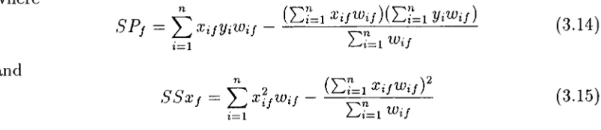
The search for the coefficient vector for each term is done according to a fitting criterion (figure of merit) such that, the average sum of the squared differences between residuals and the smooth is the minimum. For this purpose, /(/3), the fraction of unexplained variance that is explained by smooth Sp, is used as an optimality criterion or figure of merit. I(/3) is computed as
i = l ¿= 1
(
2
.
11
)
where ri is a residual which takes the value of y, in the first step of the algo rithm. The coefficient vector /3 that maximizes I{/3) is the optimal solution.
In the first line of the algorithm current residuals and the term counter are initialized. In the second step, the coefficient vector that results in the best smooth close to the residuals according to the fitting criterion I is found. A smooth is found for each ^ vector, in ascending order of the linear combination (/3.X). If the criterion value found is below a given threshold, the iteration of the algorithm is continued by the new residual vector, which is found by sub tracting the smooth from the current residuals at Step 4. W ith this subtraction operation, the algorithm gains the successive refinement characteristic.
For search of the coefficient vector that maximizes the fitting criterion, a modification of the Rosenbrock method [50] is chosen in [20], and as a smooth ing procedure, a method is described in the next subsection.
Some models approximate the regression as a sum of the functions of in dividual predictors (standard additive models), and because of that, they can
not deal with interactions between predictors. In such models, the projections are done onto individual predictors rather than onto a projection vector, which is the linear sum of the predictors, as in PPR. These projection vectors, instead of individual predictors, allow PPR to deal with interactions, which is the third main property of PPR.
2.4.2
S m o o th in g A lg o r ith m
Traditional smoothing procedures assume that the observed variation, response
yi, is generated by a function which has a normally distributed error compo
nent. The smooth constitutes an estimation for that, function. As an example, in simple linear regression, this function is a linear combination of predictors. As stated above, PPR tries to explain this variation with not just one smooth, but with a sum of smoothes over linear combinations of predictors.
Generally, the smooth functions employed here are not expressions, rather, they are a local averaging of the responses or residuals. Taking the averages of responses in neighborhood regions forms this smooth function. The boundaries of the neighborhood region where the averages are taken are called bandwidth. For example, in the k-nearest neighbor algorithm, k is used for the constant bandwidth. In [20], a variable bandwidth algorithm is employed, where larger bandwidths are used in regions of high local variability of response. To clar ify the concept of smoothing, we describe the constant bandwidth smoothing algorithm of Tukey [52] called “running Medians”.
Running medians is a simple procedure that averages the response by tak ing the median of the neighbor region. Running medians of three algorithms, described in [52], are shown with a simple example in Figure 2.8. The smooth of each response is found by the median of three values in the sequence. One of them is the response itself, and other two are neighbors.
Given : 4 7 9 3 4 11
Smooth : ? 7 7 4 4 11
12 1304 10 15 12 13 17 12 12 15 12 13 13 ? Figure 2.8. Running Medians of Three
Friedman and Stuetzle [20], employ running medians of three in their vari able bandwidth smoothing algorithm, as is shown in Figure 2.9.
[1] Running medians of three;
[2] Estimating the response variability at each point by the average squared residual of a locally linear fit with constant bandwidth;
[3] Smoothing this variance estimates by a fixed bandwidth moving average; [4] Smoothing the sequence obtained by pass (1) by locally linear fits with
bandwidths determined by the smoothed local variance estimates obtained in pass (3).
Figure 2.9. Variable Bandwidth Smoothing Algorithm
In Step 1, a smooth for the response is formed. In Step 2, for each smoothed response value, we find the variance of the neighbors in the interval determined by a given constant bandwidth. In Step 3, these variances are smoothed by a given constant bandwidth. Finally, by employing these smoothed variance values as a bandwidth for each smoothed response determined in Step 1, a variable bandwidth smooth is obtained.
2 .5
R e g r e s s io n b y T ree I n d u c tio n
Tree induction algorithms construct the model by recursively partitioning the data set. The task of constructing a tree is accomplished by employing a search for an attribute to be used for partitioning the data at each node of the tree. The explanation capability of regression trees and their use to determine key features from a large feature set are their major advantages. In terms of performance and accuracy, regression tree applications are comparable to other models. Regression trees are also shown to be strong when there are higher order dependencies among the predictors.
One characteristic common to all regression tree methods is that, they par tition the training set into disjoint regions recursively, where the final partition is determined by the leaf nodes of the regression tree. To avoid overfittiiig and form simpler models, pruning strategies are employed in all regression tree methods.
In the following subsections, three different regression tree methods are de scribed: CART, RETIS and M5. They share the common properties described above, but show significant differences in some of measures and traits they demonstrate.
2.5.1
C A R T
Using trees as regression models was first applied in the CART (Classification and Regression Trees) program, developed by the statistical research commu nity [9]. This program induces both regression and classification trees.
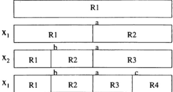
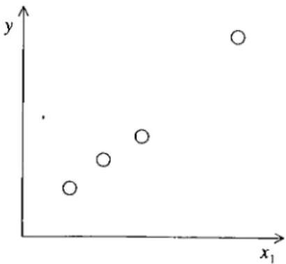
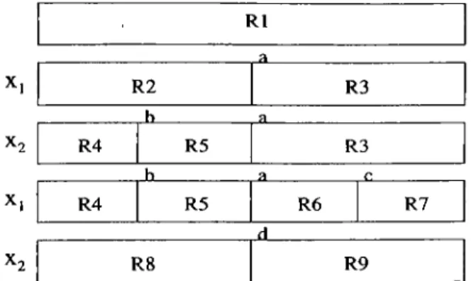
In the first step, we start with the whole training set represented by the root node to construct the tree. A search is done on the features to construct the remaining part of the tree recursively. We find the best feature and feature value of any instance at which to split the training set represented by the root node. This splitting forms two leaf nodes that represent two disjoint regions in the training set. In the second step, one of these regions is selected for further splitting. This splitting is again done according to a selected feature value of an instance. At each step of partitioning, one of the regions, which are not selected before are taken and partitioned to two regions in the same manner along a feature dimension.
After forming regions, which are represented by the leaf nodes of a tree, a constant response value is used for estimation of a query. When a test instance is queried, the leaf node that covers the query location is determined. A constant average value of response values of the instances of the region is assigned as the prediction for the test instance. Each disjoint region has its own estimated value that is assigned to any query instance located in this region.
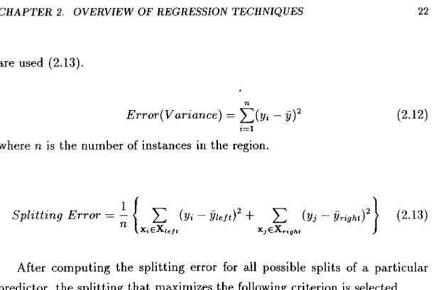
To construct optimum disjoint regions, an error criterion is used. The op timum value of this criterion produces a decomposition at any step of the tree induction process described above so that the correct region, feature, feature value (splitting surface) and estimates for each region are selected. To deter mine the predicted target values in these regions, averaging methods such as mean and median are used. As a fitting criterion, the variances of the regions
are used (2.13).
E r r o r i y ariance) = — yY
t = l
where n is the number of instances in the region.
(2.12)
Splitting Error = ~ l H (Vi “ Hn/tf + J]) (Vj - Vrighif > (2.13) ^XiGXu/t
After computing the splitting error for all possible splits of a particular predictor, the splitting that maximizes the following criterion is selected.
C = Variance — Splitting Error (2.14)
The node and predictor that reach the maximum criterion (7, are selected for splitting. An example regression tree is shown in Figure 2.10. The con struction process is illustrated in Figure 2.11.
Figure 2.10. Example of Regression Tree
Formally, the resulting model can be defined in the following form [9, 19]: If then f { x ) = g r a i x M l ) . (2.15)
Figure 2.11. An example of the tree construction of process. Four regions are determined by predictors a;i and X2·
where {Rm}i a,re disjoint subregions representing p partitions of the training set. The functions g are generally in simple parametric form. The most com mon parametric form is a constant function (2.16), which is illustrated with the example given in Figure 2.10.
(2.16)
The constant values of leaves or partitions are generally determined by averaging. More formally, the model can be denoted by using basis functions:
M rn=l
The basis functions Bm{x) take the form
(2.17)
.B„i(x) = / ( x
e
/ C )(2.18)
where / is cin indicator function having the value one if its argument is true and zero otherwise. Let H[g\ be a step function, indicating a positive argument
m =
1 if 7/ > 0
0 otherwise (2.19)
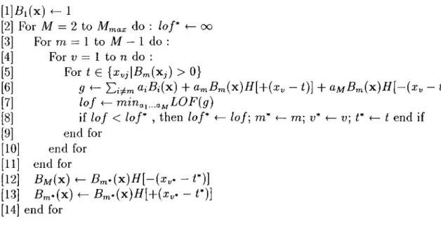
and let LOF(5') be a procedure that computes the lack of fit of an estima tion function g to the data. The recursive partitioning algorithm is given in Figure 2.12.
[1] ^i ( x ) ^ 1 [2] For M = 2 to M„ do : /o/* <— oo [3] [4] [5] [6] [7] [8] [9] [
10
] [11] [12
] [13] For m = 1 to M — 1 do : For = 1 to n do : For t C {Xvj\Bm{y-j) > 0} S < ”1“ <Zm5jrj(x)ii[d'(.Xt; t)] -|- (^Xy 0] lof <- minai...aMLOF{g)if l o f < lof* , then lof* < end for end for end for Bm(^) ^ Bm^i^)H[-{Xy· -t*)] B ^.(x ) <- Bm>iy^)H[+iXy· - t*)] lof·, m* m; u* <— n; i* <— i end if [14] end for
Figure 2.12. Recursive Partitioning Algorithm
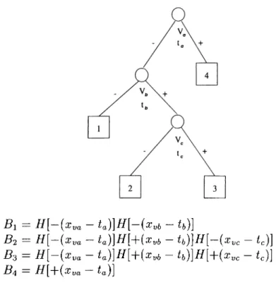
The first line of the algorithm assigns the whole training set as the initial region. The first loop iterates the splitting until reaching a maximum num ber of regions. The next three loops selects the optimum basis function Bm· (intuitively the optimum region), predictor a;,,., and split point t*. At lines 12 and 1.3, the selected region for splitting, Bm-, is replaced with its two parti tions. This is done by adding a factor to its product; with H[—(xy» — /*)] for the negative portion of the region at line 12 by creating a new basis function, and with H[+{xv· — i*)] for the positive portion of the region at line 13, by modifying or removing the previous basis function. Finally the basis functions formed by the algorithm will .take the following form:
A '„
(2.20)
k=l
where the quantity Km is the number of splits that gave rise to Bm, and the arguments of the step functions contain the parameters associated with each of these splits. The quantity Skm takes ( + / —)! values indicating the right/left portions, v{k,m) label the predictor variables, and tkm represent values on the corresponding variables. A possible output of the algorithm is shown in Figure 2.13.
Bi - /{[-(Xya - ia)]B[-(Xyb ~ ¿(,)]
B 2 = B [ - ( X y a - t a ) ] H[ + { Xy b - t b ) ] H[ ~ { X y c ~ ¿ c ) ]
B-i = H [ - { X y a - t a ) ] H[ + { X v b - t b ) ] H[ + { X y c ~ tj)]
B4 = H[-\-(Xya — ia)j
Figure 2.13. A binary tree representing a recursive partitioning regi’ession model with the associated basis functions
The partition may lead to very small regions with a large tree. This sit uation may cause overfitting with unreliable estimates. Stopping the process early may also not produce good results. The solution to this problem is to employ a pruning strategy.
Pruning the regression tree by removing leaves will leave holes, which is an important problem, since we will not be able to give an answer to queries that fall into these regions or holes. That is why the removal of regions is done pairwise, with siblings, by merging them into a single (parent) region. This pruning strategy is described in [9].
Recursive partitioning regression is an adaptive method, one that dynam ically adjusts its strategy to take into account the behavior of a particular problem to be solved [19]. For example, recursive partitioning hcis the ability to exploit low local dimensionality of functions. In local regions, the depen dence of the response may be strong on a few of the predictors, and these few variables may be different in different regions. Another property of recursive partitioning regression is that they allow interpretations, especially when a
constant estimation is done on the leaves.
On the other hand, it has some drawbacks and limitations, the most im portant is the fact that the estimation is discontinuous. The model cannot approximate even simple continuous functions such as linear functions, which limits the accuracy of the model. As a consequence of this limitation, one can not extract from the representation of the model the structure of the function (e.g. linear or additive), or whether it involves a complex interaction among the variables.
2.5.2
R E T IS
In the basic CART algorithm described above, the estimated response value,
y on the leaves of the regression tree was a constant function(2.16). On the
other hand, RETIS (Regression Tree Induction System) [33, 34], a different approach used to construct regression trees, developed by the machine learning community, is an extension of CART that employs a function on the leaves. This is a linear function of continuous predictors. The use of linear regression at the leaves of a regression tree is called local linear regression [33]. RETIS can also be categorized as a LWR system (Section 2.2).
O
O
o
o
Figure 2.14. An example region, with large variance, which is inappropriate for splitting
RETIS is not just a modification of CART at the leaf nodes. The em ployment of linear regression enforces modifications in the construction of the regression tree. In the process of tree construction, the CART system forms subtrees to minimize the expected variance (2.13). However, when applying
local linear regression to a regression tree, the variance is not an appropriate measure as an optimality criterion. If the relationship between the predictors and response is linear, this region may not be appropriate for splitting even if the variance is very large. This situation is illustrated with an example in [3.3]. Suppose we have a region with four instances described with only one predictor as shown in Figure 2.14. Even the error is large in terms of variance, it is almost zero according to a linear approximation on these four points. Such regions cire not appropriate for further splitting. That is why an alternative splitting criterion is employed in RETIS as given in Equation 2.22. Let us first define impurity measure^ I:
/ ( X ) = E ( w - «(>'.))' (
2
.21
)2 = 1
where n is the number of instances, g is the linear function that best fits the instances of the region. Consequently, the figure of merit (the splitting criterion) is defined as in Equation 2.22.
^ T ^^rightJ^right\ (2.22)
The use of Equation 2.21 instead of Equation 2.13 in computing figure of merit is the main difference between CART and RETIS. When estimating a response value for a query, the value that results from the linear function on which the leaf node the query falls is used.
After construction of a regression tree, a pruning strategy is employed, as in most other tree induction models. See [41] for an in-depth explanation of pruning. The strategy used in RETIS computes two different error measures:
static error and the backed-up error. The static error is computed at a node,
supposing it is a leaf, and backed-up error is computed at the same node for the ca,se, in which the subtree is not pruned. If the static error is less than or equal to the backed-up error, then the subtree is pruned at that node, and the tree node is converted into a leaf node.
2 .5 .3
M 5
M5 is another system [45] that builds tree-based models for the regression task, similar to CART and RETIS. Although the tree construction in M5 is similar to CART, the advantage of M5 over CART is that the trees generated M5 are generally much smaller than regression trees. Standard deviation is employed as the error criterion in M5, instead of variance as used in CART. The reduction on the error (2.23) on subregions after splitting a region is the measure used to decide on splitting:
error = <^(x) - E (2.23)
where cr is standard deviation and i is the number of subregions of a region whose instances are denoted by X. After examining all possible splits, M5 chooses the one that maximizes the expected error reduction (2.23).
M5 is also similar to RETIS in that it employs a linear regression model on the nodes to estimate responses by using standard linear regression tech niques [43]. These linear models are constructed on all the nodes, starting from the root down to the leaves. However, instead of using all the attributes or predictors, a model at a node is restricted to the attributes referenced by linear models in the subtree of that node.
After constructing the tree and forming linear models at the nodes as de scribed above, each model is simplified by eliminating parameters to maximize its accuracy. The elimination of parameters generally causes an increase in the average residual. To obtain linear models with fewer of parameters, the value is multiplied by (n -f p){n — p), where n is the number of instances and p is the number of parameters in the model. The effect is to increase the estimated error of models with many parameters and with a small number of instances or training cases. M5 uses a greedy search to remove variables that contribute little to the model. In some cases, M5 removes all of the variables, leaving only a constant [33].
The pruning process in M5 is the same as RETIS. To prune the constructed tree, each non-leaf node is examined, starting near the bottom. If the estimated