Linear planning logic and linear logic graph planner: domain independent task planners based on linear logic

(1)

LINEAR PLANNING LOGIC AND LINEAR

LOGIC GRAPH PLANNER: DOMAIN

INDEPENDENT TASK PLANNERS BASED

ON LINEAR LOGIC

a dissertation submitted to

the graduate school of engineering and science

of bilkent university

in partial fulfillment of the requirements for

the degree of

doctor of philosophy

in

computer engineering

By

Sıtar Kortik

September, 2017

(2)

Linear Planning Logic and Linear Logic Graph Planner: Domain Independent Task Planners Based On Linear Logic

By Sıtar Kortik September, 2017

We certify that we have read this dissertation and that in our opinion it is fully adequate, in scope and in quality, as a dissertation for the degree of Doctor of Philosophy.

Varol Akman(Advisor)

Ulu¸c Saranlı(Co-Advisor)

Pınar Karag¨oz

U˘gur G¨ud¨ukbay

¨

Ozg¨ur Ulusoy

Faruk Polat

Approved for the Graduate School of Engineering and Science:

Ezhan Kara¸san

(3)

ABSTRACT

LINEAR PLANNING LOGIC AND LINEAR LOGIC

GRAPH PLANNER: DOMAIN INDEPENDENT TASK

PLANNERS BASED ON LINEAR LOGIC

Sıtar Kortik

Ph.D. in Computer Engineering Advisor: Varol Akman Co-Advisor: Ulu¸c Saranlı

September, 2017

Linear Logic is a non-monotonic logic, with semantics that enforce single-use assumptions thereby allowing native and efficient encoding of domains with dy-namic state. Robotic task planning is an important example for such domains, wherein both physical and informational components of a robot’s state exhibit non-monotonic properties. We introduce two novel and efficient theorem provers for automated construction of proofs for an exponential multiplicative fragment of linear logic to encode deterministic STRIPS planning problems in general. The first planner we introduce is Linear Planning Logic (LPL), which is based on the backchaining principle commonly used for constructing logic programming languages such as Prolog and Lolli, with a novel extension for LPL to handle program formulae with non-atomic conclusions. We demonstrate an experimen-tal application of LPL in the context of a robotic task planner, implementing visually guided autonomous navigation for the RHex hexapod robot. The sec-ond planner we introduce is the Linear Logic Graph Planner (LinGraph), an automated planner for deterministic, concurrent domains, formulated as a graph-based theorem prover for a propositional fragment of intuitionistic linear logic. The new graph-based theorem prover we introduce in this context substantially improves planning performance by reducing proof permutations that are irrele-vant to planning problems particularly in the presence of large numbers of objects and agents with identical properties (e.g. robots within a swarm, or parts in a large factory). We illustrate LinGraph’s application for planning the actions of robots within a concurrent manufacturing domain and provide comparisons with four existing automated planners, BlackBox, Symba-2, Metis and the Tempo-ral Fast Downward (TFD), covering a wide range of state-of-the-art automated planning techniques and implementations that are well-known in the literature for their performance on various of problem types and domains. We show that even

(4)

iv

though LinGraph does not rely on any heuristics, it still outperforms these sys-tems for concurrent domains with large numbers of identical objects and agents, finding feasible plans that they cannot identify. These gains persist even when existing methods on symmetry reduction and numerical fluents are used, with LinGraph capable of handling problems with thousands of objects. Following these results, we also formally show that plan construction with LinGraph is equivalent to multiset rewriting systems, establishing a formal relation between LinGraph and intuitionistic linear logic.

Keywords: Automated planning, Linear logic, Multiset rewriting, Automated theorem prover.

(5)

¨

OZET

DO ˘

GRUSAL PLANLAMA MANTI ˘

GI VE DO ˘

GRUSAL

MANTIK GRAF˙IK PLANLAYICI: DO ˘

GRUSAL

MANTIK TABANLI ALAN BA ˘

GIMSIZ G ¨

OREV

PLANLAYICILAR

Sıtar Kortik

Bilgisayar M¨uhendisli˘gi, Doktora Tez Danı¸smanı: Varol Akman ˙Ikinci Tez Danı¸smanı: Ulu¸c Saranlı

Eyl¨ul, 2017

Do˘grusal mantık, tek kullanımlık varsayımları kullanmaya zorlayan tekd¨uze

ol-mayan bir mantık oldu˘gu i¸cin, dinamik durumlu alanları etkili olarak g¨ostermeye

olanak sa˘glıyor. ˙I¸cinde, bir robotun durumunda fiziksel ve bilgisel bile¸senlerin bir-likte tekdüze olmayan özellikler sergilendi˘gi robotik görev planlaması, bu tür alan-lar i¸cin önemli bir örnektir. STRIPS planlama problemleri i¸cin, do˘grusal mantıkta ispatları otomatik ortaya ¸cıkaracak iki adet yeni ve etkili teorem ispatlayıcı

or-taya koyuyoruz. Ortaya koydu˘gumuz ilk planlayıcı olan Do˘grusal Planlama

Mantı˘gı, Prolog ve Lolli gibi programlama dillerinde sık¸ca kullanılan geriye zincir-leme prensibiyle ¸calı¸smaktadır ve atomik olmayan sonu¸cları da ele alacak ¸sekilde geni¸sletilmi¸stir. Bu yeni planlayıcının deneysel bir uygulaması olan RHex robotu i¸cin görsel yönlendirmeyle otomatik gezinme, robotik görev planlayıcı kapsamında gösterilmi¸stir. Ortaya koydu˘gumuz ikinci planlayıcı olan Do˘grusal Mantık Grafik Planlayıcısı, do˘grusal mantık i¸cin grafik tabanlı teorem ispaylayıcı olarak formüle edilmis, rastgele olmayan ve e¸s zamanlı alanlar icin otomatik bir planlayıcıdır. Bu yeni grafik tabanlı teori ispatlayıcı, ¸coklu sayıdaki özde¸s nesnelerin oldu˘gu zamanlarda (sürü icindeki robotlar, büyük fabrikadaki par¸calar), özellikler

plan-lama problemleriyle alakası olmayan ispat perm¨utasyonlarını azaltarak planlama

performansını arttırıyor. ˙Ikinci planlayıcının, e¸s zamanlı ¨uretim alanında eylem

planlaması icin uygulamasını örnek üzerinde gösteriyoruz ve literatürde farklı

problem tiplerinde ve alanlarında performanslarıyla bilinen, d¨ort farklı otomatik

planlayıcı olan BlackBox, Symba-2, Metis ve Temporal Fast Downward (TFD) ile karsıla¸stırmasını sa˘glıyoruz. Yeni planlayıcımızın herhangi bir bulu¸ssala ba˘glı olmamasına ra˘gmen, di˘ger sistemleri ¸coklu ¨ozde¸s nesnelerin varlı˘gında e¸s zamanlı alanlarda yendi˘gini g¨osteriyoruz. Simetri azaltma ve sayısal akı¸skanlar ile ilgili

(6)

vi

mevcut metodlar kullanılsa bile, yukarıdaki kazanımlar s¨ur¨uyor ve yeni

plan-layıcımız binlerce nesneli problemleri ¸c¨ozebiliyor. Bu ¸cıkarımlara ek olarak, bu

yeni planlayıcı ile plan olu¸sturmanın, ¸coklu k¨ume yeniden yazım sistemlerine e¸sit oldu˘gunu g¨osteriyoruz.

Anahtar sözcükler : Otomatik planlama, Do˘grusal mantık, Ç oklu küme yeniden

(7)

Acknowledgement

I thank my advisor Ulu¸c Saranlı for helping me develop and finish this thesis. His vision, knowledge and creativity carried me forward to this day.

I also thank my advisor Varol Akman for being with me from beginning of my MS thesis until this day. His advises and guidance gave me strength throughout these years.

This work would not have been possible without supervision of Frank Pfenning, whose collaboration and advice helped me coming up with the idea of LinGraph during my visit to the Carnegie Mellon University.

I thank my thesis committee, Pınar Karagöz, U˘gur Güdükbay, Özgür Ulusoy and Faruk Polat for their support and giving advice for this thesis.

Many people directly or indirectly contributed to my completion of this the-sis. I thank the Middle East Technical University Couple Dances Club and all of its members for creating the wonderful social setting in which I have discovered my passion for tango. I thank TUBITAK, the Scientific and Technical Research Council of Turkey for their financial support during my visiting of Carnegie Mel-lon University. I am also thankful to the Computer Engineering Department of Bilkent University for their financial support during my PhD studies.

I owe my deepest gratitude to my parents and my sister for their endless love supported me through many years of separation.

(8)

List of Figures

2.1 Proof rules for multiplicative connectives. . . 16

2.2 Proof rules for additive connectives . . . 17

2.3 Proof rules for quantifiers . . . 18

2.4 Proof rules for exponentials . . . 18

2.5 Hypotheses . . . 18

2.6 Predicates and actions for the blocks world planning domain. . . . 19

2.7 Encodings of blocks world planning domain actions in linear logic. 19 3.1 Resolution rules for the linear context and the intuitionistic context. 27 3.2 Multiplicative right sequent rules for the BL proof theory. . . 31

3.3 Exponential and quantifier right sequent rules for the BL proof theory. . . 32

3.4 Resolution rules for atomic goals within the LPL backchaining proof theory . . . 33

3.5 Residuation rules for atomic goals within the LPL backchaining proof theory . . . 35

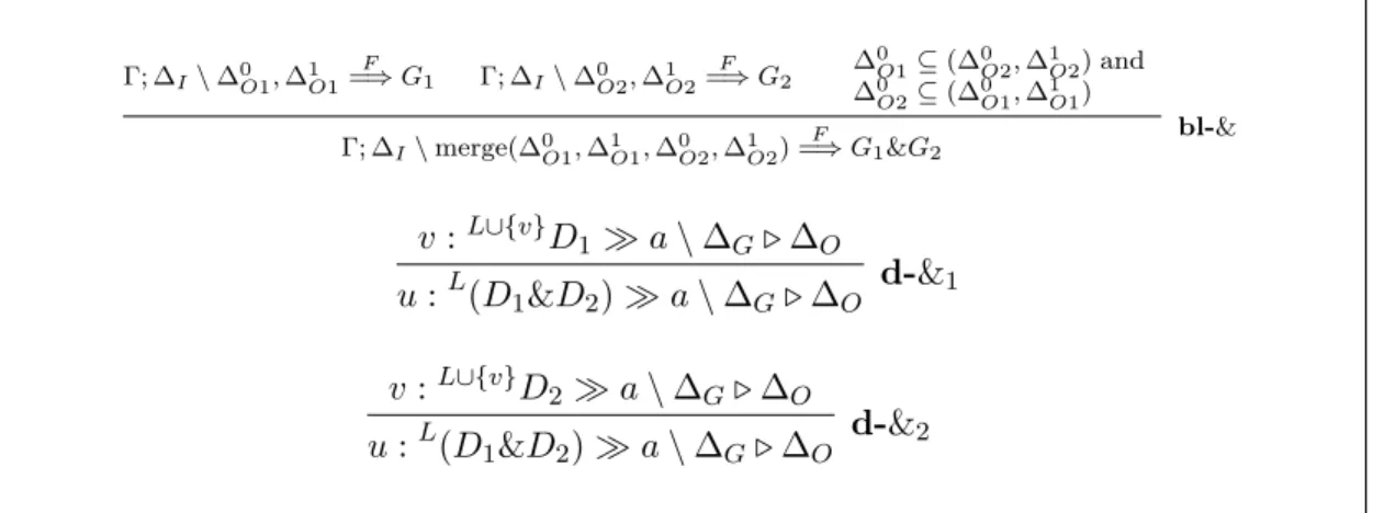
3.6 The alternative conjunction (&) rules for the BL proof theory. . . 36

3.7 Predicates and actions for the robotic planning domain. . . 38

3.8 Encodings of walking and tagging actions within LPL. . . 39

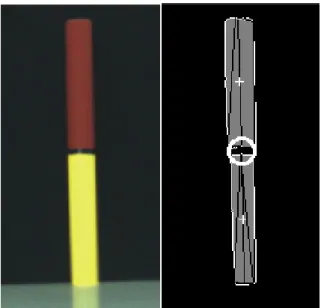
3.9 A snapshot from the experimental setup in its initial state. Six colored landmarks are scattered throughout the environment, ob-servable through a camera mounted on the RHex robot. . . 39

(12)

LIST OF FIGURES xii

3.10 Left: A red-yellow landmark as seen by the robot. Right: blobs extracted from the image with their centers marked with a “+”

sign. Computed landmark location is the midpoint of the two

blobs and is marked with a white circle. . . 41

3.11 Snapshots during the execution of the behavioral plan for RHex

generated by the LPL theorem prover. . . 42

3.12 Objects, states and actions of the mail delivery example. . . 46

3.13 Encodings of the mail delivery actions in LPL. . . 46

3.14 Incorrect proof attempt using first the ⊗R rule, then the ⊗L rule. 47

3.15 Correct proof using the ⊗L rule first, then the ⊗R rule. . . 48

4.1 System RL: A reference sequent calculus system for the LPL

frag-ment of intuitionistic linear logic. . . 51

4.2 Reduction rules with proof annotations for the BL proof theory. . 54

4.3 Resolution and residuation rules with proof annotations for the

BL proof theory. . . 55

4.4 Proof Rewriting procedure. . . 56

4.5 System IL: Initial and left sequent calculus rules. . . 57

4.6 _{Rewriting rules for proofs ending with il- ( L, preceded by il-⊗L}01

or il-⊗L00 on the subgoal (left) branch. . . 80

5.1 Sequent calculus proof rules for LGP L. . . 84

5.2 Objects types and notation for the robotic assembly planning

do-main. . . 86

5.3 An overview of the algorithm for plan search through incremental

construction of a LinGraph instance. . . 90

5.4 Visualization of LinGraph nodes for states, actions and goals,

dis-tinguished by their shapes. Each node shows its corresponding

LGPL formula, the number of its instances n and its unique label. 91

5.5 Visualization of the LinGraph following the creation of nodes for

the initial state and the goal for the planning problem of (5.10). This figure also illustrates initial constraints and the first goal check

(13)

LIST OF FIGURES xiii

5.6 LinGraph expansion example illustrating second level nodes

cre-ated both through copying (s3 and s4) from the first level as well

as the application of a new instance of the MakeP action (s5 and

s6). . . 95

5.7 Final state of the LinGraph for the planning problem of (5.10),

showing all constraints used for the last successful goal check step

with all goals satisfied. . . 97

5.8 LinGraph expansion step checking for feasibility of a new instance

of the MakeP action through action constraints. . . 100

5.9 Plan extraction using the solution obtained from the constraint

solver. Each state node shows the number of utilized resources in the lower right corner. Unused state nodes are faded out for clarity. 101 5.10 Solution to the modified planning problem of (5.12) . . . 101

5.11 Objects and actions encoding of the real world planning example. 105

5.12 Linear logical encodings of actions within the more complex as-sembly planning problem domain. . . 105 5.13 Final LinGraph for the complex assembly planning example of

(5.13). Some actions and nodes for levels larger than 2 were omit-ted for visual clarity. Nodes that are part of the final plan are shown in red. . . 106 5.14 Solution to the complex assembly planning problem defined by (5.13)107 5.15 Encodings of actions for Domain-1 in LGPL. . . 109 5.16 PDDL domain file encoding Domain-1, an assembly planning

ex-ample with two types of components. . . 109 5.17 Encoding the problem with four components for Domain-1 in PDDL.110 5.18 PDDL encoding of the durative version of the MakeS1 action for

Domain-1 . . . 111 5.19 PDDL encoding of Domain-1 using numerical fluents to capture

object multiplicity. This figure only shows the definition of the MakeS1 action . . . 112 5.20 An example PDDL problem definition for Domain-1 using

numer-ical fluents, featuring six manipulators to produce a total of three products . . . 112

(14)

LIST OF FIGURES xiv

5.21 New action definition in the PDDL domain file encoding of Domain-2. . . 117 5.22 The cooperative multi-robot domain consisting of two supply

sta-tions, l1 and l2 and a base station l0. This figure also illustrates

the initial state for our examples, wherein 2n wheels, n body parts and r robots are available in their corresponding stations. Arrows indicate connections between locations traversable by robots. . . . 119 5.23 LGPL encoding of the example for cooperative multi-robot

assem-bly of bicycles. Propositions encoding components of the state, together with LGPL action definitions and their descriptions are

given. . . 120

5.24 The desired final state for the example multi-robot cooperative assembly domain. n fully assembled bicycles and r robots should be located in the base station l0. . . 121

5.25 Solution to the multi-robot example encoded by (5.20) with n = 1

and r = 7, generated by the LinGraph planner. . . 121

(15)

List of Tables

5.1 Execution times (in seconds) for Domain-1 with twice the number

of initially available manipulators as the number of initial compo-nents n. LinGraph solutions have 4 levels . . . 113

5.2 Execution times (in seconds) for Domain-1 with the same number

n of initially available components and manipulators. LinGraph

solutions have 4 levels . . . 114

5.3 Execution times (in seconds) for Domain-1 with the number m

of initially available manipulators a non-integer multiple of the number n of initially available components. LinGraph solutions have 4 levels . . . 114

5.4 LinGraph level, node and constraint statistics for different

in-stances of the planning problem in (5.17). . . 115

5.5 Node and constraint statistics for each level of the LinGraph

so-lution for a Domain-1 problem instance with n = 10000 and

m = 10000. . . 115

5.6 Execution times (in seconds) for the problem of (5.18). LinGraph

plans have 4 levels . . . 117

5.7 Execution times (in seconds) for the problem of (5.19). LinGraph

plans have 4 levels . . . 118

5.8 Created nodes and constraints at each level for the Rhex example

(16)

LIST OF TABLES xvi

5.9 Execution times (in seconds) for different planners in solving

in-creasingly large instances of the planning problem encoded by (5.20). LinGraph extends to level 6 in all cases, corresponding to 5 steps. Other planners are unable to solve any of the problem instances . . . 122 5.10 Execution times (in seconds) for different planners on the planning

problem of (5.20) with fewer manipulators. LinGraph extends to level 10 in all cases (9 steps). Other planners abort with errors beyond a certain problem size . . . 122

(17)

Chapter 1 Introduction

1.1 Motivation and Scope

In 1996, Pathfinder successfully landed to the surface of Mars. After landing to the surface, the rover traveled about 100 meters during its 90 day lifetime, more than half of which was spent doing nothing due to plan failure caused by unpredictabilities of resources and other environmental factors while the execu-tion of a given plan [1, 2]. It was not easy to intervene the rover in the existence of a plan failure because of the communication delay between Earth and Mars. Remotely controlling the rover was also very difficult with the same reason. In-stead of teleoperation, for each day operators were sending an one-day plan at once such that moving from one location to another or analyzing the surface of Mars. Subsequently, the rover would run the plan sent previous day [3]. A typ-ical one-day plan included approximately 100 actions, which is very long to be executed without any failures. Unfortunately, during the execution of a given plan, there are many uncertainties such as the power required, the duration of each action, the position and orientation of the rover and other environmental factors like dust on solar panels, etc [4]. A rover capable of fully autonomous de-cision making could have overcome most of these issues. The last rover on Mars, Curiosity [5], has an autonomous navigation mode. However, even this dexterous

(18)

rover depends on operators on Earth. We can hence say that autonomy for mo-bile robotic platforms is a difficult, but important challenge. In the near future, it will be possible to see fully autonomous cars on roads and robot assistants in houses. Such autonomous platforms need planners which can effectively and accurately represent the problem domain and make efficient decisions to achieve given real world goals. One of our motivations is the need for such automated and domain-independent planners.

In this context, we focus on task planning (a.k.a. action planning) [6–8]. Task planning is the problem of selecting an ordered list of actions, starting with a set of possible initial states, to achieve a particular goal state. Physical behavior of a particular system associated with an action is summarized through a list of preconditions and a list of effects for the action, providing a discrete abstraction of system behavior. To be able to use an action, all preconditions must be satisfied. When an action is used, the environment is modified to satisfy the effects of the action. This conceptual framework assumes a discretized view of time. Task planning seeks a plan through these abstract behaviors, manipulating the system from its initial state to the desired final state. The final plan is either a partial or total order of selected actions [9].

Automatic task planning has been among important problems in Artificial In-telligence, with numerous applications in robotics, scheduling, resource planning and even automated programming. Different approaches have been proposed to represent and solve task planning problems. Among these methods, linear logic [10, 11] has been proposed in the literature, capable of handling real world planning problems [12], since linear logic allows native support for representing dynamic state as single-use (or consumable) resources. Consumable resource rep-resentation in linear logic stands in contrast to fact reprep-resentation in classical logic that can be used multiple times or not at all. Together with consumable resources, linear logic can also represent persistent resources that can be used infinitely many times whenever they are needed. Resource representation of lin-ear logic is capable of effectively addressing the well-known frame problem that often occurs in embeddings of planning problems within logical formalisms such as situation calculus [13–16]. Briefly, the frame problem is the need and challenge

(19)

of representing possibly irrelevant non-effects of an action in addition to its more relevant effects.

Our main motivation in this thesis is the exploration of logical approaches with theorem proving for task planning. Unfortunately, using logical reasoning methods and theorem provers in task planning generally runs into complexity issues because of the multitude of valid proofs (all corresponding to the same plan) for the same problem. This fact causes nondeterminism beyond what is inherent in the problem domain itself, and makes the search problem much more difficult [17]. Addressing this issue and introducing an expressive and efficient task planner is challenging. Most research efforts either simplify the representational language, hence sacrificing expressivity, or impose a particular structure on proof search that might impair soundness and completeness of the logic [18].

In this thesis, we propose two different languages and associated theorem provers for task planning using linear logic. The first language that we intro-duce is Linear Planning Logic (LPL), which extends on Linear Hereditary Har-rop formulas (LHHF) that underlie linear logic programming languages such as Lolli [19]. LPL provides increased expressivity compared to Lolli, while manag-ing to similarly keep out-of-domain nondeterminism to a minimum. Expressivity is increased by allowing negative occurrences of conjunction, which as necessary to represent multiple simultaneous preconditions for an action. Adding negative occurrences of conjunction while still preserving a backchaining method for proof search is problematic for linear logic. The proof theory that we propose for this language preserves the deterministic back-chaining structure of provers designed for LHHF. To show expressivity and feasibility of our planning formalism, we illustrate an experimental application for a hexapod robot RHex [20], navigating in an environment populated with visual landmarks.

Our second proposed language for automated generation of plans for STRIPS-based [21] planning problems is Linear Logic Graph Planner (LinGraph), which is a graph-based theorem prover for a multiplicative exponential fragment of propositional linear logic. LinGraph reduces nondeterminism particularly in the

(20)

presence of large numbers of functionally identical resources and agents. We intro-duce a number of different planning domains such as manufacturing to illustrate the application of LinGraph for planning the actions of agents. We also compare LinGraph to four modern planners, four existing automated planners, BlackBox, Symba-2, Metis and the Temporal Fast Downward (TFD), covering a wide range of state-of-the-art automated planning techniques and implementations that are well-known in the literature for their performance on various of problem types and domains.. We show that for specific domains where there are large numbers of identical objects and agents, LinGraph can outperform these systems, finding feasible plans that they cannot identify.

(21)

1.2 Contributions

In this section, we summarize main contributions of the thesis in two categories. For each category, we itemize and summarize individual contributions.

1.2.1 Linear Planning Logic (LPL)

• Introducing a novel logic language and theorem prover:

One of the main contributions of this thesis is introducing a novel logic language and an associated theorem prover for task planning. We call our new language Linear Planning Logic (LPL), consisting of a fragment of linear logic well suited for representing dynamic states and constructing automatic plans efficiently.

• Extending the expressivity of Linear Hereditary Harrop Formulas (LHHF): LPL extends on the expressivity of Linear Hereditary Harrop Formulas (LHHF) by adding negative occurrences of conjunction, allowing actions to create multiple resources.

• Implementing LPL in SWI-Prolog:

In order to show performance of LPL, we implemented it in SWI-Prolog. • Introducing a new robotic planning domain example:

To test the implementation and show the expressivity of LPL, we intro-duced a new robotic planning domain example and encoded a number of example planning problems in LPL. We have shown both the correctness and performance of our LPL theorem prover for this domain.

• Using LPL to construct plans for the hexapod platform RHex

After showing the expressivity of LPL on simple planning domains, we used the hexapod platform RHex for an experimental demonstration of its use.

(22)

1.2.2 Linear Logic Graph Planner (LinGraph)

• Introducing a graph-based theorem prover for task planning:

The second main contribution of this thesis is introducing a graph based theorem prover for task planning, within a propositional fragment of linear logic. We call this framework Linear Logic Graph Planner (LinGraph). • Implementing LinGraph in SML:

We implemented a prototype of LinGraph in SML to compare its perfor-mance with other planners.

• Introducing additional new planning domain examples:

To show expressivity of LinGraph, we introduced additional planning do-main examples and encoded these dodo-mains in our implementation.

• Comparing the performance of LinGraph with other planners:

Another contribution of this thesis is comparing the performance of Lin-Graph with other modern planners, including BlackBox, Symba-2, Metis and the Temporal Fast Downward (TFD) and showing that LinGraph out-performs other planners for certain planning domains in the presence of large numbers of identical objects and agents.

• Establishing a formal relation between LinGraph and linear logic:

We also formally show that plan construction with LinGraph is equivalent to multiset rewriting systems, establishing a formal relation between LinGraph and intuitionistic linear logic.

(23)

1.3 Organization of the Thesis

We will begin by reviewing related literature in Chapter 2, followed by a defini-tion of the fragment of Linear Logic we use for encoding planning problems in Chapter 3. We then present soundness proof of LPL in Chapter 4. In Chapter 5, we introduce LinGraph and an assembly planning domain to present a detailed description of our method, followed by conclusion and future work in Chapter 6.

(24)

Chapter 2 Background and Related Work

2.1 Task (Action) Planning

Task, or action planning is finding an ordered sequence of actions (also called a plan), which will take an agent from a set of possible initial states to a par-ticular goal state. Automation of finding such plans has been among important problems in Artificial Intelligence and can be used for numerous applications in robotics, scheduling, resource planning and even automated programming. Many successful automated planners are based on a discretized view of task planning, which are based on composing continues, low-level behavioral primitives through their high-level abstractions. This structure has been as a basis for numerous languages and methods. Among these, the STRIPS language [21] is one of the most basic but fundamentally useful modeling languages. More capable alterna-tives to STRIPS such as ADL [22, 23] and the more recent PDDL [24] eliminate these limitations and recover substantial expressivity. However, the majority of real-world implementations of automated planners still rely on internal transla-tions to a STRIPS representation, that are exponential in complexity and hence do not eliminate nondeterministic components inherent in the planning problem itself.

(25)

We can categorize automated task planning systems according to the configura-bility of the planner to work in different planning domains [25]. As such, we can talk about domain-specific, domain-independent and domain-configurable plan-ners. Among these, domain independent planners are those that are capable of working in any problem domain. Domain-independent planners [26] have mainly two varieties, state-space and plan-space planners. However, this categorization may not be enough to cover and denote all relevant properties of a planning system. Another categorization could be according to the step-optimality of a planner. Within this classification, our research focuses on domain-independent and step-optimal planning.

Among existing planners, partial-order planning (POP) implements plan-space search rather than state-space search, and eliminates unnecessary nondetermin-ism in the search for plan search originating from irrelevant total orderings of ac-tion sequences [27]. The Universal Condiac-tional Partial Order Planner (UCPOP) method [28] is an important variation of POP and achieves greater expressivity by allowing actions that have variables, conditional effects, disjunctive preconditions and universal quantification. One of more recent optimal planners for STRIPS problems is GraphPlan. Even though GraphPlan has reduced expressivity, it is a practical alternative to UCPOP with better performance [29]. A number of recent extensions and improvements for GraphPlan were been introduced in the literature. In [30], the authors try to combine the expressivity of UCPOP with the efficiency of GraphPlan by transforming domains in UCPOP to their equivalent in GraphPlan. In [31], GraphPlan is extended to contingent planning problems incorporating uncertainty and sensing actions. In [32], the authors ex-plore the use of GraphPlan for probabilistic planning, with a known world but probabilistic actions. A number of introduced planners support nondeterministic actions using GraphPlan’s features. One of such planners is the Fast, Iterative Planner (FIP), illustrated for a simple omelette problem [33]. It has been ca-pable of outperforming other planners, including the model-based MBP system [34] for nondeterministic domains in certain cases. In [35], the authors extend the classic GraphPlan algorithm to support dynamic creation and destruction of objects through new operators specifically introduced for this purpose. Another

(26)

method formulates planning problems as Constraint Satisfaction Problems (CSP) instances [36], claiming that this structure subsumes the representation induced by GraphPlan and leads to a more efficient planner. This also relies on imposing a bound on the length of the plan, reducing search complexity to NP.

Among most successful recent modern optimal task planners, Blackbox [37, 38] and SatPlan implementations [38–41] convert problems specified in STRIPS nota-tion into satisfiability problems. Formulating planning as a satisfiability problem has been introduced by [42], where the central idea is to translate the planning problem into a finite collection of axioms, whose satisfaction corresponds to the solution.

Even though these planners are among the most successful optimal task plan-ners, their plan search complexity is NP-hard [43]. Modern planners based on heuristic search planning (HSP) address this issue of complexity by using a re-laxed problem, which ignores negative effects of actions and resulting mutexes, to compute the heuristic [44–46]. However, these planners based on HSP sacri-fice optimality for efficiency. One of the well-known planners based on this idea is Fast-Forward (FF) planner [47]. A more recent state of the art non-optimal planner is Madagascar [48, 49], capable of quickly finding feasible plans. Another alternative approach for non-optimal planning is using a hierarchical structure for plan search. Hierarchical Task Network (HTN) planning [50, 51] is based on this approach. Initially a high-level task network consists of initial and final states, with high-level abstract tasks, which are then iteratively decomposed until primitive actions are reached.

Another, preceding these modern planners, earlier approaches to task planning used deductive reasoning and theorem proving. However these methods lost their popularity in recent decades, since nondeterministic choices introduced by logi-cal encodings of problem domains often increase the computational complexity of plan search as exemplified by classical logic encodings. Representing dynamic states is also problematic in classical logic. For example, situation calculus at-tempts to represent dynamic states within a planning problem [52] but it suffers from the frame problem, resulting in substantially increased complexity [53].

(27)

In this context, linear Logic [10, 11] is an effective solution to the frame prob-lem, allowing native modeling of dynamic states as single-use (consumable) re-sources within the language itself. Hereby, linear logic eliminates the complexity cost associated with complex solutions to the frame problem [15, 16, 54]. Linear logic’s non-monotonic reasoning in solving the frame problem was also used in other planners, using logic programming and answer sets [14, 55–57]. When using linear logic to encode and solve planning problems, we can compose states using the simultaneous conjunction operator, represent actions with the linear implica-tion connective and model nondeterministic effects with the additive disjuncimplica-tion connective [12, 17, 58, 59]. Linear logic can also model concurrency as explored in [60, 61]. Even though linear logic has these appealing properties, construction of efficient linear logic theorem provers having these properties has been challeng-ing. One of the main issues arises from the logical nondeterminism, introduced by explicit encodings of planning problems through the use of logical connectives. A number of theorem provers such as Lolli restrict the expressivity of the logical language to increase efficiency [19].

Petri Nets can successfully represent concurrent processes and have semantic connections to linear logic [62–65]. The PetriPlan system uses this connection and transforms the planning problem into a reachability query in an acyclic Petri Net, and then uses Integer Programming to find a valid solution.

Another technique for task planning is to use model-based reasoning [34]. In this method, plan construction to solve planning problems is transferred into the problem of searching through a logical semantic structure, without being connected to an explicit proof theory. One of the popular applications of this idea is the use of temporal logic [18]. This method abstractly represents continuous behaviors as atomic propositions and models temporal components through the evaluation of a finite state machine. However, some properties of this method such as its dependence on temporal logic, model checking and abstraction of the physical world decrease expressivity and do not allow deductive reasoning.

(28)

We can use a working domain-independent planner to solve the planning prob-lem in different environments and domains such as manipulation planning, assem-bly line planning and mobile robot planning. The manipulation planning problem usually includes a manipulator robot which interacts with an object, grasping and moving the object to another location in the environment. Among most efficient control architectures for robot manipulators, behavior-based methods stand out for practical applications. However behavior-based methods either require infea-sible computation time or do not ensure completeness. To solve these problems, in [66] the authors present an algorithm for manipulation planning. This algo-rithm plans paths in configuration spaces with multiple constraints such as torque limits, constraints on the pose of an object held by a robot, and constraints for fol-lowing workspace surfaces. Another manipulation planning method is presented in [67], where the authors introduce a formal tool which they call the motion grammar, for task decomposition and hybrid control. This work is interesting in issue of a context free grammar for manipulation planning. They test this formal tool on a chess game with a manipulator robot.

Another application area of robotic planning is assembly line planning. In [68], the author addresses the problem of designing a distributed, hybrid factory given a description of an assembly process and a palette of controllers for basic assembly operations. Another important point of this work is incorporating petri nets into the planning system.

Finally, we briefly mention an existing drawback of efficiency issues in plan-ning, loop, non terminating proof search while constructing a plan. To prevent loops, we need a loop detection and a loop preventing mechanism. In [69], the authors provide a loop detection mechanism for propositional affine logic adapt-ing the history techniques used for intuitionistic logic. This work is good for understanding the loop detection mechanism and how it is used in linear logic. Although loops in proof search may cause efficiency issues, in some cases loops can be necessary in planning. In [70] and [71], a different approach for planning is introduced, where they use loops in planning to deal with an unknown and unbounded planning parameter.

(29)

2.2 Intuitionistic Linear Logic: Language and

Proof Theory

In this section, we present the basic ideas and principles underlying intuition-istic linear logic and show its expressivity on a well-known planning example, the blocks world. Linear logic was first introduced by Girard [10] as a reasoning language that rejects the contraction and weakening rules. Linear logic can be considered both in intuitionistic and classical formulations. In this thesis, we focus on intuitionistic linear logic, since proofs in intuitionistic languages corre-spond to executable programs as formalized by the Curry-Howard isomorphism [72]. This makes it possible to use a proof generated by an automatic theorem prover as a solution to a particular planning problem, assuming that a suitable, adequate encoding of the domain, including its initial state, goal state and ac-tions, is provided. However, we must note that the more expressive a logical language is, the less efficient associated theorem provers become, since the num-ber of alternatives to consider increase with each step of the proof construction. Fortunately, linear logic promises to support efficient proof search, together with sufficient expressivity to be used as an automatic tool to solve planning problems. The expressivity of linear logic can handle real world planning problems, being able to model dynamic state components as consumable resources. Its considera-tion of assumpconsidera-tions as single-use resources allows a natural encoding of planning problem domains and states.

2.2.1 The Grammar and Connectives of Linear Logic

In this section, we present the grammar for the full language of intuitionistic linear logic and then describe all of its connectives. We can formally describe with the following grammar:

A := a | 1 | A ⊗ A | T | 0 | A & A | A ( A | A ⊃ A | ∀x.A | A ⊕ A | !A | ∃x.A , where a denotes atomic formulae defined according to the specifics of a particular application domain through an associated term grammar in the usual way.

(30)

Below, we briefly introduce all connections of linear logic, explaining the mean-ing of each in the context of task plannmean-ing problems.

• Simultaneous Conjunction (⊗):

We can pronounce A ⊗ B as A and B or A tensor B, meaning that both A and B are simultaneously available. In the task planning domain, this connective is used for composing resources that exist simultaneously in a state, either as resources or as goals. For instance, if we a coffee and a chocolate at the same time, we can represent this state with simultaneous conjunction as (coffee ⊗ chocolate).

• Unit (1):

Unit is the trivial resource which can be produced from nothing, without using any resources. Unit is the identity of simultaneous conjunction where 1 ⊗ A ≡ A. In planning problems, we can use 1 for the empty resource, meaning that we can delete 1 whenever we see it in resources.

• Alternative Conjunction (&):

The connective & is pronounced as additive conjunction, with or internal choice. If we have A&B, we can conclude A or B with the same resources, but not both simultaneously. For example, if we have 1 Dollar and the price of a tea or a chocolate is 1 Dollar, we can say tea & chocolate, meaning that we can buy a tea or a chocolate, but not both at the same time.

• Top (>):

We can also call > as truth. Regardless of available resources, we can always achieve Top. If there are a number of resources, Top consumes all of them. Top is the identity of alternative conjunction such that >&A ≡ A.

• Linear Implication (():

A ( B is pronounced as A linearly implies B or A lolli B, meaning that

we can achieve B by using A exactly once (no more, no less). In the

task planning domain, linear implication connective is used for relating preconditions to effects for individual actions.

(31)

• Disjunction (⊕):

⊕ is also called external choice. If existing resources can make either A or B true, then we can present as A ⊕ B. Considering an example in planning problem, if we can have a pie or a tart in a restaurant according to availability, we encode this as pie ⊕ tart.

• Impossibility (0):

Impossibility corresponds to impossible resource. We can conclude any

goals with 0. Note that, it is the identity of disjunction, 0 ⊕ A ≡ A. In planning problems, we do not need 0.

• Bang (!):

We can also call the ! operator as Of Course Modality, creating unrestricted resources when placed in front of hypotheses. For example, if we have unlimited coffee, we can show this expression with the unary operator as !coffee.

• Unrestricted Implication (⊃):

We pronounce A ⊃ B as A implies B, correspond to (!A) ( B, meaning that we can achieve B by using A as many times as we want.

2.2.2 Sequent Calculus for Linear Logic

We formalize proof construction within linear logic using sequent calculus, which was originally developed by Gentzen as a tool for studying natural deduction [73]. Below, we present a general sequent definition for linear logic, encoding the provability of a goal by using a set of ephemeral resources and a set of persistent resources.

Γ; ∆ ⇒ G , (2.1)

where Γ is a multiset used to denote persistent resources (unrestricted assump-tions) that can be used either or multiple times or none at all, while ∆ is a multiset containing resources that must be consumed (linear assumptions). We can prove the goal formula G using the resources in Γ and ∆.

(32)

For each connective in sequent calculus formulations, there should be left and right inference rules. Right rules in sequent calculus (corresponding to introduc-tion rules in natural deducintroduc-tion) decompose a particular goal G, while left rules in sequent calculus (corresponding to elimination rules in natural deduction) decom-pose resources. Below, we present all left and right rules for linear logic sequent calculus.

We group related rules together such that multiplicative connectives, additive connectives, quantifiers, exponentials and structural rules. We present the first group, multiplicative connectives, in Figure 2.1, including (, ⊗ and 1. The ( R rule proves the conclusion by adding the resource A into available resources. The ( L rule first proves the goal A, then proves the conclusion while splitting avail-able resources as necessary. The ⊗R rule shows how to achieve a conjunctive goal by decomposing available resources, while the ⊗L rule defines how a conjunctive assumption can be decomposed. The 1R rule says that the trivial resource unit can be produced from nothing. Using the 1L rule, we can delete 1 whenever we see it in resources. Γ; ∆, A =⇒ B Γ; ∆ =⇒ A ( B ( R Γ; ∆1 =⇒ A Γ; ∆2, B =⇒ G Γ; ∆1, ∆2, A ( B =⇒ G ( L Γ; ∆1 =⇒ A Γ; ∆2 =⇒ B Γ; ∆1, ∆2 =⇒ A ⊗ B ⊗R Γ; ∆, A, B =⇒ G Γ; ∆, A ⊗ B =⇒ G ⊗L Γ; · =⇒ 1 1R Γ; ∆ =⇒ G Γ; ∆, 1 =⇒ G 1L

Figure 2.1: Proof rules for multiplicative connectives.

Additive connectives are presented in Figure 2.2, including &, T, ⊕ and 0. The

&R rule decomposes the goal and proves both subgoals G1 and G2using the same

resources. We need two left rules for the & connective, &L1 and & L2, selecting

one of the sub-resources, A or B respectively, to prove the goal G. The >R rule consumes all resources. There is not a left rule for T. The ⊕ connective has two

(33)

right rules. The ⊕R1 rule selects the first sub-goal A to prove, while the ⊕R2

rule selects the second sub-goal B to prove. The ⊕L rule decomposes the A ⊕ B resource and then tries to prove the goal G in two different ways, one is adding A and the other one is adding B to resources. There is not a left rule for 0, while we can conclude any goals using the 0L rule.

Γ; ∆ =⇒ G1 Γ; ∆ =⇒ G2 Γ; ∆ =⇒ G1&G2 &R Γ; ∆, A =⇒ G Γ; ∆, A&B =⇒ G &L1 Γ; ∆, B =⇒ G Γ; ∆, A&B =⇒ G &L2 Γ; ∆ =⇒ T T R _{No T left rule} Γ; ∆ =⇒ A Γ; ∆ =⇒ A ⊕ B ⊕R1 Γ; ∆ =⇒ B Γ; ∆ =⇒ A ⊕ B ⊕R2 Γ; ∆, A =⇒ G Γ; ∆, B =⇒ G Γ; ∆, A ⊕ B =⇒ G ⊕L No 0 right rule Γ; ∆, 0 =⇒ G 0L

Figure 2.2: Proof rules for additive connectives

We present proof rules for quantifiers in Figure 2.3. The ∀Ra _{rule and the ∃L}a

rule postpone instantiating the variable x, replacing x with a parameter a. The new parameter a is a fresh variable and can not exist before. In the ∀L rule and the ∃R rule, a term t is supplied and substituted for the variable x.

In Figure 2.4, proof rules for exponentials are presented. The ⊃ R rule adds A to unrestricted resources and proves the goal G. In the ⊃ L rule, we first need to prove A using only unrestricted resources, and then we prove the goal G using the resource B.

Finally, we present hypotheses, the init rule and the copy rule in Figure 2.5. The init rule connects atomic assumptions to atomic goals. This rule occurs

(34)

Γ; ∆ =⇒ [a/x]G Γ; ∆ =⇒ ∀x.G ∀Ra Γ; ∆, [t/x]A =⇒ G Γ; ∆, ∀x.A =⇒ G ∀L Γ; ∆ =⇒ [t/x]G Γ; ∆ =⇒ ∃x.G ∃R Γ; ∆, [a/x]A =⇒ G Γ; ∆, ∃x.A =⇒ G ∃La

Figure 2.3: Proof rules for quantifiers

(Γ, A); ∆ =⇒ G Γ; ∆ =⇒ A ⊃ G ⊃ R Γ; · =⇒ A Γ; ∆, B =⇒ G Γ; ∆, A ⊃ B =⇒ G ⊃ L Γ; · =⇒ A Γ; · =⇒!A !R (Γ, A); ∆ =⇒ G Γ; (∆, !A) =⇒ G !L

Figure 2.4: Proof rules for exponentials

at the top leaves of the proof tree whose nodes are instantiations of left and right sequent rules. The copy rule copies a persistent resource into the list of consumption resources.

Γ; A =⇒ A init

(Γ, A); (∆, A) =⇒ G

(Γ, A); ∆ =⇒ G copy

(35)

2.2.3 Proof Search in Linear Logic

In this section, we review the literature and methods for proof search in linear logic in the context of a planning example. To this end, we start with reviewing a well-known planning domain example, the Blocks World [74]. This domain features a number of blocks that are stacked on a table and a robotic arm capable of picking up blocks and placing them on top of other blocks or on the table. The goal is to order blocks vertically in a given order. We present all necessary predicates and actions for blocks world domain in Figure 2.6.

Predicates:

empty : The robot arm is empty

table : Each block can be on the table

on(X, Y ) : The block X is on the block Y

clear(X) : Top of the block X is clear

holds(X) : The robot arm holds the block X

Actions:

pickOn(X,Y) : The robot arm picks the block X standing on Y.

putOn(X,Y) : The robot arm puts the block X on Y (a block or table).

Figure 2.6: Predicates and actions for the blocks world planning domain. Subsequently, we associate these predicates and actions with linear logic ex-pressions to formally represent their preconditions and effects. Encodings of two actions, pickOn(X,Y) and putOn(X,Y), are given in Figure 2.7. Here, X and Y correspond to particular objects in the domain. When using the pickOn(X,Y) action, if the robot’s hand is empty, the X block is on the Y block and top of the X is clear, the robot holds X. Using the other action putOn(X,Y), if the robot is holding the X block, the robot places X onto Y , where Y can be either a block or the table.

pickOn(X,Y) : _{empty ⊗ on(X, Y ) ⊗ clear(X) ( holds(X) ⊗ clear(Y )}

putOn(X,Y) : _{holds(X) ⊗ clear(Y ) ( empty ⊗ on(X, Y ) ⊗ clear(X)}

Figure 2.7: Encodings of blocks world planning domain actions in linear logic. Now that we have given formal descriptions of actions for the blocks world

(36)

planning domain, we can illustrate the use of linear logic for task planning with a simple scenario. Assume that there are initially three blocks a, b and c such that a is on b while b and c are on the table. The robot’s hand is initially empty. Formally, we can encode the initial state of this scenario by the resource

∆ = on(a, b) ⊗ clear(a) ⊗ on(b, table) ⊗ on(c, table) ⊗ clear(c) ⊗ empty . If we want to achieve the final desired state of the blocks as b is on the table and a is on c while c is on the table, we can encode the final state as

G = on(b, table) ⊗ clear(b) ⊗ on(a, c) ⊗ clear(a) ⊗ on(c, table) ⊗ empty .

To achieve the subgoal on(a, c), the robot must hold a and then put it on c to conclude the plan. The final plan for this example is the sequence of actions [pickOn(a,b), putOn(a,c)].

We should note that, using classical logic for encoding and solving of planning problems may cause inconsistency. For an example, if we would try to encode the pickOn(X,Y) action in classical logic for the given blocks world domain example, the new action encoding would be

∀x.∀y.(empty ∧ on(X, Y ) ∧ clear(X) ⊃ holds(X) ∧ clear(Y )) .

When we use the pickOn(X,Y) action as the given encoding, we could derive contradictory propositions such that (empty ∧ holds(X)), where they can not be true at the same time.

Even though the introduced example has a small domain size, unfortunately usual real world problems have much larger domain sizes. At this point, searching proofs efficiently plays an important role. To this end, we need to prune the proof search tree as much as possible, eliminating unnecessary nondeterminism. We categorize proof search techniques two main groups, according to decomposing order of the given theorem. The first proof search category is backward proof search, first decomposing the goal and then trying to prove all subgoals. The second proof search category is forward proof search, first creating all possible variations of resources and then trying to reach the goal from list of created resources.

(37)

2.2.3.1 Backward (or Bottom-Up) Proof Search

In backward proof search, we decompose the given goal to subgoals and then prove all subgoals using resources. This approach is goal-oriented, since we start proof search with a given goal sequent, refining the goal using inference rules in backward direction until having only axioms (atomic propositions) in the goal and resources. If we apply inference rules arbitrary, a number of nondeterminism may arise due to wrong choices of inference rules.

Focusing method [75] reduces nondeterminism of disjunctive choices in proof search, categorizing connectives according to inversion and determining an order for applying inference rules. Main idea of focusing depends on inversion of infer-ence rules. We already know that we can conclude the conclusion from premises in natural deduction and sequent calculus (top-down). An inference rule of a connective is invertible, if we can also conclude premises from the conclusion (bottom-up). In focusing method, we first apply invertible rules (no matter right or left invertible rules), decomposing the formula to sub-formulas until the goal is no longer invertible and resources are non-invertible propositions. Then we focus on a non-invertible proposition in resources (left) or the goal (right). Subse-quently, we decompose the focused proposition until reaching either an invertible connective or an atomic proposition.

We can also call invertible connectives asynchronous and non-invertible con-nectives synchronous, as Andreoli called in [75]. We can separate all concon-nectives into two main groups, negative and positive. If the right inference rule of a con-nective is invertible, then it is a negative concon-nective. If the left inference rule of a connective is invertible, then it is a positive connective. Below we present all negative and positive connectives.

N egative Connectives : A ( B, A&B, T , P ositive Connectives : A ⊗ B, 1, !A, A ⊕ B, 0 .

We should note that we can’t incorporate atomic formulas here, since they do not have any left or right rules.

(38)

In linear logic proof search, we should also consider resource management while splitting resources among parallel goals to eliminate a significant amount of determinism. The need for resource management specially arises for non-deterministic choices to split resources while applying the right rule of ⊗ and the left rule of (. In the worst case, all possible alternatives during splitting

resources must be exhaustively searched which is 2n. Fortunately, using Input /

Output model (lazy splitting) can solve these nondeterministic decisions [19]. In this model, each sub sequent partially consumes resources stored in their input context and returns left over resources in their output context. However, if the truth constant > is in the goal, then an additional nondeterminism may arise. The presence of T in the goal allows consumption of an arbitrary number of input

resources. In the worst, there are 2n possible alternatives. In [76], this problem

is solved by introducing an additional flag, considering the presence of such a flexible resource splitting in the later stages of proof search. We use a similar approach in our LPL system.

2.2.3.2 Forward (Top-Down) Proof Search

In contrast to backward proof search methods like tableaux method or uniform proofs [77], first decomposing the goal into subgoals and then proving subgoals, forward proof search methods like resolution or inverse method are top-down ap-proaches [78], using initial assumptions and rules to produce new assumptions and then checking if the given goal can be reached from the created set of re-sources. In forwards proof search, due to the nature of top-down approach, we don’t need resource management anymore as in backward proof search for mul-tiplicative conjunction (⊗) or linear implication (().

Among the forward proof search methods, focused inverse method introduced in [79] is a practical forward reasoning method. Focused inverse method successfully composes focusing [75] and inverse method, while presenting that the focused inverse method is notably faster than the non-focused version of inverse method. We must note that, the way of proof construction in forward reasoning is

(39)

corresponding to Graphplan planner [29], searching plans through initial level to last level. Since our novel theorem prover and planner, LinGraph, searches proofs in the same direction with Graphplan, we can conclude that LinGraph is a forward proof search method. On the other hand, our other novel theorem prover and planner, LPL, searches proofs in a backward reasoning style, since proof search is goal-directed.

(40)

Chapter 3 Linear Planning Logic: An

Efficient Language and Theorem

Prover for Robotic Task Planning

In this chapter, we introduce one of our main contributions in the thesis, Lin-ear Planning Logic (LPL). LPL is a novel logic language and theorem prover for robotic task planning. It is a fragment of intuitionistic linear logic, whose resource-conscious semantics are well suited for reasoning with dynamic state, while its structure admits efficient theorem provers for automatic plan construc-tion. We can see LPL as an extension of Linear Hereditary Harrop Formulas (LHHF), increasing expressivity while keeping nondeterminism in proof search to a minimum by using a backward proof search strategy and backchaining [19, 76]. At the end of this chapter, we present the main ideas behind LPL and our asso-ciated theorem prover on an example problem domain of behavioral planning for the hexapod robot RHex, navigating in an environment populated with visual landmarks.

(41)

3.1 An

Overview

of

a

Resolution

System

for Linear Hereditary Harrop Formulas

(LHHF)

In this section, we present a multiplicative fragment of Linear Hereditary Harrop Formulas (LHHF) and the efficient backchaining resolution system described in [76], which also inspired our resolution system for LPL. The grammar for LHHF is given as Program formulas: D ::= _{a | G ( D | G ⊃ D | ∀x. D ,} Goal formulas: G ::= a | G1⊗ G2 | D ( G | D ⊃ G | ∀x. G | a1 . = a2 | !G | ∃x. G ,

where a denotes atomic formulas. We should note that, LHHF does not include simultaneous conjunction (⊗) in program formulas, reducing expressivity in order to eliminate nondeterminism caused by this connective. Consequently, the multi-plicative unit 1 is also not needed in program formulas. In the following sections, we describe important features of theorem provers constructed for LHHF.

3.1.1 Resource Management

Even though consumable resources in linear logic increase the expressivity of the logical language, they also result one of the main sources of non-determinism. This issue is called the resource management problem, arising from the need to decide on a correct splitting of the resource context while processing multiplicative

goals. We can illustrate this problem on an example for proving G1⊗ G2 by using

consumable resources in the context where ∆ = {∆1, ∆2}. The example is given

as

Γ; ∆1 =⇒ G1 Γ; ∆2 =⇒ G2

Γ; ∆ =⇒ G1⊗ G2 ⊗R .

In this example, while proceeding with the bottom-up proof search, we do not

(42)

we try all possible partitionings. If we assume that there are n formulas in the linear context, in the worst case, finding a correct split of the initial context ∆ will require trying all 2n _{possibilities.}

In [19], Hodas and Miller introduced a deterministic solution for the resource management problem, which is known as the Input/Output model or the I/O model. This model allows lazy splitting of resources between each conjuncted goal, eliminating the kind of non-determinism caused by the resource management problem. The main idea behind their approach is proving the first subgoal using necessary resources from the initial resources, subsequently proving the other subgoal using the rest of the initial resources. The new sequent judgment of the resolution system with the I/O model takes the form

Γ; ∆I\ ∆O=⇒ G ,

where ∆I is the multiset of linear resources that is given as input in order to

prove the goal G. Part of the input context ∆I is used to prove G and the rest of

resources that are not used is returned as the output context ∆O. In [76], they

call this deductive system as resource management system instead of I/O model,

and represent as RM1.

To illustrate the I/O model, we present the incorporation of the input and output contexts into the ⊗ rule,

Γ; ∆I\ ∆M =⇒ G1 Γ; ∆M \ ∆O =⇒ G2

Γ; ∆I\ ∆O =⇒ G1⊗ G2

⊗R ,

where ∆I has the initial resources to prove the goal G1⊗ G2. According to the

I/O model, all resources are available to prove the subgoal G1. After proving

G1 using the resources (∆I− ∆M), the remaining resources in ∆M are used to

prove G2. The output context ∆O includes unused resources. This mechanism

deterministically identifies the proper splitting of the input context ∆I into the

(43)

3.1.2 Backchaining and Residuation in LHHF

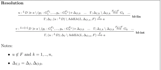
In the resolution system for LHHF proposed in [76], the authors first apply right rules to decompose and reduce non-atomic goal formulas. When the goal formula is finally atomic (a), a program formula (D) is selected from either the intuition-istic context or from the linear context. Resolution rules for selecting from the linear context and from the intuitionistic context are given in Figure 3.1.

D a \ G Γ, D; ∆I\ ∆O=⇒ G

Γ, D; ∆I\ ∆O=⇒ a res-atm int

D a \ G Γ; ∆I\ ∆O=⇒ G

Γ; ∆I, D \ ∆O =⇒ a res-atm lin

Figure 3.1: Resolution rules for the linear context and the intuitionistic context. In both cases, the program formula and the atomic goal are passed to a resid-uation judgment in order to produce a residual subgoal G to be subsequently proven. We should note that, if the program formula D is selected from the lin-ear context, then D is removed from the linlin-ear context to prevent reusing it. The residuation judgment takes the form

D a \ G ,

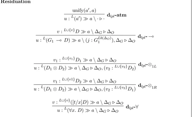
which stands to mean that the atomic goal a can be proven from the program D, assuming that a proof for the subgoal G can later be generated.

For example, the residuation rule for atomic resources is given as a0 a \ a0 _{= a}. dec-atm ,

where a and a0 are atomic formulas and we can have a solution if a and a0 are

equal.

The residuation rule for linear implication is given as

D a \ G0

(44)

where if we have the program formula G ( D, then we prove the atomic goal

a from the program formula D, while we add new subgoals G0 and G to the goal

context to prove all goals later.

3.2 The LPL Grammar and Sequent Definitions

In this section, we first introduce the LPL grammar, which is a similar version of the LHHF grammar. Afterwards, we introduce sequent definitions for LPL. We call this new resolution system BL.

3.2.1 The LPL Grammar

LPL is an extension of LHHF, with the addition of negative occurrences of simul-taneous conjunction (⊗). On the other hand, we exclude alternative conjunction (&), Top (>) and 1 from the LPL language, since we can still represent STRIPS style planning problems without these connectives. We implement these changes by first defining LPL through the grammar

Program formulas: D ::= a | D1⊗ D2 | G ( D | ∀x. D

Goal formulas: G ::= a | G1⊗ G2 | D ( G | D ⊃ G

| ∀x. G | a1

.

= a2 | !G | ∃x. G ,

where a denotes atomic formulas. The most important difference between the LHHF grammar and the LPL grammar is that we incorporate simultaneous con-junction (⊗) into program formulas. This addition lets us encode actions within task planning domain with formulas that can have multiple resources in their ef-fects for planning problems. In this grammar, we also exclude program formulas of the form G ⊃ D, since we can model this type of form through (!G) ( D. However, we need formulas of the form D ⊃ G in goal formulas since we do not allow negative occurrences of exponentials, !D.

(45)

3.2.2 Sequent Definitions of LPL

In order to present our backchaining resolution system for LPL, we now describe an associated sequent calculus formulation. Our sequent takes the form

Γ; ∆I\ ∆O F

=⇒ G , (3.1)

which enhances the system described in [76] with a number of improvements. This sequent definition captures the statement that the goal G can be proven using unrestricted resources from the multiset Γ and consumable resources from the

multiset ∆I, leaving resources in the output multiset ∆O unused. The forbidden

set, F , above the sequent arrow keeps a set of assumption labels from ∆I such

that no subproof of this sequent is allowed to use them in any way.

All program formulas in Γ and ∆ are assumed to be of the form (u : LD),

where u is an unique label assigned for each resource D. The presence of D in Γ or ∆ depends on a set of previously decomposed resources, with the superscript set L storing labels of these resources. We keep track of such dependencies to

control boundaries beyond which partially decomposed resources in ∆O should

not travel.

We now define our second judgment, residuation, motivated by [76] with a number of important improvements as

u :LD a \ ∆G. ∆O, (3.2)

where D is the program formula that we focus on (with dependency labels L),

and a is an atomic goal. ∆Gis a multiset of subgoal formulas, filled in by negative

occurrences of implication rules. Each resource in ∆G is the form of (ug : GF),

where ug is a unique subgoal label, G is the subgoal formula, and F is a list of

resource labels that should not be used in the proof of this subgoal. ∆O is a

multiset of sub-formulas of D that are left unused, filled in through simultaneous conjunction within D.

(46)

G in LPL if we can prove the sequent

·; · \ ·=⇒ G .∅

These enhancements of the language make it possible to incorporate negative occurrences of simultaneous conjunction (⊗), increasing the expressivity of LPL while preserving the complexity of the language compared to efficient languages such as LHHF. We should also note that unlike LHHF provers like Lolli, we are not particularly concerned with the uniformity of LPL proofs, since our goal is not the specification of a logic programming language. Instead of the uniformity, we are much more interested in the efficiency of proof search.

3.3 Proof Theory of LPL

In this section, we present a novel sequent calculus to perform proof search for BL , using the I/O model for resource management. This calculus, much like the

resolution calculus for LHHF (RM2), begins proof search by eagerly decomposing

the goal formula in the given sequent, using appropriate right rules (also called reduction rules). We categorize right sequent rules to two groups, multiplicative right rules in Section 3.3.1 and right rules for exponentials and quantifiers in Section 3.3.2. Once the goal formula is an atomic goal a, proof search continues by decomposing a program formula from either the unrestricted or the linear context, given in Section 3.3.3.

3.3.1 Multiplicative Right Rules

We already mentioned the meaning of each linear logic connective in Section 2.2.2. While describing proof rules for BL, we mostly focus on differences of BL

com-paring to RM2. We start with multiplicative right rules presented in Figure 3.2.

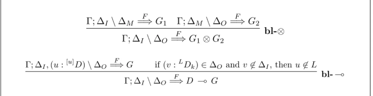
If the goal formula is composed with a simultaneous conjunction (⊗) or a linear implication ( ( ), we can apply multiplicative right rules.

(47)

Γ; ∆I\ ∆M F =⇒ G1 Γ; ∆M\ ∆O F =⇒ G2 Γ; ∆I\ ∆O F =⇒ G1⊗ G2 bl-⊗ Γ; ∆I, (u :[u]D) \ ∆O F =⇒ G if (v :LDk) ∈ ∆O and v 6∈ ∆I, then u 6∈ L Γ; ∆I\ ∆O F =⇒ D ( G bl- (

Figure 3.2: Multiplicative right sequent rules for the BL proof theory.

In the bl-⊗ rule, we decompose the goal and then achieve the first goal using

the input context ∆I, storing the leftover resources in ∆M. Subsequently, we

achieve the second goal using the leftover resources in ∆M.

Among multiplicative right rules for BL, the most interesting is perhaps the right rule for linear implication, bl- ( . Much like the standard right rule for this connective, we attempt to prove the subgoal G with the addition of new assump-tion D into the linear context. The primary difference is in the requirement that

none of the output resources in ∆O are allowed to depend on the newly

intro-duced resource D. This is necessary since, as we will see shortly, ∆O is no longer

a strict subset of the input context. Consequently, not only it is possible that the newly introduced resource ends up in the output context, but other resources that are derived from it by delayed application of left rules may also be left unused. Allowing those resources to cross this linear implication boundary would result in an unsound proof theory. The set of dependence labels, L, for resources in the output context will be maintained by resolution rules as we describe in the following sections.

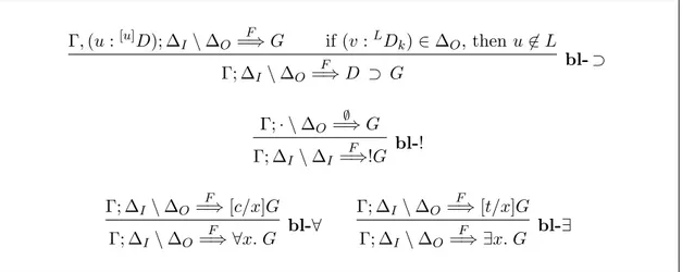
3.3.2 Right Rules for Exponentials and Quantifiers

In this section, we present four right rules for exponentials and quantifiers, given in Figure 3.3.

Linear planning logic and linear logic graph planner: domain independent task planners based on linear logic

LINEAR PLANNING LOGIC AND LINEAR

LOGIC GRAPH PLANNER: DOMAIN

INDEPENDENT TASK PLANNERS BASED

ON LINEAR LOGIC

a dissertation submitted to

the graduate school of engineering and science

of bilkent university

in partial fulfillment of the requirements for

the degree of

doctor of philosophy

in

computer engineering

By

Sıtar Kortik

September, 2017

ABSTRACT

LINEAR PLANNING LOGIC AND LINEAR LOGIC

GRAPH PLANNER: DOMAIN INDEPENDENT TASK

PLANNERS BASED ON LINEAR LOGIC

¨

OZET

DO ˘

GRUSAL PLANLAMA MANTI ˘

GI VE DO ˘

GRUSAL

MANTIK GRAF˙IK PLANLAYICI: DO ˘

GRUSAL

MANTIK TABANLI ALAN BA ˘

GIMSIZ G ¨

OREV

PLANLAYICILAR

Acknowledgement

Contents

List of Figures

List of Tables

Chapter 1

Introduction

1.1

Motivation and Scope

1.2

Contributions

1.2.1

Linear Planning Logic (LPL)

1.2.2

Linear Logic Graph Planner (LinGraph)

1.3

Organization of the Thesis

Chapter 2

Background and Related Work

2.1

Task (Action) Planning

2.2

Intuitionistic Linear Logic: Language and

Proof Theory

2.2.1

The Grammar and Connectives of Linear Logic

2.2.2

Sequent Calculus for Linear Logic

2.2.3

Proof Search in Linear Logic

Chapter 3

Linear Planning Logic: An

Efficient Language and Theorem

Prover for Robotic Task Planning

3.1

An

Overview

of

a

Resolution

System

for Linear Hereditary Harrop Formulas

(LHHF)

3.1.1

Resource Management

3.1.2

Backchaining and Residuation in LHHF

3.2

The LPL Grammar and Sequent Definitions