THE CHOICE OF INTEREST RATES IN PROJECT MANAGEMENT: THE CASE OF TIME VARYING INTEREST RATES
The Institute of Economics and Social Sciences Of
Bilkent University
By
Mustafa Kemal TOPCU
In Partial Fulfillment of the Requirements for the Degree of
MASTER OF BUSINESS ADMINISTRATION in
THE DEPARTMENT OF MANAGEMENT BILKENT UNIVERSITY
ANKARA September 2002
I certify that I have read this thesis and have found that it is fully adequate, in scope and in quality, as a thesis for the degree of Master of Business Administration.
--- Assist. Prof. Levent AKDENİZ
I certify that I have read this thesis and have found that it is fully adequate, in scope and in quality, as a thesis for the degree of Master of Business Administration.
---
Assist. Prof. Aslıhan SALİH-ALTAY
I certify that I have read this thesis and have found that it is fully adequate, in scope and in quality, as a thesis for the degree of Master of Business Administration.
--- Assist. Prof. Erdem BAŞCI
Approval of the Institute of Economics and Social Sciences
--- Prof. Kürşat AYDOĞAN Director
ABSTRACT
THE CHOICE OF INTEREST RATES IN PROJECT MANAGEMENT: THE CASE OF TIME VARYING INTEREST RATES
Topcu, Mustafa Kemal M.B.A., Department of Management Supervisor: Assist. Prof. Levent Akdeniz
September 2002
A study of existing and potential markets and of the technical and economical feasibility of a project, as well as sound finance planning, are indispensable.
Economic profitability is the obvious and most important criteria for industrial project evaluation.The choice of interest rates in project management is the purpose of the thesis.
The rate of interest should be adopted as discount rate in project evaluation. Because, the rate of interest reflects time preference and the opportunity cost of the possible alternative use of the capital invested. The interest rate is assumed to be constant during the project life in project evaluation techniques. In order to overcome this inability the constant rate should be replaced by time varying interest rates.
Several forecast models aid project management to predict the valid interest rates in the evaluation. The thesis employs the expected-change forecast model to obtain interest rates for each year during the life cycle. An application of the model to one of the large-scale projects in the Armed Forces, namely modern self-propelled direct support artillery gun- SP2000, is presented in the thesis. Comparison of two alternative uses of interest rates in the calculation of net present value of the project is discussed. It is concluded that the constant interest rate use overstates the costs and it is suggested that the time varying interest rates should be adopted as the optimal discount rates in project management.
ÖZET
PROJE YÖNETİMİNDE FAİZ ORANLARI SEÇİMİ:
DEĞİŞKEN FAİZ ORANLARININ KULLANILMASI DURUMUMustafa Kemal TOPCU
YÜKSEK LİSANS TEZİ, İŞLETME FAKÜLTESİ Tez Danışmanı: Yrd.Doç. Dr. Levent AKDENİZ
Eylül, 2002
Mevcut ve potansiyel piyasaların etüdü, projenin teknik ve ekonomik fizibilitesi finansal planlanlamayla beraber bir bütün halinde düşünülmelidir. Ekonomik karlılık endüstriyel proje değerlendirilmesi için en uygun ve en önemli kriterdir. Proje değerlendirilmesinde kullanılacak indirgeme oranlarının seçimi tezin konusudur.
Proje değerlendirmelerinde faiz oranı indirgeme oranı olarak kullanılmaktadır. Çünkü faiz oranı sermayenin zamansal tercihini ve olası alternatif kullanımların fırsat maliyetini yansıtır. Proje değerlendirmelerinde indirgeme oranı proje ömrü boyunca sabit kabul edilmektedır. Bu yetersizliği gidermek için değisken faiz oranları kullanılabilir.
Birçok tahmin yöntemi proje yönetimine değerlendirme esnasindaki faiz oranın tahmin etmede kolaylık sağlar. Tezde proje ömrü boyunca her yılki faiz oranlarinı elde etmek için beklenen-değişim tahmin modeli kullanılmıstır. Modelin Silahlı
Kuvvetlerdeki projelerden biri olan SP2000 projesine, kundağı motorlu direk destek topçusu silah sitemine, uygulanmasına yer verilmistir. Projenin net bugünkü
değerinin hesaplanmasinda kullanilan alternatif faiz oranlarinın karsılastırılması yapılmıstır. Sonuç olarak, sabit faiz oranlarının maliyeti olduğundan farkli gösterdiği elde edilmistir. Ve, proje yönetiminde değisken faiz oranlarının optimal indirgeme oranı olarak kullanılmalıdır.
ACKNOWLEDGEMENTS
I would like to thank to Assistant Professor Levent Akdeniz for his supervision, interest, and constructive comments throughout the thesis. I am also grateful to the examining committee members for their advice and suggestions.
TABLE OF CONTENTS
Abstract..……..………..iii
Özet……..………...v
Acknowledgements………...vii
Table of Contents……….. …...viii
List of Tables………….………..…….….ix
List of Figures……….………....x
CHAPTER 1: Introduction……….…1
CHAPTER 2: Literature Review………..……….4
CHAPTER 3: The Model……….………...………….………10
Data ………….……….12
Methodology ………..………..………12
Usefulness of the Model……….………..16
Result ……….………..17 CHAPTER 4: An Application…..……….……...19 Defense Industry ….……….……...19 SP2000 Project... ….………24 CHAPTER 5: Conclusion ……….……...28 BIBLIOGRAPHY ……….………...………31 APPENDICES…...……….………...…….……..33
Appendix-A Nominal Interest Rates for Dollar Denominated Deposits....33
Appendix-B Data for Forecast of Interest Rate as of January 2004.……..34
Appendix-C NPV For Varying Interest Rates……….……...35
LIST OF TABLES
Table-1. Coefficients of the Regression Model..………....15 Table-2. Summary Statistics for the Model………16 Table-3. Analysis of Variance for the Model…..………...17 Table-4. Economic and Military Data for Turkey and Neighbors…………..37 Table-5. Defense Industry Finance……….………38
LIST OF FIGURES
1. Normal P-P Plots of Residuals………...13 2. Probability Histogram of Residuals………....13
CHAPTER 1
INTRODUCTION
All developing countries suffer from shortage of capital, foreign exchange or skilled person; this calls for optimum utilization of available sources in order to achieve economic development. An industrial project should be evaluated in the context of the development needs of the economy. Industrial development takes into account both import substitution and export promotion.
A study of existing and potential markets and of the technical and economical feasibility of a project, as well as sound finance planning, are indispensable.
Economic profitability is the obvious and most important criteria for industrial project evaluation.
The purpose of the thesis is to determine an optimal discount rate for project management. The discount rate should be based on the actual rate of interest in the capital market to reflect the time preference and opportunity cost of the possible alternative use of the capital invested. The rate of interest is supposed to represent the time preference of public, expressing relative weights to be attached to present compared to future consumption. Secondly, it is supposed to express the productivity of private capital investment, and this represents the opportunity cost of public sector projects.
If the investment is financed by long-term loans, the actual rate of interest paid should be taken as the discount rate. If no loans are supplied for financing a project, the rate of interest charged by Central Bank should be adopted as the discount rate. To forecast the required interest rate, several forecast hypotheses, which are the error-learning model, return-to-normality model, expected-level model, and expected-change model, exist. The former two models are reduced forms of change model and the change model is also superior to expected-level model. Therefore, the expected-change model is employed in the thesis.
The aim of the Defense Industry Act is to develop a modern industry and establish stable conditions to provide modernization for Armed Forces. As a result of achievement of this goal, it is expected: to make use of present potential to maximum extent, to encourage and guide new high technological investments, to support research and development and to introduce new technologies, to accomplish a self-sufficient industry.
The interest rates forecasted by the model are applied to SP2000 Project: A direct fire support artillery main arm system production. NPVs for the project are calculated by using both a constant discount rate and time varying interest rates. The comparison is provided in the thesis.
The subject is studied in six chapters. The structure of the thesis follows: Chapter 2 provides literature review. The discount rate alternatives and the forecast models are discussed in the chapter.
Chapter 3 presents the forecast model in order to predict the time varying interest rates for the application of the prevailing interest rate as the discount rate in
project evaluation techniques. The forecast model is presented and the regression equation is obtained.
Chapter 4 presents a review of defense industry in Turkey and provides an application of the model to the project of an artillery weapon, a modern
self-propelled gun, SP2000, planned to be produced domestically. Analysis goes further with the discussion of the use of a constant interest rate and time varying interest rates.
Chapter 5 is the conclusion chapter including results, recommendations and the limitations of the thesis.
CHAPTER 2
LITERATURE REVIEW
In the project evaluation, several techniques can be used to figure out the cost of the project. Project evaluation techniques fall into two broad categories: those that consider the time value of money by discounting cash flows and those that do not.
Project evaluation techniques that ignore time value of money require some revenues in order to cover its investment. So that they are not available for nonprofit projects such as state projects, arms systems, and utility projects. It is recognized that net present value method is superior to the other methods. Stewart (1991) purports that one point worth noting is that the major drawback encountered when using the evaluation techniques is the choice of a discount rate. Project management should decide the basis of selecting the value of the discount rate from a number of choices. An incorrect discount rate could result in an incorrect investment decision.
Ayanoğlu, et al. (1996) claims that magnitude of discount rate affects project selection process and the results of analysis to a great extent as well as cash outflows and inflows. The error in calculation of the magnitude results in acceptance of a project, which would be rejected. Since the public sector projects are larger in magnitude, losses would be at the level that corruption would be costly or impossible.
Merrett and Sykes (1960) assume that firms anticipate their marginal cost of capital to be constant in the future at their current level. The marginal cost of capital is the discount rate that is the cost of the resources allocated for the project where the entrepreneur or the public gives up from consumption. That is to say, the discount rate figures the least rate of return on the project.
Dean (1968) mentions three alternative concepts of the cost of the capital of public projects. The fist concept is that capital is a free good. He cites three reasons for this belief. One is that government can create unlimited quantities of money. However, creating money does not increase real resources and this capital is paid for by instability and slow growth associated with inflation. Another reason is that government’s power to tax is unlimited. Capital obtained through increased taxation has a hidden cost in the form of a decaying growth rate, impaired investments and misallocation of resources. A third reason is that governments can get capital from more affluent nations in the form of gifts and loans that will never be paid. A second concept is that the cost of capital is the sum of the cost of capital to all the
corporations constituting the private enterprise sector of society in the nation concerned. A third concept is that the cost of capital is the government borrowing rate, which is visible market cost of borrowed capital.
Ayanoğlu, et al. discusses three ratios aid to figure out the discount rate: the interest rate paid for borrowed money, current interest rates in the capital markets (deposit rates, government bond rates), and rate of returns on similar projects. Lang and Merino (1993) implies that there is a strong consensus that project selection studies for governments should be based on returns at least equal to the cost of borrowing money. He also indicates that the rates of return for discounting cash
flows for public projects are generally lower than for private projects due to the absence of risk.
The discount rate should be based on the actual rate of interest in the capital market to reflect the time preference and opportunity cost of the possible alternative use of the capital invested. The rate of interest is supposed to represent the time preference of public, expressing relative weights to be attached to present compared to future consumption. Secondly, it is supposed to express the productivity of private capital investment, and this represents the opportunity cost of public sector projects.
Telser (1967) indicates that the current term structure forecasts the future term structure and expectations of future interest rates play an important role in the explanation of the term structure. But, forecasting interest rates is both a difficult and a valuable activity. Forecasters frequently use a time trend to aid their efforts because forecasting is a process of predicting the future values based on the knowledge of past performance.
Georgoff and Murdick (1991) summarized forecasting methods under four heads: judgment methods, counting methods, time series methods, and association or causal methods. Correlation methods, regression models, leading indicators,
econometric models, and input-output models are summarized as the association or causal methods. Regression models estimate the dependent variable via a predictive equation derived by minimizing the residual variance of one or more predictor variable. Forecasting regression models predict the future interest rates using a linear combination of past observations.
Kane (1969) posits that one can distinguish three broad forecasting
hypotheses: the error-learning model, the return-to-normality model, and the adaptive expectations model. Diller (1969) has shown that the first two models can each be regarded as a special case of the third.
Until the work of Meiselman (1962), comprehensive empirical testing of interest rate expectations was lacking. He developed an error-learning model and testing it with 1900-54 corporate-yield data, concluded that interest-rate expectations are revised according to the size of error between the forecast of the current rate given by the future rate and the current rate that subsequently appeared. He suggests that a forecast for a specific future rate would be revised as one moves closer to its date. Dobson, et al. (1976) repeated Meiselman’s study using corporate data and confirmed the findings that revision should be proportional to error made in forecasting present rate.
Meiselman correctly asserts that this model can say nothing about the level of expected interest rates but can only tell how expectations change. According to that hypothesis the market revises its expectations of all future short rates by a constant proportion of the error in the previous period’s forecast of the current short rate. Meiselman’s expected rates are the forward rates and are not weighted moving averages of past spot rates. Moreover, it has been shown by Telser that error-learning model is compatible with a set of different expectations about rates to prevail at different times in the future. On the other hand, Malkiel and Kane (1969) in particular tried to test the model by cross-section data and the study supports the hypothesis that error learning does occur, especially in predicting the course of short rates over short run. Albeit it has been shown that for longer rates and even for
shorter rates approximately fifteen months in the future, the evidence is much less convincing.
In return-to-normality models, interest rates are expected to return to a long-run normal level. As an alternative to Wood’s specification of long-long-run normal as a constant, long-run normal can be treated as a weighted average of past rates as suggested by Malkiel (1966). In his contribution to return-to-normality model Malkiel amended the model by assuming that the weights decline slowly and geometrically.
The adaptive expectations model was introduced by Cagan to measure price expectations in 1956. The model performed that task well and has since been used in a variety of applications. It has been suggested by Cagan that the error made in forecasting the current period will be used to adjust the old forecast to obtain the current expectation for the next period when the model is applied to the expectation of interest rates. Adaptive expectations model assumes that forecasts of future levels of the interest rate can be expressed as a distributed lag of the values observed for this rate in the past.
Diller has taken quite different approach to the problem of how expectations are formed by using first-order autoregressions. The results obtained by the study approves that spot rates may be forecasted at the basis of past spot rates by fitting autoregressions by least squares to the observed sequence of past spot rates. Diller attempts to explain forward rates in terms of past spot rates where the coefficients of past spot rates that were used to predict the revision of expectations. He also assesses the accuracy of forward rates as predictors of subsequent spot rates.
Kane introduces and tests an alternative method, which is expected-change model. This model concentrates on a structural model for forecasting cumulative changes in interest rates and presumes that level forecasts are derived as the sum of the current level and a forecasted cumulative change. Sinkey (1973) indicates that the expected change model is a structural model for forecasting not interest-rate levels, but cumulative changes in interest rates.
Kane’s model incorporates a linear distributed lag of previous interest-rate changes and a return-to-normality term. Sinkey shows the superiority of expected-change model over the expected-level model and concludes that the expected-change model is the better structural form compared to the forecasting hypotheses. He also purports the importance of expectational elements in determining the term structure of interest rates.
In Kane’s study comparison to former models are presented. The two models show the same intercept and goodness-of-fit. But, the two models place quite
different prior restrictions on the signs of coefficient estimates, cross-section and time series estimates are shown to conform rather closely to expected-change specification and to depart substantially from the requirements of the expected-level model.
CHAPTER 3
THE MODEL
The model used in the thesis depends on Kane’s expected-change model of interest rate forecasting. Kane’s own study shows that the model performs better on cross-section data. Sinkey tests the model against time series and the regression estimates strongly support the model.
The changes in interest rates are a combination of a lag of previous interest rate changes and a return-to-normality term. Basically the model assigns weights to changes expected or observed for the N periods preceding the forecast date. For the forecast span is greater or equal to three (k>= 3), the structure of the model is:
[
r r]
c[
r R]
c[
R t j]
u c a R r N k j j k t t t k t j k t t j k t k j j t t k t = + + ∑ − + − + ∑ ∆ − + − = + − + − − − + − − + + − = + 1( ) 0 1 1 1 1 2 1 2 1 1 3 0 1A lowercase r stands for a forecast value and an uppercase R for an interest rate observed in the market. Pre-subscripts indicate the date at which a rate applies or is expected to apply, the post-subscripts are the maturity period, the date that market rate is observed or forecast is made, and the application date of forecast, respectively. And u is the stochastic term that is assumed to be normal with a mean of zero and a variance equal toσ . It is also assumed that the random errors be independent. 2
When forecast span equals to two (k=2), the first sum drops out and equation becomes:
[
r R]
c[
R t j]
u c a R r N k j k j t t t k t t k t = + + − +∑
∆ − + − = + − + − + 1( ) 0 1 1 1 1 2 1When forecast span is decreased to one (k=1), the notation between sums also drops out and then the equation becomes:
[
R t j]
u c a R r N k j k j t t k t = + +∑
∆ − + − = + − + 1( ) 0 1 1In the thesis the forecast span is assumed to be equal to twelve so that the first equation is used and rearranged as:
[
]
[
]
12[
1( )]
0 11 1 1 1 10 1 10 11 9 0 1 12r R a c r r c r R c R t j j j t t t t j t t j t j j t t t − = +∑
− + − +∑
∆ − = + + − + − + = +Equation is a general expression, which incorporates the hypothesis that the structure of interest rates is primarily determined by expectations of the future course interest rates and that these expectations in turn are generated by a distributed lag on past rates. The left hand side of the equation asserts yearly change of the interest rate. This is the difference between the forecasted value of twelve-month ahead and the observed market rate when the forecast is made. Since the monthly interest rates are used in the thesis, forecast span is assumed to be equal to twelve for finding the interest rate that will apply to one year later. a is the constant coefficient of the regression model and expected to be zero. The right hand side of the equation is the presentation of the lags of twenty-four preceding months. Since the actual values are
not known between t+1 and t+k-1, the forecasted values are used instead of the actual values.
Data
The period for data is between March 1990 and June 2002. Monthly nominal interest rates with the maturity of one year are presented in Appendix-A. The rates of interests are the yearly-observed market rates in a monthly interval. Thus, it is aimed to smooth the fluctuation during the year and to use more recent data.
If no loans are supplied for financing a project, the rate of interest charged by Central Bank should be adopted as the discount rate. Since projects are largely dollar oriented, interest rates used in the model are dollar denominated deposit rates
reported by the Central Bank of Turkey. Data are available on the World Wide Web page of the Central Bank.
Methodology
SPSS 10.0 for Windows Statistical Software Package is employed in the thesis. Linear regression model is used to relate the time series of interest rates and the least squares method is used to forecast future values of interest rates. The notion of fitting a curve to a set of sufficient points is essentially the problem of finding the parameters of the curve. Since the desired equation is to be used for predicting the future interest rates, it is useful to require that the equation be so modeled as to make the errors of prediction so small. Thus, the least squares method is used. An error of the prediction means the difference between an observed value and the
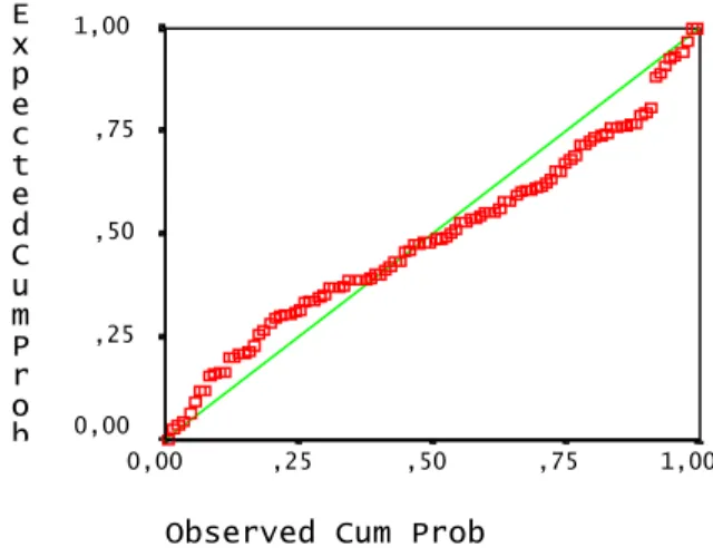
residuals and Figure 6 is the histogram presentation of the probabilities. The
variation of the residuals is,σ = 2,939*102 -5 and the standard error of the estimate is
5,42*10 -3. The magnitude of the standard error of the estimate is the indicator of the acceptance of the least squares method. And the expected changes will take place within two standard error. It is expected to fall within the interval of 1,08* 10 2.
Observed Cum Prob
1,00 ,75 ,50 ,25 0,00 E x p e c t e d C u m P r o b 1,00 ,75 ,50 ,25 0,00
Figure 1 Normal P-P Plots of Residuals
Regression Standardized Residual
4 3 2 1 0 -1 -2 -3 30 20 10 0 Std. Dev = ,94 Mean = 0,00 N = 106,00 -4 F r e q u e n c y
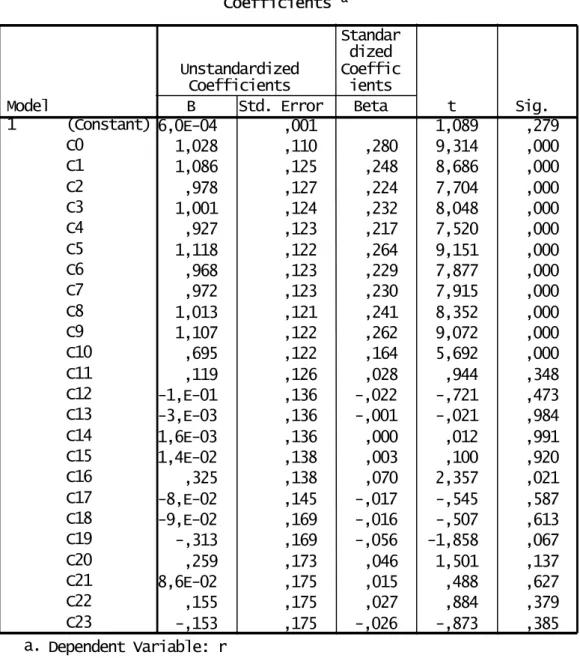
Sample size is 106. Sample is large enough to make inferences about the forecast model. Table- 1 is the coefficients of the model with t-statistics and
observed significance levels. The constant coefficient is zero as expected. The other coefficients are expected to be one. The first eleven lags’ coefficients are
significantly different from zero and around one as expected. The rest seems insignificant. This is a signal that the independent variables may contribute
redundant information. The interdependent variables could be correlated with each other. The first eleven lags contribute more information for predicting the interest rate, but the other lags still alone contributes information for the prediction. In the time-series model general problem is the correlated data.
The Durbin-Watson statistic (d) is used to test for the presence of first-order autocorrelation. The correlation between time series residuals at different points in time is called autocorrelation. Correlation between neighboring residuals (at times t and t+1) is called first-order autocorrelation. The value of d always falls in the interval from 0 to 4. If the residuals are uncorrelated then d is approximately 2. If the residuals are positively correlated, then d is greater than 2, if the relation is very strong then d is exactly 4. If the residuals are negatively correlated then d is less than two, if the correlation is very strong then d is absolutely 0. The model
Durbin-Watson statistic is 2,014, indicating that the residuals are not correlated. Therefore, the model provides sufficient information for the prediction of the interest rates.
Table 1 Coefficients for the Regression Model Coefficients a 6,0E-04 ,001 1,089 ,279 1,028 ,110 ,280 9,314 ,000 1,086 ,125 ,248 8,686 ,000 ,978 ,127 ,224 7,704 ,000 1,001 ,124 ,232 8,048 ,000 ,927 ,123 ,217 7,520 ,000 1,118 ,122 ,264 9,151 ,000 ,968 ,123 ,229 7,877 ,000 ,972 ,123 ,230 7,915 ,000 1,013 ,121 ,241 8,352 ,000 1,107 ,122 ,262 9,072 ,000 ,695 ,122 ,164 5,692 ,000 ,119 ,126 ,028 ,944 ,348 -1,E-01 ,136 -,022 -,721 ,473 -3,E-03 ,136 -,001 -,021 ,984 1,6E-03 ,136 ,000 ,012 ,991 1,4E-02 ,138 ,003 ,100 ,920 ,325 ,138 ,070 2,357 ,021 -8,E-02 ,145 -,017 -,545 ,587 -9,E-02 ,169 -,016 -,507 ,613 -,313 ,169 -,056 -1,858 ,067 ,259 ,173 ,046 1,501 ,137 8,6E-02 ,175 ,015 ,488 ,627 ,155 ,175 ,027 ,884 ,379 -,153 ,175 -,026 -,873 ,385 (Constant) C0 C1 C2 C3 C4 C5 C6 C7 C8 C9 C10 C11 C12 C13 C14 C15 C16 C17 C18 C19 C20 C21 C22 C23 Model 1 B Std. Error Unstandardized Coefficients Beta Standar dized Coeffic ients t Sig. Dependent Variable: r a.
Usefulness of the Model
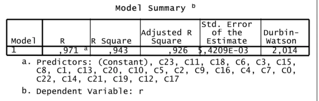
Goodness-of-fit is measured by the coefficient of determination or standard error of estimate. Multiple Coefficient of Determination (R2) represents the fraction of sample variation of the regrassand value that is explained by least squares
prediction equation. R2 is a sample statistics that tells how the model fits data.
Table 2 Summary Statistics for the Model
Model Summary b
,971 a ,943 ,926 5,4209E-03 2,014
Model 1
R R Square Adjusted RSquare
Std. Error of the
Estimate Durbin-Watson Predictors: (Constant), C23, C11, C18, C6, C3, C15, C8, C1, C13, C20, C10, C5, C2, C9, C16, C4, C7, C0, C22, C14, C21, C19, C12, C17 a. Dependent Variable: r b.
About 94,3% of the sample variation in interest rates can be explained by using distributed lags to predict the interest rate in the regression model. It means that 94,3% of the variation in interest rate forecast for this sample is accounted by the model. To test the significance of accuracy, the hypotheses can be written as:
0 ... 2 1 0 =c =c = =ck = H = A
H At least one of the coefficients is nonzero
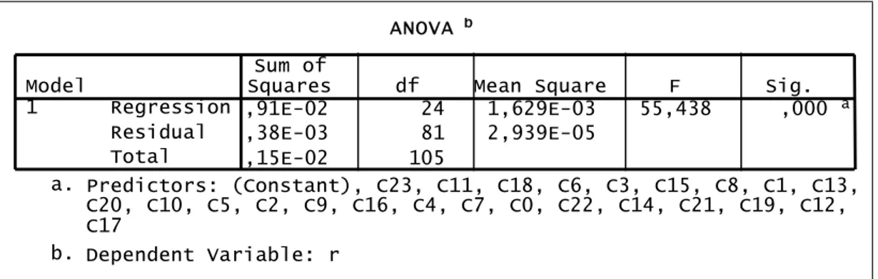
The statistic F has the F distribution with 24 and 81 degrees of freedom and may be used to test the null hypothesis that the coefficients of the model contribute no information. The F statistics has an observed significance level of 0,000 so that the null hypothesis is rejected. It appears that at least one of the coefficients differs
from zero. It is concluded that the model contributes information for predicting the future interest rates.
Table 3 Analysis of Variance for the Model
ANOVA b 3,91E-02 24 1,629E-03 55,438 ,000 a 2,38E-03 81 2,939E-05 4,15E-02 105 Regression Residual Total Model 1 Sum of
Squares df Mean Square F Sig.
Predictors: (Constant), C23, C11, C18, C6, C3, C15, C8, C1, C13, C20, C10, C5, C2, C9, C16, C4, C7, C0, C22, C14, C21, C19, C12, C17 a. Dependent Variable: r b. Result
The regression equation with the coefficients can be written as:
) 12 ( 1 ) 11 ( 1 ) 10 ( 1 ) 9 ( 1 ) 8 ( 1 ) 7 ( 1 ) 6 ( 1 ) 5 ( 1 ) 4 ( 1 ) 3 ( 1 ) 2 ( 1 ) 1 ( 1 1 1 1 1 1 1 1 2 1 2 1 3 1 3 1 4 1 4 1 5 1 5 1 6 1 6 1 7 1 7 1 8 1 8 1 9 1 9 1 10 1 10 1 11 1 1 12 153 , 0 155 , 0 086 , 0 259 , 0 313 , 0 09 , 0 08 , 0 325 , 0 014 , 0 0016 , 0 003 , 0 100 , 0 119 , 0 ) ( 695 , 0 ) ( 107 , 1 ) ( 013 , 1 ) ( 972 , 0 ) ( 968 , 0 ) ( 118 , 1 ) ( 927 , 0 ) ( 001 , 1 ) ( 978 , 0 ) ( 086 , 1 ) ( 028 , 1 − − − − − − − − − − − − + + + + + + + + + + + + + + + + + + + + + + ∆ − ∆ + ∆ + ∆ + ∆ − ∆ − ∆ − ∆ + ∆ + ∆ + ∆ − ∆ − ∆ + − + − + − + − + − + − + − + − + − + − + − + = t t t t t t t t t t t t t t t t t t t t t t t t t t t t t t t t t t t t t t t t t t t t t t t t t t t t t t t t t t t t R R R R R R R R R R R R R R r r r r r r r r r r r r r r r r r r r r r R r t
t+12r1 is the regressand that is the interest rate one year later from the date of
forecast. tR1 is the observed market rate when the forecast is done. t+11r1t−t+10r1t, …,
t t t
t+1r1 − R1 are the differences between subsequent two months forming first eleven
Should the resulting estimated equation explain the data satisfactorily, it can be concluded that the expected-change hypothesis is consistent with the observation of deposit rates. It is possible to conclude that the expectations hypothesis is
CHAPTER 4
AN APPLICATION
This chapter provides an application of the model to a defense industry project
.
Initially a brief review of the defense industry structure and finance method is necessarily presented and then the project definition and the application are provided.DEFENSE INDUSTRY
Defense industry is a sector aiming to produce very special products, namely arms systems, for a particular market, i.e. the customer is the States, within
distinctive environment. Defense Industry Policy and Strategy Application Directive of Ministry of National Defense present an official definition of the defense industry as the institutions that produce war weapons, vehicle, equipment, substitutes, and significant inputs with related products and services of those.
Since the output of the system is national security protection of the country, defense industry has different attributes relative to other industries. As a
monopsonist, the government not only sets the product specifications, but also the level of demand for the products. A continuous production that conform high quality specifications requires large investments and research and development studies.
Defense industry products operate under heavy meteorological and
oceanographical conditions. Also, costs increase relative to years and development of a new system takes seven to ten years while implementation takes three to five years. Another important feature is being regulated and financed by the Government.
Turkey’s geopolitical position is the dominant factor influencing Turkish military aims. At the convergence of Caucasus, Middle East, and the Balkans, and surrounded by seas and situated in the most sensitive and tentative region in the world, Turkey needs to improve army, navy, and air force altogether comparatively to many countries.
Aeronautics, artillery and ammunition production in Turkey along with maintenance and overhaul facilities were established during the early years of the Republic. However, in 1950s increase in military equipment assistance as a result of involving in NATO slowed down the defense industry in its early stages and raised dependence on foreign military equipment.
The U.S sanctions on arms deliveries to Turkey during and after Cyprus Operation made it clear that foreign dependence jeopardize the secure access to arms and domestic defense industry would be established immediately. The main goal of defense industry was import substitution, relieving of dependency to foreign military equipment. Turkey aimed to develop a modern arms industry, which would rather have export target.
The political and economical instability of the late 1970s decreased the pace of development. Between 1980 and 1983 the armed forces prepared a comprehensive modernization plan. In 1985 by the Act No. 3238, defense industry structure was
organized. Thus, it is foreseen that Turkey establishes its own defense technology and integrates the private sector into the industry in the long-run. The new system brings out a new infrastructure for defense decision making to plan, finance, implement, and supervise its fulfillment.
The new system brings out five main committees and foundations in order to plan, finance, implement and supervise its fulfillment. These are DISBC (Defense Industry Supreme Board of Co-ordination), DIEC (Defense Industry Executive Committee), UDI (Undersecretariat for Defense Industries), DISF (Defense Industry support Fund), and Audit Board in order of decision and implementation.
Defense industry requires quite high financial resources. Industrial investments are made in large quantities and generally financed by Government Budget. Industry also makes use of the resources that should be utilized for economic growth and improvement of social welfare. Especially in the less developed
countries, due not to have a qualified domestic industry, governments transfer all available resources to procurement of arms systems. This will probably result in a decrease in the welfare. On the other hand, defense industry has positive causations through the economy.
Hardly possible for developing countries is to invent and invest in the R&D. However, these countries may contribute to the production with rational allocation and productive use of resources. As Todd (1990) points out that all
advanced-industry country governments have urged their military-advanced-industry enterprises to chase after export opportunities in order to boost the economy.
Günlük-Şenesen (1993) summarizes the officially expected spill-over expects of a modern arms industry as more diverse industrial production, efficiency in
production, product quality improvement, foreign exchange savings, acceleration of economic growth, increased value added, decreasing unemployment, increases in the overall technology level, and improvement in the quality of the labor force and university education.
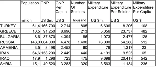
In a period of falling investment in the military sector in the world and
NATO, Turkey emerges as an exception. There is a shrink in the military expenditure overall in the world. Table 4 shows a comparison of economic and military data for Turkey and neighbors.
Table 4 Economic and Military Data for Turkey and Neighbors
Population million GNP US $m. GNP Per Capita US $ Number Of Soldiers Thousand Military Expenditure US $m. Military Expenditure Per Soldier US $ Military Expenditure Per Capita US $ TURKEY 61,4 166.700 2.714 805 6.606 8.206 108 GREECE 10,5 91.250 8.696 213 5.056 23.737 482 BULGARIA 8,6 37.670 4.394 86 1.073 12.477 125 RUSSIA 148,3 664.000 4.478 1.400 76.000 54.286 512 ARMENIA 3,5 8.498 2.453 60 79 1.317 23 IRAN 64,6 158.200 2.449 440 4.191 9.525 65 IRAQ 17,9 1.296 723 475 9.698 20.417 542 SYRIA 15,1 49.520 3.283 320 3.563 11.134 236 Source: Tübitak, 1998
Although Turkey has built up arms industry, it is still mainly dependent on arms imports and takes the third position in the major recipients during the period 1994-1998. Establishing an import substitution national defense industry requires large investments. Therefore, like other developing countries, Turkey allocates most resources in military expenditure. As of 1995, Turkey, having a 61 million
population, has $166.7 million GNP and makes $108 of military expenditure per capita. In 1999, Turkey experience expenditure per capita of $156, with a $193,5 million GNP and military expenditure occur with a change of $1,2 billion.
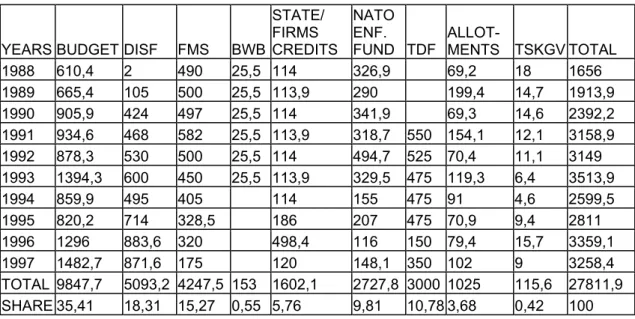
Finance of these expenditures is met highly by government budgets for many countries. This is due to feature of defense being exactly public product. In Turkey funds for defense finance are government budget, USA and Germany defense aids (BWB), equipment transfers as a result of discounts on sales in accordance with South Wing Act and AKKA Treaty, Defense Industry Support Fund (DISF), Turkish Defense Fund (TDF) established by U.S.A., Turkey, Saudi Arabia, Kuwait, and U.A.E, Turkish Armed Forces Foundation (TSKGV), and other aids provided by treaties.
Resources from government budget form the highest proportion for finance, %36 of total finance sources. Yet there is a decrease trend. The main factors are U.S.A and NATO aids and later establishment of funds, like TSKGV and DISF.
Table 5 Defense Industry Finance (US $m.)
YEARS BUDGET DISF FMS BWB
STATE/ FIRMS CREDITS
NATO ENF.
FUND TDF ALLOT-MENTS TSKGV TOTAL 1988 610,4 2 490 25,5 114 326,9 69,2 18 1656 1989 665,4 105 500 25,5 113,9 290 199,4 14,7 1913,9 1990 905,9 424 497 25,5 114 341,9 69,3 14,6 2392,2 1991 934,6 468 582 25,5 113,9 318,7 550 154,1 12,1 3158,9 1992 878,3 530 500 25,5 114 494,7 525 70,4 11,1 3149 1993 1394,3 600 450 25,5 113,9 329,5 475 119,3 6,4 3513,9 1994 859,9 495 405 114 155 475 91 4,6 2599,5 1995 820,2 714 328,5 186 207 475 70,9 9,4 2811 1996 1296 883,6 320 498,4 116 150 79,4 15,7 3359,1 1997 1482,7 871,6 175 120 148,1 350 102 9 3258,4 TOTAL 9847,7 5093,2 4247,5 153 1602,1 2727,8 3000 1025 115,6 27811,9 SHARE 35,41 18,31 15,27 0,55 5,76 9,81 10,78 3,68 0,42 100 Source: Defense and Aerospace
SP2000 PROJECT
There is an emphasis on total project cost, to include the entire stream of cost consequences over the life of a project. Research and development, production, operation and maintenance, support and disposal, which highlight the major phases in the life cycle, are the cost categories. Thus, life cycle cost method is mostly and widely used method in the military cost analysis. The life cycle cost is the sum of all costs, namely total procurement and ownership costs, incurred during the life of the project. Kinch (1993) states that there are three main reasons of using life cycle cost method in defense industry. Initially, the acquisition cost of the arms systems is too high. Next, defense industry projects have longer economic life. And the third is the occupation of operation and maintenance costs higher proportion in the total cost.
In order to provide immediate fire support with high accuracy to combat units, artillery weapon systems’ modernization requirement is one of large-scale projects in Turkish Army. It is aimed to produce a modern self-propelled gun, named SP2000, to provide continuous fire support, to change position quickly, and to meet the maintenance needs mostly by the first-level users. The research and development phase is successfully completed and the gun is practiced in the field exercises. Entirely financed by national resources, the direct support artillery main arms system modernization will be completed by production of SP2000.
The cost analysis of main artillery weapon system of Turkish Army, SP2000, is done according to life cycle cost method. Economic life of the project is assumed to be thirty years. Disposal cost of the project is assumed to be zero. Because of the
high change of the technology in defense industry, products after completion of the economic life have no opportunity to be sold. The products are generally exported as a military aid to allied countries. Thus, disposal cost is out of consideration. Grosse and Proschan (1965) point out that military projects also exclude the sunk costs as a decision-making relative to project choices and only include the net resource
requirements’ costs.
Research and development phase was completed within two years. In the second year the practices were executed and successful results were obtained. As the completion of research and development, production was initiated. Operation and maintenance costs form the higher proportion of the yearly costs. Operation costs comprise personnel salaries, ammunition costs, fuel consumption, and equipment costs. Maintenance costs stem from maintenance personnel salaries, lubrication and periodic control costs, and reserve for part changes.
Project evaluation techniques consider both costs and benefits. However, military arms system projects should be evaluated by their costs. Consideration on costs is not only focused on total project cost but also on the timing of the costs. This mentions the discounting problem and the importance of budgetary constraints. Thus, net present value method is the appropriate technique for defense projects. Military project cost analysis tends to be largely dollar-oriented. By using the discount rate future costs are discounted to present values. The discount rate should not be increased to accommodate expected uncertainties in the cost of capital since the values of the cash flows over time could not be realistically interpreted.
For economic life of the project, periodic costs are discounted to the present values. In defense industry the discount rate is assumed to be about 3% or it is taken as the credit rate, 4%, offered by the foreign countries that sell the arms system and offer the credit for payment. In the current application of project evaluation depends on the assumption that the discount rate is constant during the project.
The regression model found in the former chapter in this thesis provides the interest rates that are used to discount future costs to the present. Project start date is assumed to be January 2004 and the time varying interest rates are calculated by the regression equation. Data for forecast of interest rates as of January 2004 is provided in Appendix-B. Since the model incorporate the distributed lags and assign the weights, the changes between subsequent periods is also presented adjacent to interest rates.
By using data the forecast value for interest rate as of January 2004 is 4.31%. Available data at hand are for the period till June 2002. Thereafter, the regression model forecasts data for the period between June 2002 and December 2003 are used in order to forecast the interest rate valid for the project start date. Since the rates for the period between k+1 and k+11 are not known, the forecasted values are
substituted for unknown actual values.
In a similar trend, the interest rate for each year is figured out by the regression equation. The annual future cost of the project is discounted by the interest rate for the referred year in order to obtain net present value of annual cash flows. For example, discounting of the fifth year’s cash flow is straightforward. At
first, the cash flow is discounted by the interest rate for fourth year. Similarly, procedure goes on discounting the cash flow by the preceding year’s interest rate. Finally the net present value of the fifth year’s cash flow is retrieved on the project start date. One point is worth noting that cost estimates show the allotment from the budget for the project. Allotments start being used in the beginning of each year. So that each year’s cash flows are discounted by interest rate of the preceding year. Applying the likewise methodology, net present value of the project for time varying interest rates can easily be figured out. Appendix-C includes the excel sheet
calculation of net present value of each year and total net present value of the project via time varying interest rates.
Appendix-D presents the components of the cost, the cash flows for each year, and the discounted cash flows for a constant rate of 3%. The project cost according to constant interest rate is $3.555.039,80. As expected, the project cost for time varying interest rates differs and net present value of the project is
$3.070.976,61. The use of a constant interest rate does not reflect time preference and the opportunity cost of the capital invested. This will lead to distort in the cost frame and incorrect decision in project management. On the other hand, time varying interest rates sufficiently reflect the time preference, expressing relative weights to be attached to present compared to future cash flows.
CHAPTER 6
CONCLUSION
Major drawback encountered when using project evaluation techniques is the choice of discount factor. In the thesis, it is aimed to choose an optimal discount rate which fully reflect time preference and the opportunity cost of capital and the
application of the obtained time varying interest rates as the discount rates to SP2000, the direct fire support artillery main arms system project, is presented.
The monthly interest rates of dollar denominated deposits with a maturity of one year reported by the Central Bank of Turkey was used in the thesis to obtain the interest rates which would be used as discount rate in the projects. By applying the expected-change forecast model to data, regression equation was formed by the least squares method. For the beginning date of the project, January 2004, the interest rate was forecasted as 4,31%. And as a further step, the interest rates for each year during the project life cycle were predicted.
The discount rate in project evaluation is assumed to be constant. The
discount rate is either roughly an estimate of current market interest rate or the credit rate offered by supplier. However, the rates of interest are supposed to change year by year. Net present values of alternative discount rates are provided for the cost
analysis of the project. Net present value of the project by using time varying interest rates forecasted by the expected-change model is $484.063,19 less than that of the constant interest rate. NPV of the project for a constant rate is $3.555.039,80 and that for time varying interest rates is $3.070.976,61. The overstated costs by the choice of lower rates require the allocation of resources higher than needed. Moreover, the choice of lower discount rate make the resources idle and the opportunities would be forgone. The lower the rate of discount is chosen, the less future consumption will be discounted in relation to present, and the higher savings is needed.
It is possible to conclude that the magnitude of discount rate affects project selection process and the results of analysis as well as net cash flows. An incorrect discount rate could lead to an incorrect investment decision. The error in calculation of the magnitude results in acceptance of a project, which would be rejected. Since the defense industry projects are larger in magnitude, losses incurred by selection an incorrect project would be at the level that corruption would be costly or impossible.
It is suggested by thesis that time varying interest rate should be adopted as discount rate in order to reflect time preference and opportunity cost of the capital invested. The interest rates are supposed to change due to macroeconomic factors. Thus, the revision of the forecast model in further years will lessen the probable errors in the prediction of interest rates.
The thesis provides cost comparison of two alternative use of discount rate in project management, constant versus time varying. However, cost of the project is determined by fixed exchange rate. As an extension of the study, exchange rates can be forecasted and applied in the project management.
There are some limitations in the thesis. In the calculation of net present values, the thesis used nominal interest rates for dollar denominated deposits because military acquisitions and productions largely are dollar oriented. Since the inflation rate as dollar denominated is not available, it is appropriate to use the nominal rates. It is obvious that long-run interest rates are not the same with short- term rates. Although in the short run there exists changes in the rates, interest rates are assumed to be constant during the life of the project.
There is also a problem of divergence between the market price of capital and its social cost in developing countries. In perfectly competitive markets, the rate of interest represents the time preference and expresses the productivity of productivity of capital. In developing countries this discrepancy occurs because the rate of interest doe not correspond to both magnitudes.
Finally, the thesis provides the application with hypothetical data imputed by a recent study via life cycle cost method. Because of confidentiality and security actual data is not presented. Defense industry needs to be evaluated as a political and strategical venture as well as military and economical.
BIBLIOGRAPHY
Ayanoğlu, Kamil, İlter, Niyazi, Düzyol, M. Cüneyd, Yılmaz, Cevdet. 1996. Kamu Yatırım Projelerinin Planlanması ve Analizi.(State Investment Projects Planning and Analysis). Anakara:DPT.
Cagan, Philip. 1956. “The Monetary Dynamics of Hyperinflation.” In Friedman, Milton, ed., Studies in the Quantity of Theory of Money. Chicago: University of Chicago Press.
Dean, Joel. 1968.“Financial Planning of Industrial Projects and Their Appraisal.” In
Evaluation of Industrial Projects, Project Formulation and Evaluation Series, Vol. I.
New York: UN.
Diller, Stanley. 1969. “Expectations in the term structure of interest rates.” In Mincer, Jacob, ed., Economic Forecasts and Expectations. New York: Columbia University Press for the National Bureau of Economic Research.
Dobson, Steven W., Sutch, Richard C., and Vanderford, David E. 1976. “An
evaluation of alternative empirical models of the term structure of interest rates,” The
Journal of Finance 31(4): 1035-1065.
Georgoff, David M. and Murdick, Robert G. 1991. “Manager’s Guide to Forecasting.” In Accurate Business Forecasting, A Harvard Business Review Paperback. U.S.A: HBR Press.
Grosse, Robert N., and Proschan, Arnold. 1965. “Military Cost Analysis,” The
American Economic Review 55 (1/2): 427-433.
Günlük-Şenesen, Gülay. 1993. “An overview of the arms industry modernization programme in Turkey.” In SIPRI Yearbook 1993 World Armaments and
Disarmaments. New York: Oxford University Press.
Kane, Edward J. 1969. “The Term Structure of Interest rates: An Attempt to Reconcile Teaching with Practice,” The Journal of Finance 25(2): Papers and Proceedings of the Twenty-Eighth Annual Meeting of the American Finance Association New York, N.Y.: 361-374
Kinch, M.J. 1993. “Life Cycling Costing in The Defense Industry.” In Bull, J.W, ed.
Life Cycle Costing for Construction. London: Blackie Academic&Professional.
Küçüktepe, Olcay. 2000. Comparison of Two Artillery weapon System by Using Life Cycle Cost Technique. Ankara: Bilkent University
Lang, Hans J., and Merino, Donald J. 1993. The Selection Process for Capital Projects. New York: John Wiley&Sons Inc.
Malkiel, Burton G.1966. The Term Structure of ınterest Rates: Expectations and Behavior Patterns. New Jersey: Princeton University Press.
Malkiel, Burton G., and Kane, Edward J. 1969.“Expectations and Interest Rates: A Cross Sectional Test of the Error-Learning Hypothesis,” The Journal of Political
Economy 77 (4) part1:453-470
Meiselman, D. 1962. The Term Structure of Interest Rates. New Jersey:Englewood Cliffs.
Merrett, Anthony, and Sykes, Allen. 1960. “Calculating the Rate of Return on Capital Projects,” Journal of Industrial Economics 9(1): 98-115
MSY:317-3 Turksh Defense Industry Policy and Strategy Application Directive. Ankara: Ministry of National Defense.
Sinkey, Joseph F.Jr. 1973. “The Term Structure of Interest Rates: A Time-Series Test of the Kane Expected-Change Model of Interest Rate Forecasting,” Journal of
Money, Credit, and Banking 5(1) part 1: 192-200
Stewart, Rodnay D. 1991. Cost Estimating (2nd. Ed.). U.S.A: John Wiley&Sons Inc. Telser, L.G. 1967. “A Critique of Some Recent Empirical Research on the
Explanation of the Term Structure of Interest Rates,” The Journal of Political
Economy 75 (4) part 2: Issues in Monetary Research, 1966: 546-561
Todd, Daniel. 1988. Defense Industries: A Global Perspective. New York: Routledge Tübitak, 1998
Wood, John H. 1964. “The Expectations Hypothesis, the Yield Curve, and Monetary Policy,”Quarterly Journal of Economics 78: 457-470.
APPENDIX – A
Nominal Interest Rates for Dollar Denominated Deposits (%)
Source: Central Bank of Turkey
MONTH YEARS 1990 1991 1992 1993 1994 1995 1996 1997 1998 1999 2000 2001 2002 JANUARY N/A 9,20 5,90 4,20 4,50 5,10 6,50 7,30 9,30 11,50 10,90 13,20 4,50 FEBRUARY N/A 9,50 5,80 4,20 4,50 5,40 7,10 6,90 9,30 11,80 10,50 13,60 4,40 MARCH 7,70 9,60 5,40 4,20 4,90 5,60 7,20 7,10 9,70 11,90 10,70 12,90 4,40 APRIL 7,90 9,50 4,80 4,40 5,10 5,60 7,70 7,10 9,70 11,00 10,20 14,00 4,50 MAY 7,90 9,70 4,80 4,60 5,30 5,60 7,70 7,30 9,70 11,40 10,40 11,70 4,40 JUNE 8,00 9,50 4,70 4,40 5,80 6,00 7,70 7,60 9,80 12,00 10,30 11,20 4,50 JULY 8,10 9,00 4,50 4,30 5,50 6,70 6,80 7,90 10,20 14,40 10,20 11,20 N/A AUGUST 8,10 8,80 4,40 4,20 5,20 6,80 6,80 8,50 10,40 14,10 9,90 9,60 N/A SEPTEMBER 8,50 8,50 4,20 4,00 4,90 6,60 7,50 9,00 10,50 14,10 10,50 7,40 N/A OCTOBER 8,50 7,90 4,20 4,00 4,80 6,80 7,30 9,40 10,50 12,80 10,80 6,20 N/A NOVEMBER 8,60 7,00 4,20 4,10 4,80 6,20 7,60 9,40 10,90 12,50 10,90 5,10 N/A DECEMBER 9,00 6,30 4,20 4,50 5,90 6,50 8,00 9,30 10,90 12,30 14,00 4,80 N/A
APPENDIX- B
Data for Forecast of Interest Rate as of January 2004
1999 2000 2001 2002 2003 MONTH tR1 t+1r1t -tr1 tR1 t+1r1t -tr1 tR1 t+1r1t -tr1 tR1 t+1r1t -tr1 tR1 t+1r1t -tr1 JANUARY 11,50% 0,006 10,90% -0,014 13,20% -0,008 4,50% -0,003 6,02% 0,008 FEBRUARY 11,80% 0,003 10,50% -0,004 13,60% 0,004 4,40% -0,001 4,68% -0,013 MARCH 11,90% 0,001 10,70% 0,002 12,90% -0,007 4,40% 0,000 4,78% 0,001 APRIL 11,00% -0,009 10,20% -0,005 14,00% 0,011 4,50% 0,001 4,43% -0,004 MAY 11,40% 0,004 10,40% 0,002 11,70% -0,023 4,40% -0,001 5,19% 0,008 JUNE 12,00% 0,006 10,30% -0,001 11,20% -0,005 4,50% 0,001 4,68% -0,005 JULY 14,40% 0,024 10,20% -0,001 11,20% 0 4,77% 0,003 4,91% 0,002 AUGUST 14,10% -0,003 9,90% -0,003 9,60% -0,016 4,18% -0,006 3,73% -0,012 SEPTEMBER 14,10% 0 10,50% 0,006 7,40% -0,022 5,69% 0,015 4,36% 0,006 OCTOBER 12,80% -0,013 10,80% 0,003 6,20% -0,012 5,21% -0,005 3,59% -0,008 NOVEMBER 12,50% -0,003 10,90% 0,001 5,10% -0,011 6,01% 0,008 4,33% 0,007 DECEMBER 12,30% -0,002 14,00% 0,031 4,80% -0,003 5,24% -0,008 3,67% -0,007
APPENDIX – C
NPV FOR VARYING INTEREST RATES
YEAR INTEREST RATE FUTURE COSTS -1 -2 -3 -4 -5 -6 2004 4,31% 36.267,90 2005 3,65% 859.016,78 828.766,79 2006 4,13% 95.712,17 91.916,04 88.679,25 2007 4,56% 91.597,27 87.602,59 84.128,10 81.165,56 2008 4,95% 90.464,61 86.197,82 82.438,62 79.168,94 76.381,03 2009 4,03% 91.890,29 88.330,57 84.164,43 80.493,91 77.301,36 74.579,22 2010 3,61% 93.789,85 90.522,01 87.015,29 82.911,19 79.295,32 76.150,31 73.468,70 2011 4,09% 96.199,39 92.419,44 89.199,34 85.743,86 81.699,72 78.136,69 75.037,64 2012 4,89% 99.147,34 94.525,06 90.810,90 87.646,85 84.251,51 80.277,76 76.776,74 2013 4,68% 102.654,61 98.065,16 93.493,34 89.819,71 86.690,19 83.331,92 79.401,54 2014 3,62% 106.734,73 103.005,92 98.400,76 93.813,29 90.127,09 86.986,87 83.617,10 2015 3,53% 111.393,86 107.595,73 103.836,84 99.194,53 94.570,06 90.854,12 87.688,57 2016 4,61% 116.630,82 111.491,08 107.689,64 103.927,46 99.281,11 94.652,60 90.933,42 2017 5,28% 122.437,14 116.296,68 111.171,66 107.381,11 103.629,71 98.996,67 94.381,42 2018 4,19% 128.797,16 123.617,58 117.417,92 112.243,49 108.416,39 104.628,83 99.951,12 2019 3,00% 135.688,26 131.736,17 126.438,41 120.097,27 114.804,77 110.890,34 107.016,35 2020 3,76% 143.081,15 137.896,25 133.879,86 128.495,88 122.051,56 116.672,93 112.694,81 2021 5,52% 150.940,24 143.044,20 137.860,64 133.845,28 128.462,69 122.020,04 116.642,80 2022 5,36% 159.224,28 151.124,03 143.218,38 138.028,51 134.008,26 128.619,12 122.168,61 2023 3,19% 167.886,48 162.696,46 154.419,57 146.341,52 141.038,48 136.930,56 131.423,90 2024 2,49% 176.866,09 172.569,12 167.234,34 158.726,60 150.423,24 144.972,28 140.749,78 2025 4,72% 186.138,31 177.748,58 173.430,17 168.068,77 159.518,58 151.173,78 145.695,63 2026 6,49% 195.615,53 183.693,80 175.414,25 171.152,55 165.861,57 157.423,66 149.188,46 2027 4,61% 205.248,22 196.203,25 184.245,70 175.941,28 171.666,77 166.359,89 157.896,63 2028 1,77% 214.975,76 211.236,87 201.927,99 189.621,55 181.074,82 176.675,60 171.213,87 2029 2,78% 224.737,45 218.658,74 214.855,79 205.387,43 192.870,16 184.177,00 179.702,41 2030 6,52% 234.473,40 220.121,48 214.167,62 210.442,78 201.168,90 188.908,72 180.394,12 2031 6,88% 244.125,47 228.410,81 214.429,97 208.630,06 205.001,53 195.967,43 184.024,26 2032 2,66% 253.638,07 247.066,11 231.162,16 217.012,91 211.143,13 207.470,90 198.327,98 2033 3,18% 262.959,02 254.854,64 248.251,16 232.270,92 218.053,81 212.155,88 208.466,03 2034 4,54% 272.040,19 260.225,93 252.205,79 245.670,94 229.856,79 215.787,45 209.950,82
YEAR INTEREST RATE FUTURE COSTS -7 -8 -9 -10 -11 -12 2004 4,31% 36.267,90 2005 3,65% 859.016,78 2006 4,13% 95.712,17 2007 4,56% 91.597,27 2008 4,95% 90.464,61 2009 4,03% 91.890,29 2010 3,61% 93.789,85 2011 4,09% 96.199,39 72.395,21 2012 4,89% 99.147,34 73.731,63 71.135,19 2013 4,68% 102.654,61 75.938,74 72.926,86 70.358,76 2014 3,62% 106.734,73 79.673,27 76.198,61 73.176,43 70.599,54 2015 3,53% 111.393,86 84.291,61 80.315,97 76.813,29 73.766,72 71.169,05 2016 4,61% 116.630,82 87.765,10 84.365,18 80.386,07 76.880,33 73.831,10 71.231,17 2017 5,28% 122.437,14 90.672,90 87.513,65 84.123,48 80.155,77 76.660,07 73.619,58 2018 4,19% 128.797,16 95.291,37 91.547,09 88.357,39 84.934,53 80.928,57 77.399,16 2019 3,00% 135.688,26 102.231,90 97.465,82 93.636,10 90.373,61 86.872,65 82.775,27 2020 3,76% 143.081,15 108.757,78 103.895,47 99.051,83 95.159,80 91.844,22 88.286,28 2021 5,52% 150.940,24 112.665,70 108.729,69 103.868,64 99.026,25 95.135,22 91.820,50 2022 5,36% 159.224,28 116.784,83 112.802,89 108.862,08 103.995,11 99.146,83 95.251,06 2023 3,19% 167.886,48 124.832,73 119.331,54 115.262,77 111.236,02 106.262,92 101.308,91 2024 2,49% 176.866,09 135.089,53 128.314,53 122.659,90 118.477,64 114.338,59 109.226,77 2025 4,72% 186.138,31 141.452,07 135.763,57 128.954,76 123.271,93 119.068,80 114.909,09 2026 6,49% 195.615,53 143.782,24 139.594,41 133.980,62 127.261,23 121.653,03 117.505,10 2027 4,61% 205.248,22 149.636,69 144.214,23 140.013,82 134.383,16 127.643,58 122.018,53 2028 1,77% 214.975,76 162.503,68 154.002,73 148.422,06 144.099,08 138.304,14 131.367,91 2029 2,78% 224.737,45 174.147,12 165.287,70 156.641,11 150.964,83 146.567,80 140.673,57 2030 6,52% 234.473,40 176.011,43 170.570,24 161.892,79 153.423,80 147.864,11 143.557,38 2031 6,88% 244.125,47 175.729,81 171.460,44 166.159,94 157.706,86 149.456,84 144.040,90 2032 2,66% 253.638,07 186.240,94 177.846,58 173.525,79 168.161,44 159.606,53 151.257,14 2033 3,18% 262.959,02 199.279,26 187.134,24 178.699,62 174.358,11 168.968,03 160.372,08 2034 4,54% 272.040,19 206.299,32 197.208,03 185.189,25 176.842,29 172.545,90 167.211,84
YEAR NTEREST RATE FUTURE COSTS -13 -14 -15 -16 -17 -18 2004 4,31% 36.267,90 2005 3,65% 859.016,78 2006 4,13% 95.712,17 2007 4,56% 91.597,27 2008 4,95% 90.464,61 2009 4,03% 91.890,29 2010 3,61% 93.789,85 2011 4,09% 96.199,39 2012 4,89% 99.147,34 2013 4,68% 102.654,61 2014 3,62% 106.734,73 2015 3,53% 111.393,86 2016 4,61% 116.630,82 2017 5,28% 122.437,14 71.027,09 2018 4,19% 128.797,16 74.329,36 71.711,88 2019 3,00% 135.688,26 79.165,33 76.025,48 73.348,27 2020 3,76% 143.081,15 84.122,23 80.453,55 77.262,61 74.541,83 2021 5,52% 150.940,24 88.263,48 84.100,51 80.432,77 77.242,65 74.522,58 2022 5,36% 159.224,28 91.932,31 88.370,96 84.202,91 80.530,71 77.336,71 74.613,32 2023 3,19% 167.886,48 97.328,19 93.937,06 90.298,05 86.039,12 82.286,84 79.023,18 2024 2,49% 176.866,09 104.134,59 100.042,84 96.557,13 92.816,62 88.438,89 84.581,96 2025 4,72% 186.138,31 109.771,77 104.654,18 100.542,01 97.038,91 93.279,73 88.880,17 2026 6,49% 195.615,53 113.400,02 108.330,16 103.279,78 99.221,62 95.764,52 92.054,71 2027 4,61% 205.248,22 117.858,14 113.740,72 108.655,64 103.590,08 99.519,73 96.052,24 2028 1,77% 214.975,76 125.578,73 121.296,95 117.059,40 111.825,95 106.612,59 102.423,47 2029 2,78% 224.737,45 133.618,52 127.730,16 123.375,02 119.064,87 113.741,76 108.439,08 2030 6,52% 234.473,40 137.784,22 130.874,07 125.106,66 120.840,97 116.619,35 111.405,57 2031 6,88% 244.125,47 139.845,53 134.221,65 127.490,17 121.871,87 117.716,48 113.604,02 2032 2,66% 253.638,07 145.775,96 141.530,06 135.838,43 129.025,86 123.339,89 119.134,45 2033 3,18% 262.959,02 151.982,64 146.475,17 142.208,91 136.489,98 129.644,73 123.931,49 2034 4,54% 272.040,19 158.705,24 150.403,00 144.952,77 140.730,85 135.071,36 128.297,26
YEAR INTEREST RATE FUTURE COSTS -19 -20 -21 -22 -23 -24 2004 4,31% 36.267,90 2005 3,65% 859.016,78 2006 4,13% 95.712,17 2007 4,56% 91.597,27 2008 4,95% 90.464,61 2009 4,03% 91.890,29 2010 3,61% 93.789,85 2011 4,09% 96.199,39 2012 4,89% 99.147,34 2013 4,68% 102.654,61 2014 3,62% 106.734,73 2015 3,53% 111.393,86 2016 4,61% 116.630,82 2017 5,28% 122.437,14 2018 4,19% 128.797,16 2019 3,00% 135.688,26 2020 3,76% 143.081,15 2021 5,52% 150.940,24 2022 5,36% 159.224,28 2023 3,19% 167.886,48 76.240,40 2024 2,49% 176.866,09 81.227,27 78.366,88 2025 4,72% 186.138,31 85.003,98 81.632,56 78.757,90 2026 6,49% 195.615,53 87.712,92 83.887,65 80.560,50 77.723,59 2027 4,61% 205.248,22 92.331,29 87.976,45 84.139,69 80.802,54 77.957,11 2028 1,77% 214.975,76 98.854,81 95.025,29 90.543,40 86.594,68 83.160,16 80.231,71 2029 2,78% 224.737,45 104.178,20 100.548,40 96.653,27 92.094,59 88.078,22 84.584,87 2030 6,52% 234.473,40 106.211,81 102.038,44 98.483,20 94.668,07 90.203,02 86.269,15 2031 6,88% 244.125,47 108.525,04 103.465,58 99.400,11 95.936,79 92.220,32 87.870,71 2032 2,66% 253.638,07 114.972,45 109.832,29 104.711,88 100.597,45 97.092,41 93.331,17 2033 3,18% 262.959,02 119.705,88 115.523,91 110.359,10 105.214,13 101.079,96 97.558,11 2034 4,54% 272.040,19 122.643,40 118.461,70 114.323,20 109.212,08 104.120,58 100.029,38
YEAR INTEREST RATE FUTURE COSTS -25 -26 -27 -28 -29 -30 NET PRESENT VALUE 2004 4,31% 36.267,90 36.267,90 2005 3,65% 859.016,78 828.766,79 2006 4,13% 95.712,17 88.679,25 2007 4,56% 91.597,27 81.165,56 2008 4,95% 90.464,61 76.381,03 2009 4,03% 91.890,29 74.579,22 2010 3,61% 93.789,85 73.468,70 2011 4,09% 96.199,39 72.395,21 2012 4,89% 99.147,34 71.135,19 2013 4,68% 102.654,61 70.358,76 2014 3,62% 106.734,73 70.599,54 2015 3,53% 111.393,86 71.169,05 2016 4,61% 116.630,82 71.231,17 2017 5,28% 122.437,14 71.027,09 2018 4,19% 128.797,16 71.711,88 2019 3,00% 135.688,26 73.348,27 2020 3,76% 143.081,15 74.541,83 2021 5,52% 150.940,24 74.522,58 2022 5,36% 159.224,28 74.613,32 2023 3,19% 167.886,48 76.240,40 2024 2,49% 176.866,09 78.366,88 2025 4,72% 186.138,31 78.757,90 2026 6,49% 195.615,53 77.723,59 2027 4,61% 205.248,22 77.957,11 2028 1,77% 214.975,76 80.231,71 2029 2,78% 224.737,45 81.606,24 81.606,24 2030 6,52% 234.473,40 82.847,55 79.930,10 79.930,10 2031 6,88% 244.125,47 84.038,56 80.705,42 77.863,41 77.863,41 2032 2,66% 253.638,07 88.929,17 85.050,85 81.677,57 78.801,32 78.801,32 2033 3,18% 262.959,02 93.778,83 89.355,72 85.458,80 82.069,33 79.179,29 79.179,29 2034 4,54% 272.040,19 96.544,14 92.804,13 88.426,99 84.570,57 81.216,34 78.356,33 78.356,33
APPENDIX – D
NPV FOR CONSTANT RATE (3%)
YEAR R&D PRODUCTION OPERATION MAINTENANCE TOTAL COST NPV
2004 36.267,90 36.267,90 36.267,90 2005 30.753,97 724.211,25 87.350,98 16.700,58 859.016,78 833.996,87 2006 87.492,58 8.219,59 95.712,17 90.217,90 2007 87.482,44 4.114,83 91.597,27 83.824,48 2008 87.515,01 2.949,60 90.464,61 80.376,63 2009 87.584,67 4.305,62 91.890,29 79.265,37 2010 87.663,27 6.126,58 93.789,85 78.547,52 2011 87.751,42 8.447,97 96.199,39 78.218,91 2012 87.849,65 11.297,69 99.147,34 78.267,83 2013 87.958,37 14.696,24 102.654,61 78.676,21 2014 88.077,92 18.656,81 106.734,73 79.420,66 2015 88.208,53 23.185,33 111.393,86 80.473,29 2016 88.350,35 28.280,47 116.630,82 81.802,51 2017 88.503,42 33.933,72 122.437,14 83.373,73 2018 88.667,72 40.129,44 128.797,16 85.150,10 2019 88.843,13 46.845,13 135.688,26 87.093,13 2020 89.029,44 54.051,71 143.081,15 89.163,44 2021 89.226,37 61.713,87 150.940,24 91.321,33 2022 89.433,67 69.790,61 159.224,28 93.527,48 2023 89.650,67 78.235,81 167.886,48 95.743,31 2024 89.877,17 86.988,92 176.866,09 97.926,47 2025 90.112,61 96.025,70 186.138,31 100.058,51 2026 90.356,45 105.259,08 195.615,53 102.090,28 2027 90.608,16 114.640,06 205.248,22 103.997,58 2028 90.867,22 124.108,54 214.975,76 105.753,83 2029 91.133,10 133.604,35 224.737,45 107.335,86 2030 91.405,31 143.068,09 234.473,40 108.724,08 2031 91.683,39 152.442,08 244.125,47 109.902,61 2032 91.966,94 161.671,13 253.638,07 110.859,30 2033 92.255,62 170.703,40 262.959,02 111.585,70 2034 92.549,16 179.491,03 272.040,19 112.076,96