D O I: 1 0 .1 5 0 1 / C o m m u a 1 _ 0 0 0 0 0 0 0 7 6 8 IS S N 1 3 0 3 –5 9 9 1
PORTFOLIO OPTIMIZATION OF DYNAMIC COPULA MODELS FOR DEPENDENT FINANCIAL DATA USING CHANGE POINT
APPROACH
EMEL KIZILOK KARA AND SIBEL ACIK KEMALOGLU
Abstract. In this paper, the portfolio optimization based on CV aR is per-formed using the dynamic copula model for …nancial data. Determining the best model of dependency between …nancial data has an important role in taking appropriate investment decisions. Due to the …nancial data is always a¤ected by the ‡uctuations of the economic factors, the dynamic model was handled. On the other hand change point detection is also important for in-vestment decisions. So this study presents an application of dynamic copula model with change point approach. We take the currency data (USD and EUR) from Turkish Central Bank to construct a portfolio. This study con-sists of two stages. In the …rst stage, the marginal distributions and copula models of currency data are de…ned for full sample, and the portfolio optimiza-tion based on CV aR is performed. In the second stage, the change periods of copula models are determined using binary segmentation method, and the portfolio optimization based on CV aR is performed for each period.
1. INTRODUCTION
Dynamic copula modeling is commonly used in …nance and risk management. This approach is important in practice when …nancial data don’t have normal dis-tributions and have high volatility by time-varying methods. In today’s complex …nancial markets, there are dependencies between assets constituting the …nance portfolio. Therefore, the relationship between the returns of the assets may not have a linear correlation. For this purpose, dependencies between …nancial assets can be modeled with the dynamic copula approach by taking into account time-variations. Furthermore, in the long term, the returns on assets can be a¤ected by some changes of politics or economic factors. Therefore, the determination of the change points is important to lead to the di¤erent portfolio selection for the various periods and to achieve more accurate risk calculations. So, the change point approach is used for determinating the change points.
Received by the editors: April 28, 2016, Accepted: June 01, 2016.
Key words and phrases. Dynamic copula, change point, Conditional Value at Risk (CV aR), portfolio optimization.
c 2 0 1 6 A n ka ra U n ive rsity C o m m u n ic a tio n s d e la Fa c u lté d e s S c ie n c e s d e l’U n ive rs ité d ’A n ka ra . S é rie s A 1 . M a th e m a t ic s a n d S t a tis t ic s .
We applied portfolio optimization based on risk measures such as the Value at Risk (V aR) and the Conditional Value at Risk (CV aR) for assets modeled with dynamic copula at each speci…ed period by using the change point approach. In order to conduct a portfolio optimization, …rstly we determined the period. Then, we chose the appropriate copula model for every period by using AIC [1] and BIC [2]. The inference function for margins (IFM) method was used to estimate copula parameters. Finally, portfolio optimizations based on the CV aR were performed for each period using data obtained from the Monte Carlo simulation method.
The copula method in …nancial risk management has been introduced by Em-brechts et al. [3]. Further details on copula can be seen in Joe [4], Nelsen [5] and Cherubini [6]. Some studies on dynamic copula are found in Wei and Zhang [7], Ozun and Cifter [8], Jondeau and Rockinger [9] and Huang et al. [10]. On the other hand, Rockafellar and Uryasev [11] studied the portfolio optimization based on CV aR. The applications of the dynamic copula model for portfolio analysis on risk measures were given in Wu et al. [12], Wang et al. [13] and He and Li [14]. The change points approach has been introduced by Gombay and Horváth [15], [16] and Csörgö and Horváth [17]. One of the latest studies in …nance based on copula with change point detection was given in Zhu et al. [18]. Finally, Dias and Embrechts [19], [20] and Guegan and Zhang [21] have studied dynamic copula models in …nance and insurance by taking into account the change point approach. In this study, we give an application of portfolio optimization based on the change point detection approach that provides better portfolio selection and investment decisions when dependent …nancial data are modeled with the dynamic copula. The rest of the paper is organized as follows. In Section 2, the expressions of copula, dynamic copula modeling and parameter estimations are presented. The usage of the change point approach is presented in Section 3 and the general steps are given. Portfolio optimization based on CV aR is de…ned in Section 4. Section 5 presents a useful application of this approach. Finally, some conclusions are given in Section 6.
2. DYNAMIC COPULA MODEL AND PARAMETER ESTIMATION To de…ne bivariate copula, suppose F (x1; x2) is a joint distribution with cor-responding marginal distributions F1(x1) and F2(x2). Then F (x1; x2) can be ex-pressed as
F (x1; x2) = C(F1(x1); F2(x2)) (2.1) where C is a parametric copula function which we know to exist uniquely by Sklar’s Theorem [22].
The static copula models, Gaussian, Student-t, Clayton and Symmetrized Joe Clayton-SJC and corresponding dynamic copula models, GDCC, tDCC, tvC and tvSJC are used in this study which are given in Appendix. Dynamic copula models are utilized for modeling of the …nancial data varying to the time and it is de…ned
as
F (X1t; :::; Xntj t) = Ct(F1t(X1tj t) ; F2t(X2t j t) :::; Fnt(Xntj t)) (2.2) where t = fX1t 1; X2t 2; :::; Xnt t; :::g, t = 1; 2; :::; T represents the historical data until t time [8].
Portfolio assets based on the dynamic copula method are generally modelled with the GARCH or GJR models [23]. GARCH-n and GARCH- t models are de…ned as
xt = + at (2.3)
at = t"t 2
t = 0+ 1a2t 1+ 2t 1
"t N (0; 1) or "t td
Here, provided that indicates the conditional mean of return series, and 2 t 1 indicates the conditional variance, d indicates the degree of freedom.
GJR-n and GJR- t models are de…ned as:
xt = + at (2.4) at = t"t 2 t = 0+ 1a2t 1+ 2t 1+ st 1a2t 1 "t N (0; 1) or "t td where, st 1= 1; at 1< 0 0; at 1 0 ; 0> 0; 1 0; 0; + 0 and 1+ + 1 2 < 1:
The parameters of the GARCH and GJR models are estimated with the MLE method. The joint density function can be expressed as
f (a1; :::; at) = f (atj t 1) f (at 1j t 2) :::f (a1j 0) f (a0)
where t 1= fa0; a1; :::; at 1g : Given data a1; :::; at, the log-likelihood function is given as: LL = n 1 X k=0 f (an kj n k 1)
The copula parameters are estimated by the Inference Function for Margins (IFM) method. The estimation procedure of the IFM method consists of two steps [6].
In the …rst step, the parameters of the marginals are estimated as b1= arg max 1 T X t=1 n X j=1 ln fj(xjt; 1) : (2.5)
In the second step, the parameter of the copula model is estimated, given 1: b2= arg max 2 T X t=1 ln c F1(x1t) ; F2(x2t) ; :::; Fn(xnt) ; 2; b1 : (2.6) The IFM estimator is de…ned as [6]
bIF M = b1; b2 0
(2.7) AIC (Akaike Information Criterion) [1] and BIC (Bayesian Information Crite-rion) [2] are used to make the goodness of …t tests for marginal distributions and copula models.
AIC = 2 LL + 2k (2.8)
BIC = 2 LL + ln(n) k (2.9)
where LL is the log-likelihood at its maximum point of the model estimated and k is the number of copula parameters in the model. The model having the smallest AIC and BIC value is the best choice.
3. CHANGE POINT DETECTION
The change point approach is a procedure used to determine the change time. At …rst, an appropriate copula is determined by making a model selection on the whole sample. For the dynamic copula model, it is important to test the stability of the dependence structure. For this purpose, it needs to apply goodness-of-…t (GOF) test proposed by Genest et al. [24] to test whether the selected copula is stable. If the copula does not change, it is dealt with the changes of copula’s parameters for same copula family. In this case, it is applied for the change-point analysis as given in Csörgö and Horvath [17], Dias and Embrechts [20]. If there is a change in the copulas, then the binary segmentation procedure proposed by Vostrikova [25] can be applied to detect the change time. In this procedure, the whole sample is divided into two subsamples, then the best copula family is chosen for each subsample by AIC. The procedure will continue with binary segmentation until two subsamples have the same best …t copula. Finally, all the change points according to copula family and parameters will be detected. To detect changes of copula parameters, we use the following procedure [14], [19].
Let u1; u2; :::; un be a sequence of independent random vectors in [0; 1]d with univariate uniformly distributed margins and copulas
C(u; 1; 1); C(u; 2; 2); :::; C(u; n; n)
respectively, where i and i represent the dynamic and static copula parameters. To test the null hypothesis
against alternative hypothesis
H1: 1= = k 6= k +1 = n and 1= 2= = n:
If the null hypothesis is rejected then k denotes the change point. If k = k; the null hypothesis would be rejected for small values of the generalized likelihood ratio
k = sup ( ; )2 (1)x (2) Y 1 i k c(ui; ; ) sup ( ; 0; )2 (1)x (2) Y 1 i k c(ui; ; ) Y k i n c(ui; 0; ) (3.1)
where c is the density of copula C. H0 will be rejected for large values of Zn= max
1 k n( 2 log ( k))
According to Csörgö and Horvath [17], the following approximation holds P (Z1=2n x) x pexp( x2=2) 2p=2 (p=2) log (1 h)(1 l) hl p x2log (1 h)(1 l) hl + 4 x2 + O( 1 x4) where h and l can be taken as h(n) = l(n) = (log n)3=2=n as x ! 1. If there is exactly one change point then the maximum likelihood estimator for the change point is given by bkn= min f1 k n : Zn= log( k)g [14], [19].
4. PORTFOLIO OPTIMIZATION BASED ON CVAR
Assuming that x = (x1; x2; :::; xn)T is a portfolio vector for n assets and y = (y1; y2; :::; ym)T is the m type loss factor with p(y) density distribution. Rockafellar and Uryasev [11] de…ned a simple convex optimization problem based on composi-tion of V aR and CV aR and this determinacomposi-tion is given for 2 (0; 1) con…dence level by following function
F (x; ) = + 1
1 Z
y2Rm
[f (x; y) ]+p(y)dy: (4.1)
Here (x) and (x) indicate V aR and CV aR respectively as follows:
(x) = min f 2 R : (x; ) g
(x) = E [f (x; y)jf(x; y) (x)] e
F (x; ) can be used instead of F (x; ) for the derived returns y by Monte Carlo simulation as e F (x; ) = + 1 m (1 ) m X j=1 xTyj + (4.2) where m denotes the number of simulations. Let x = (x1; x2; :::; xn) indicates the weights of assets in the portfolio and yj = (yj1; yj2; :::; yjn) indicates the derived
returns. The CV aR optimization problem is given by min eF (x; ) = min 0 @ + 1 m (1 ) m X j=1 zj 1 A zj = xTyj + 8 > > < > > : xTy j+ + zj 0 zj 0 1 qx TPy j Pm i=1xj = 1; x 0 (4.3)
where is the expected return. It can be solved as a linear programming problem. 5. NUMERICAL EXAMPLE
In this study, 1007 daily USD and EUR currency data between January 3, 2011 and December 31, 2014 were used as an application. USD and EUR currency data were taken from the website of the Turkish Central Bank [26]. The volatility clustering of daily market returns of USD and EUR are illustrated in Figure 1.
The returns, rtare calculated by rt= 100 ln
Pt Pt 1 where Ptindicates the index value at t time.
Jan 2011-4 Apr 2011 Jul 2011 Oct 2011 Jan 2012 Apr 2012 Jul 2012 Oct 2012 Jan 2013 Apr 2013 Jul 2013 Oct 2013 Feb 2014 May 2014 Aug 2014 Nov 2014 Feb 2015 -3 -2 -1 0 1 2 3 4 Time R et urn s (% ) Retu rn -USD
Jan 2011-4 Apr 2011 Jul 2011 Oct 2011 Jan 2012 Apr 2012 Jul 2012 Oct 2012 Jan 2013 Apr 2013 Jul 2013 Oct 2013 Feb 2014 May 2014 Aug 2014 Nov 2014 Feb 2015 -3 -2 -1 0 1 2 3 4 Time R et urn s (% ) Retu rn-EUR
Figure 1. Daily returns of USD and EUR
Descriptive statistics and ARCH e¤ects test results of currency data are given in Table 1. It can be seen that the marginals of USD and EUR are not distrib-uted normally according to JB statistics (p value < 0:05). Due to the Engle test results (LM statistics) there are ARCH e¤ects (p value < 0:05). Furthermore, the
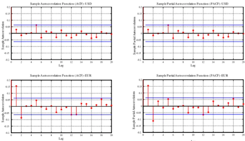
correlations for returns in Figure 2 were evaluated with autocorrelation functions (ACF) and partial autocorrelation functions (PACF). Here, it was observed that all autocorrelations were not zero after zero lag. Since …nancial returns are considered to be time series data, their marginal distributions were regarded as GARCH and GJR models.
Table 1. Descriptive statistics and tests
Statistics USD EUR
Sample number 1007 1007
Mean 0.0400 0.0314
Standart deviation 0.6061 0.5945
Skewness 0.2363 -0.0421
Kurtosis 2.8009 4.6870
Tests Q-stat. p-value Q-stat. p-value
Jarque-Bera 333.8726 0.0001 910.5830 0.0001 Engle-ARCH LM(4) 85.6759 0.0000 100.2175 0.0000 LM(6) 90.2060 0.0000 101.2061 0.0000 LM(8) 96.7109 0.0000 101.1312 0.0000 LM(10) 96.7643 0.0000 101.0680 0.0000 0 2 4 6 8 10 12 14 16 18 20 -0.2 -0.15 -0.1 -0.05 0 0.05 0.1 0.15 0.2 Lag S am pl e A ut oco rr el at io n
Samp le Au to co rrelatio n Fu n ctio n (ACF)-USD
0 2 4 6 8 10 12 14 16 18 20 -0.2 -0.15 -0.1 -0.05 0 0.05 0.1 0.15 0.2 Lag S am ple P ar tia l A ut oc or re la tions
Samp le Partial Au to co rrelatio n Fu n ctio n (PACF)-USD
0 2 4 6 8 10 12 14 16 18 20 -0.2 -0.15 -0.1 -0.05 0 0.05 0.1 0.15 0.2 Lag S am pl e A ut oco rr el at io n
Samp le Au to co rrelatio n Fu n ctio n (ACF)-EUR
0 2 4 6 8 10 12 14 16 18 20 -0.2 -0.15 -0.1 -0.05 0 0.05 0.1 0.15 0.2 Lag S am ple P ar tia l A ut oc or re la tions
Samp le Partial Au to co rrelatio n Fu n ctio n (PACF)-EUR
Figure 2. Autocorrelations USD and EUR indexes and partial autocorrelation measurements
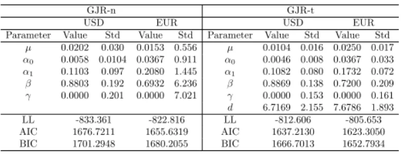
It was determined by goodness of …t tests that the marginal distributions of the USD and the EUR is the best appropriated by GARCH (Normal, Student-t) or GJR (Normal, Student-t) models. Table 2 and Table 3 show that maximum likelihood results, estimated parameter values, AIC (Akaike Information Criterion) and BIC (Bayesian Information Criterion) values for GARCH and GJR models selection. It is demonstrated that both the USD and EUR can be modeled with GARCH-t since it has minimum AIC and BIC values.
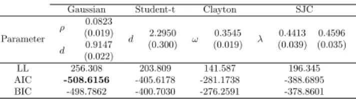
In order to explain the dependency structure of USD and EUR, the best copula models were selected by using the estimated parameter values for the identi…ed marginal distributions. The copula selection model was examined in two situa-tions: static (Gaussian, Student-t, Clayton, SJC) and dynamic (GDCC, tDCC, tvC, tvSJC). Table 4 and Table 5 demonstrate the AIC and BIC values besides the estimated parameter results by the IFM method for these situations. Thus, the Gaussian copula and tDCC copula are selected for static and dynamic cases, respectively, since they have minimum AIC and BIC values. By using the para-meter values for selected model, the Monte Carlo simulation was performed 10000 times, and portfolio optimization was achieved based on CV aR. V aR and CV aR risk measurement values for di¤erent con…dence levels, and results including the weights for each …nancial asset are given in Table 6. Accordingly, the CV aR value would reach the minimum when an investor allocates of his/her assets 37% in USD and 63% in EUR within a 99% con…dence level.
Table 2. Parameter estimates of GARCH-n, and GARCH-t models and
statistic tests
GARCH-n GARCH-t
USD EUR USD EUR
Parameter Value Std Value Std Parameter Value Std Value Std 0.0202 0.015 0.0153 0.019 0.0104 0.014 0.0250 0.017 0 0.0058 0.006 0.0367 0.015 0 0.0047 0.004 0.0367 0.018 1 0.1102 0.049 0.2080 0.066 1 0.1082 0.045 0.1732 0.064 0.8803 0.057 0.6932 0.092 0.8867 0.047 0.7200 0.107 d 6.7220 1.266 7.6785 1.700 LL -833.360 -822.816 LL -812.607 -805.652 AIC 1674.7207 1653.6311 AIC 1635.2130 1621.3042 BIC 1694.3797 1673.2901 BIC 1659.7867 1645.8779
Table 3. Parameter estimates of GJR-n and GJR-t models and statistic tests
GJR-n GJR-t
USD EUR USD EUR
Parameter Value Std Value Std Parameter Value Std Value Std 0.0202 0.030 0.0153 0.556 0.0104 0.016 0.0250 0.017 0 0.0058 0.0104 0.0367 0.911 0 0.0046 0.008 0.0367 0.033 1 0.1103 0.097 0.2080 1.445 1 0.1082 0.080 0.1732 0.072 0.8803 0.192 0.6932 6.236 0.8869 0.138 0.7200 0.209 0.0000 0.201 0.0000 7.021 0.0000 0.153 0.0000 0.161 d 6.7169 2.155 7.6786 1.893 LL -833.361 -822.816 LL -812.606 -805.653 AIC 1676.7211 1655.6319 AIC 1637.2130 1623.3050 BIC 1701.2948 1680.2055 BIC 1666.7013 1652.7934
Table 4. Parameter estimates for static copula families and model se-lection statistics
Gaussian Student-t Clayton SJC
Parameter d 0.0823 (0.019) 0.9147 (0.022) d 2.2950 (0.300) ! 0.3545 (0.019) 0.4413 0.4596 (0.039) (0.035) LL 256.308 203.809 141.587 196.345 AIC -508.6156 -405.6178 -281.1738 -388.6895 BIC -498.7862 -400.7030 -276.2591 -378.8601
Table 5. Parameter estimates for dynamic copula families and model
selection statistics GDCC tDCC tvC tvSJC Parameter 0.0823 (0.019) 0.9147 (0.022) d 3.9987 (0.739) 0.0524 (0.014) 0.9473 (0.015) ! 0.1419 (0.051) -0.7605 (0.283) 0.9523 (0.017) -0.7380 0.1631 (0.279) (0.056) 0.9651 1.1030 (0.012) (0.278) -5.6345 0.8175 (1.356) (0.083) LL 256.308 274.546 200.593 256.543 AIC -508.6156 -543.0916 -395.1857 -501.0861 BIC -498.7862 -528.3475 -380.4415 -471.5977
Table 6. The results of portfolio optimization based on CV aR for full sample
Full Sample GARCH(1,1)-t, tDCC V aR CV aR x1 U SD x2 EU R %90 0.4078 0.8321 0.4245 0.5755 %95 0.6770 1.1460 0.4209 0.5791 %99 1.4307 1.9740 0.3716 0.6284
Table 7. Change point dates and events
Periods Dates Events Change Points
I 03.01.2011-14.12.2011
-II 15.12.2011-14.05.2013 America withdrew from Iraq 15.12.2011
III 15.05.2013-14.07.2013 FED decision 15.05.2013
IV 15.07.2013-28.01.2014 TCMB announced that
they may consider raising interest rates at MPC meeting 15.07.2013
V 29.01.2014-20.05.2014 MPC increased interest rates 29.01.2014
VI 21.05.2014-07.09.2014 Speech of FED Chairman 21.05.2014
VII 08.09.2014-31.12.2014 FED decreased interest rates. 08.09.2014
Table 7 presents change point dates (periods) and events which are obtained with the change point approach. The parameter estimates of GARCH (1,1)-t for periods are calculated and presented in Table 8. The estimates of static and dynamic copula parameters for each period are given in Table 9 and Table 10, respectively. Finally, portfolio optimization for these periods are carried out and the results are given Table 11.
Table 8. Estimate of GARCH (1,1)-t parameters for sample periods by change point approach
Parameters Periods Currency 0 1 d I USD 0.0641 0.0302 0.0743 0.8680 28.6263 EUR 0.0964 0.0524 0.0940 0.7905 7.0189 II USD -0.0056 0.0009 0.0467 0.9448 13.9576 EUR -0.0124 0.0067 0.0256 0.9332 172.7160 III USD 0.1632 0.0303 0.0000 0.9315 3.6763 EUR 0.2024 0.0079 0.0564 0.9436 39.3986 IV USD 0.1030 0.0498 0.2106 0.7186 5.2203 EUR 0.1265 0.0522 0.4250 0.5396 6.2406 V USD -0.1098 0.0587 0.1688 0.6834 5.6044 EUR -0.1083 0.0587 0.0885 0.7516 4.9476 VI USD -0.0060 0.0189 0.2406 0.7184 4.4100 EUR -0.0458 0.0229 0.1389 0.7656 5.5815 VII USD 0.0391 0.0417 0.0000 0.9128 3.4960 EUR -0.0158 0.0417 0.0000 0.9031 3.3790
Table 9. Estimates of static copula parameters by change points approach
Periods Static Change Time
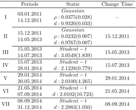
I 03:01:2011 14:12:2011 Gaussian : 0:0375(0:028) d : 0:9320(0:033) -II 15:12:2011 14:05:2013 Gaussian : 0:0232(0:007) d : 0:9767(0:007) 15.12.2011 III 15:05:2013 14:07:2013 Student t d : 3:0549(1:839) 15.05.2013 IV 15:07:2013 28:01:2014 Student t d : 2:1228(0:779) 15.07.2013 V 29:01:2014 20:05:2014 Student t d : 2:0100(4:265) 29.01.2014 VI 21:05:2014 07:09:2014 Student t d : 2:0102(10:723) 21.05.2014 VII 08:09:2014 31:12:2014 Student t d : 2:2983(1:050) 08.09.2014
Table 10. Estimates of dynamic copula parameters by change points approach
Periods Dynamic Change Time
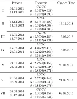
I 03:01:2011 14:12:2011 GDCC : 0:0375(0:028) : 0:9320(0:033) -II 15:12:2011 14:05:2013 tDCC d : 8:4731(5:300) : 0:0209(0:008) : 0:9763(0:006) 15.12.2011 III 15:05:2013 14:07:2013 GDCC : 0:5000(0:286) : 0:1137(0:121) 15.05.2013 IV 15:07:2013 28:01:2014 tDCC d : 3:4672(2:412) : 0:2425(0:165) : 0:2442(0:288) 15.07.2013 V 29:01:2014 20:05:2014 tDCC d : 2:7274(0:455) : 0:0222(0:028) : 0:8308(0:071) 29.01.2014 VI 21:05:2014 07:09:2014 tDCC d : 2:5263(0:641) : 0:0290(0:040) : 0:8308(0:071) 21.05.2014 VII 08:09:2014 31:12:2014 GDCC : 0:0000(0:257) : 0:4958(4:044) 08.09.2014
Table 11. The results of portfolio optimization based on CV aR for
change points = %95 GARCH(1,1)-t, tDCC Periods V aR CV aR x1 U SD x2 EU R I 0.9434 1.2783 0.4080 0.5920 II 0.6109 0.8201 0.2104 0.7896 III 0.4170 0.5840 0.8215 0.1785 IV 1.1101 1.6882 0.5569 0.4431 V 0.0500 6.3605 0.1051 0.9949 VI 1.0813 1.4849 0.2442 0.7558 VII 0.5386 0.6853 0.4612 0.5388
6. CONCLUSION AND DISCUSSION
In this paper, we constructed a dynamic copula model for currency data (USD and EUR) with the change point approach. This study was conducted in two cases: Full sample and subsamples by change point aprroach. In the …rst case, marginal distributions were determined as GARCH-t and the best copula describing the de-pendence structure of currency data was found as Gaussian in the static model and tDCC in the dynamic model. In the second case, the full sample was divided into subsamples (periods) with the change point approach. This approach allows us to determine the change points for the types of copulas using the binary segmentation method. Thus, seven periods are obtained to study on. Marginal distributions and appropriate copula models are determined for each period. Then, optimization based on CV aR by using Monte Carlo simulation was performed for full sample and seven periods. As result, it was seen how the copula models and their parameters changed from period to period. Therefore, the portfolio optimization results were obtained for each period and it was found the best way to allocate portfolio assets. As it can be inferred from the results of the numerical example, copula models may subject to change according to some political or …nancial events during the time schedule which may a¤ect the future structure of investment strategies.
In future work, it is possible to study other copula families for another …nancial investment instruments by taking into account the change point approach.
7. APPENDIX
The used static copulas in this paper are given as follows: Gaussian Copula
De…ning x = 1(u) and y = 1(v) , the Gaussian copula is given by
CGau(u; v; ) = x Z 1 y Z 1 1 2 p1 2exp( x2 2 xy + y2 2(1 2) )dxdy
with 2 ( 1; 1); where 1is the inverse of the normal c.d.f. and is the coe¢ cient of linear correlation. The Gaussian copula has no tail dependence. The Clayton copula is also Archimedean, but it is not rotationally symmetric and it only allows for positive dependence [5,6,16].
Student t Copula
De…ning x = td1(u) and y = td1(v) , the Student-t copula is given by
CStudent(u; v; ; d) = x Z 1 y Z 1 1 2 p1 2exp(1 + x2 2 xy + y2 d(1 2) )dxdy
where td1 is the inverse of a Student-t c.d.f., the parameters 2 ( 1; 1) and d 2 (0; 1) are the coe¢ cient of linear correlation and the degrees of freedom, respectively [5,6,16].
Clayton copula The Clayton copula is
CClayton(u; v; w) = (u w+ v w 1)
1 w
with w 2 (0; 1). The Clayton copula is also Archimedean, but it is not rotationally symmetric and it only allows for positive dependence [5,6].
The symmetrized Joe-Clayton (SJC) Copula
The Joe-Clayton copula is constructed by taking a particular Laplace transfor-mation of Clayton’s copula by Joe [4] and it is given by
CJ C u; vj U; L = 1 1 n [1 (1 u) ] + [1 (1 v) ] 1o 1= 1= with = 1 log2(2 U) and = 1
log2( L). The symmetrized Joe-Clayton (SJC) copula is improved by Patton [27], in order to overcome the asymmetry property of the Joe-Clayton copula, when U = L, and this copula is de…ned by
CSJ C(u; v; w) = 1
2 CJ C u; vj
U; L + C
J C 1 u; 1 vj L; U + u + v 1 which is symmetric when U = L. The parameters U 2 (0; 1) and L 2 (0; 1) are the coe¢ cients of upper and low tail dependence, respectively.
References
[1] Akaike, H., A new look at the statistical model identi…cation, Automatic Control, IEEE Transactions on (1974), 19, 716-723.
[2] Schwarz, G., Estimating the dimension of a model, Annals of Statistics (1978), 6, 461-464. [3] Emrechts, P., McNeil, A. and Straumann D., Correlation and dependence in risk
manage-ment: properties and pitfalls, In Risk Management Value at Risk and Beyond (Edited by M. Dempster) (2002), 176-223, (Cambridge University Press).
[4] Joe, H., Multivariate Models and Dependence Concepts, Chapman & Hall/CRC, London 1997.
[5] Nelsen, R.B., An Introduction to Copulas, (second ed), Springer, New York, 2006.
[6] Cherubini, U., Luciano, E. and Vecchiato, W., Copula Methods in Finance, John Wiley and Sons, New York, 2004.
[7] Wei, Y. and Zhang, S., Multivariate Copula-GARCH Model and Its Applications in Financial Risk Analysis [J], Application of Statistics and Management (2007), 3, 008.
[8] Ozun, A., Cifter, A.,Portfolio value-at-risk with time-varying copula: Evidence from the Americans, Marmara University (2007), MPRA Paper No. 2711.
[9] Jondeau, E., and Rockinger, M., The copula-garch model of conditional dependencies: An international stock market application. Journal of international money and …nance (2007), 25(5), 827-853.
[10] Huang, J. J., Lee, K. J., Liang, H. and Lin, W.F., Estimating value at risk of portfolio by conditional copula-GARCH method, Insurance: Mathematics and Economics (2009), 45, 315- 324.
[11] Rockafellar, R. T. and Ursayev, S., Optimization of conditional value at risk, Journal of Risk (2002), 2, 21-40.
[12] Wu, Z.X., Chen, M. and Ye, W.Y., Risk Analysis of Portfolio by Copula-GARCH, Journal of Systems Engineering Theory and Practice (2006), 2(8), 45-52.
[13] Wang, Z. R., Chen, X. H., Jin, Y. B., Zhou, Y.J., Estimating risk of foreign exchange portfolio: Using V aR and CV aR based on GARCH-EVT-Copula model, Physica A (2010), 389, 4918-4928.
[14] He, H., Li, P., Dynamic asset allocation based on copula and CV aR. International Conference on. IEEE (2011), 1-4.
[15] Gombay, E., and Horváth, L., On the rate of approximations for maximum likelihood tests in change-point models, Journal of Multivariate Analysis (1996), 56(1), 120-152.
[16] Gombay, E., and Horvath, L., Change-points and bootstrap, Environmetrics (1999), 10(6), 725-736.
[17] Cs½org½o, M., Horváth, L., Limit Theorems in Change-point Analysis,Wiley: Chichester, 1997. [18] Zhu, X., Li, Y., Liang, C., Chen, J., Wu, D., Copula based Change Point Detection for
Financial Contagion in Chinese Banking. Procedia Computer Science (2013), 17, 619-626. [19] Dias, A., and Embrechts, P., Change-point analysis for dependence structures in …nance
and insurance, Novos Rumos em Estatistica (Ed. C. Carvalho, F. Brilhante and F. Rosado), Sociedade Portuguesa de Estatstica, Lisbon (2002), 69-86.
[20] Dias, A., and Embrechts, P., Dynamic copula models for multivariate high-frequency data in …nance. Manuscript, ETH Zurich, 2004.
[21] Guegan, D., and Zhang, J., Change analysis of a dynamic copula for measuring dependence in multivariate …nancial data. Quantitative Finance (2010), 10(4), 421-430.
[22] Sklar, A., Functions De Repartition An Dimensions At Leurs Marges, Publications De L’¬nstitut De Statistique De L’université De Paris (1959), 8, 229-231.
[23] Bollerslev, T., Generalized autoregressive conditional heteroskedasticity, (1986), Journal of econometrics, 31 (3), 307-327.
[24] Genest, B. Rémillard, D. Beaudoin., Goodness-of-…t tests for copulas: A review and a power study. Mathematics and Economics (2009), 44, 199-213.
[25] Vostrikova, L. J., Detecting "disorder" in multidimensional random processes. Soviet Math-ematics Doklady, 1981, 24, 55-59.
[26] http://evds.tcmb.gov.tr/cbt.html [12.01.2015].
[27] Patton, A., Modelling Asymmetric Exchange Rate Dependence. International Economic Re-view (2006), 47(2), 527-556.
Current address : Emel KIZILOK KARA, Kirikkale University, Faculty of Arts and Sciences, Department of Actuarial Science, Kirikkale - TURKEY
E-mail address : [email protected]
Current address : Sibel ACIK KEMALOGLU Ankara University, Faculty of Sciences, Depart-ment. of Statistics, Ankara, TURKEY (Corresponding Author)