© TÜBİTAK
doi:10.3906/elk-1809-190
h t t p : / / j o u r n a l s . t u b i t a k . g o v . t r / e l e k t r i k / Research Article
Consumer loans’ first payment default detection: a predictive model
Utku KOÇ1,2,∗, Türkan SEVGİLİ21Department of Industrial Engineering, Faculty of Engineering, MEF University, İstanbul, Turkey 2Graduate School of Science and Engineering, MEF University, İstanbul, Turkey
Received: 26.09.2018 • Accepted/Published Online: 10.09.2019 • Final Version: 27.01.2020
Abstract: A default loan (also called nonperforming loan) occurs when there is a failure to meet bank conditions and repayment cannot be made in accordance with the terms of the loan which has reached its maturity. In this study, we provide a predictive analysis of the consumer behavior concerning a loan’s first payment default (FPD) using a real dataset of consumer loans with approximately 600,000 records from a bank. We use logistic regression, naive Bayes, support vector machine, and random forest on oversampled and undersampled data to build eight different models to predict FPD loans. A two-class random forest using undersampling yielded more than 86% on all performance measures: accuracy, precision, recall, and F1-score. The corresponding scores are even as high as 96% for oversampling. However, when tested on the real and balanced dataset, the performance of oversampling deteriorates as generating synthetic data for an extremely imbalanced dataset harms the training procedure of the algorithms. The study also provides an understanding of the reasons for nonperforming loans and helps to manage credit risks more consciously.
Key words: Machine learning, default loan, first payment default, imbalanced class problem, oversampling, undersam-pling
1. Introduction and literature review
Technological advances and increase in computing power and data availability lead to the use of big data analytics in many areas including language processing, image recognition, and fraud detection. Banks and lending institutions are actively using analytics in predicting credit risks and monitoring the loans. The use of analytical tools results in reliable, transparent, and objective decision making procedures.
In the past decade, a rapid expansion of consumer loans has been witnessed, which is profitable but risky for banks. Banks have made great efforts to develop numerous analytic models to identify potential default loan applicants, control risk, and maximize profits. These models would help the bank avoid loan loss, improve the performance, and maximize the efficiency. Because consumer credit is a remunerative business, the banks do not want to refuse those who will not default. For this reason, banks want to understand their existing customers and classify the common features of nonperforming customers. They want to correctly guess the potential default customers from loan applications. Therefore, in credit-risk analysis, estimating default risk has been a major challenge.
Loan default can be basically explained as that money allocated by the bank cannot be repaid in accordance with the terms of the loan. It can also be called an unrequited loan. The target is to minimize the ∗Correspondence: [email protected]
risk of having a loan loss. One of the most important measurements to assess the strength of a bank is to assess the performance of the organization’s loan portfolio loss by estimating the likelihood of default (probability of a loan that will go into default or not). This is very important for risk management and credit risk analysis.
In finance terminology, a default loan (also called a nonperforming loan) is a failure to meet conditions and the loan cannot be repaid in accordance with the terms of the loan which has reached its maturity. For instance, when a customer who has a debt that has a due date to pay and the customer has passed the payment deadline, a default occurs. Consumer default frequently occurs in credit card payments, mortgage payments, or consumer loans. If no payment is made within the period even though the bank has served a notice of maturity to the customer, then it is regarded that the customer has gone into default. The first payment default (FPD) definition is crucial for our study. FPD occurs when loan applicants are likely to be late making their first payment on a consumer loan. A bank usually wants to be able to predict which applicants who have been granted loans are likely to default on the loans, by predicting the FPD.
Although the use of machine learning techniques in fraud detection has spread rapidly, using machine learning algorithms to predict defaults in consumer loans is a relatively new concept and as such related literature is quite limited.
The literature on logistic regression (LR) reveals that LR, as a predictive model, is widely used in classification and forecast phenomena. LR is a regression method where the target variable is a nonlinear function of the probability of being classified as a certain class [1]. Moreover, according to the study, the classification results of the LR model are sensitive to correlations between the independent variables. The regression coefficients are usually estimated using maximum likelihood estimation [2]. When taking a note from the article by King and Zeng [3], many researchers are concerned about whether the use of traditional logistic regression is legitimate for rare events. The difficulty is not specifically the rarity of events, rather possibility of a few numbers of cases on the more unusual of the two results.
Machine learning has been extensively studied in different fields (e.g., speech recognition, pattern recogni-tion, image classificarecogni-tion, and natural language processing). Similarly, machine learning has also been employed to predict defaults in consumer and commercial loans. Technological developments made it easy to handle large amounts of data. Our study is a shift from the previous (public) machine learning studies on consumer loans as our dataset consist of extensive amounts of real data.
Other machine learning-based studies conducted to predict defaults in consumer loans include Khandani et al. [4], Butaru et al. [5], and Fitzpatrick and Mues [6]. Khandani et al. [4] used generalized classification and regression trees to construct nonlinear, nonparametric forecasting models of consumer credit risk by combining customer transactions and credit bureau scores. Butaru et al. [5] applied logistic regression, decision trees using the C4.5 algorithm, and the random forests methods to combined consumer trade-line, credit-bureau, and macroeconomic variables to predict delinquency. Fitzpatrick and Mues evaluated the performance of logistic regression, semiparametric generalised additive models, boosted regression trees, and random forests for future mortgage default status [6]. These studies aim to give an overview of the objectives, techniques, and difficulties of credit scoring as an application of forecasting. Our study is quite different from these studies in that we examine and focus only on FPD loans. The importance of analyzing the default loans stems from the fact that increase in default loans subsequently has an impact on credit shrinkage (reduction in credit volume).
Recently, Addo et al. used elastic net, random forest, gradient boosting, and deep learning to predict the defaults for commercial credits [7]. Their study considered around 110,000 lines with 235 variables to predict a commercial loan to be default or not.
Tang et al. used random forest algorithm to assess the risk of energy industry in China [8]. Their study is based on around 25,000 credit card data on energy industry. In another example, Tsai et al. [9] predicted the defaults in consumer loans based on a small sample of 350 loans.
The originality of the present study stems from two facts: 1) This is the first public study that considers a large amount of real data. The banks monitor and control the default risks privately, and tend not to disclose related material to the public. Public studies do not consider extensive amounts of real data and rather focus on small samples or commercial side; 2) Related literature generally mentions default risk and risk management unlike the first payment default. To the best of our knowledge, this study is the first FPD prediction study applied and tested on a real dataset with an extensive amount of data in Turkey.
2. Data and preprocessing
This study is a data mining attempt in the analysis of FPD loan applicants using a real dataset consisting of nearly 600 K observations obtained from a bank. The data have been collected from a Turkish bank’s database system with direct access via SQL. The dataset of the study consists of the underlying consumer loans’ (not all individual credits) information that concerns only the allocated loans for the period from January 2017 to November 2017. Dataset consists of 45 columns and 598,669 rows each of which represents a consumer loan’s details. Each observation includes sex, age, education, occupation, marriage status, housing status, household income, and bank’s classification of one client of the bank, and loan details. There is a target value that represents FPD flag of a consumer loan. If there is a first payment default the “FPD_flag” is 1 otherwise 0.
The distribution of the two classes (FPD and non-FPD) in the dataset is imbalanced. Out of 598,669 observations, more than 99.5% (595,963) are defined as non-FPD while less than 0.5% of the data is assigned to the FPD loan class. Thus, classifiers might not be able to recognize minor classes and are influenced by major classes. Before applying the model, the data need to be balanced. We use two resampling methods, namely, oversampling and undersampling, to balance the data.
In the Turkish banking sector, individual loans include credits for automobiles, mortgages, and individual consumption credits (which is referred to as consumer loans in this study). However, most of the consumer loans are individual consumption credits. Thus, this type of credit was selected in this study. According to the Main Indicators Report released in December 2017 published by the Banking Regulation and Supervision Agency, the share of the individual loans was 41%, the percentage of mortgages was 39%, and the percentage of credit cards was 19%. In the Turkish banking sector, the default conversion rate of the loans was 2.96% in the December 2017 period. This rate is slightly higher on individual loans. As of December 2017, the amount of nonperforming loans (gross) was 18 billion TRY (equivalent to $5 billion) [10].
2.1. Exploratory data analysis
In this section, we provide a descriptive analysis of the variables used in the study, to get a general understanding and to identify relevant variables. We note that the number of FPD loans (the target variable) is much lower than that of timely/early paid loans. Only 0.45% of all the loans are marked as FPD. This is because all banks are using other methods to prevent loan losses. Thus, it is expected to have a low ratio of nonperforming loans. Analyzing the descriptive statistics, we observe that the majority (about 72%) of loan applicants are male. According to the Labor Force Statistics published by the Turkish Statistical Institute (TSI), the labor force participation rate is 71.5% for males and 33.3% for females [11]. This statistic shows that males manage the
economy of the family in Turkey and it is a reflection of male dominated society. According to the Address Based Population Registration System Results provided by TSI, in 2017, it is known that the population over 15 years old is about 61 million, of which 63.37% is married [12]. The ratio of married applicants is 65% in our dataset. According to the National Education Statistics Database provided by TSI, in 2017, the highest proportions with respect to education is primary school education with 38% and high school with 23% [12]. We observe that 40% of the loan applicants are high school graduates, and approximately 33% of all applicants are primary and secondary school graduates. This suggests that average education level of the consumer loan applicants is higher than that of the general public.
2.2. Preprocessing of data
One of the challenges in solving real life applications is acquiring a reliable and clean dataset. Recall that the scope of this study is only the consumer loans. Banks use the same system to record the data for all types of loans. Hence, some columns may not be needed for consumer loans. Moreover, the relevant data for loan applications is entered manually by alternative channels and employees over a long period of time.
As a first step, we eliminated the features for which at least 25% of the data is missing. We also conjecture that these variables have little or no value in predicting FPD status. The columns eliminated because of high missing value percentages are work phone, city of work, net monthly expense, status of military service, and staff code.
The features distinguishing the loan type, customer type, and loan status are the same for all data points in this study. These columns have no value; hence, they are excluded. Columns that identify the client (name, id card number, loan id) are also excluded as they are confidential and/or irrelevant.
In the dataset, the columns that represent clients’ preexisting information about the loans are also excluded. These include the payment and lateness status of all payments for the loan. A new consumer loan cannot have the payment information during the loan application phase.
Allocated loan amount and loan amount with interest columns have almost the same information (one being the interest-free value of the other). To avoid the adverse effects of multicollinearity, we only kept one of the variables, i.e. the loan amount. Some other columns such as branch code and campaign number are also discarded based on similar reasons.
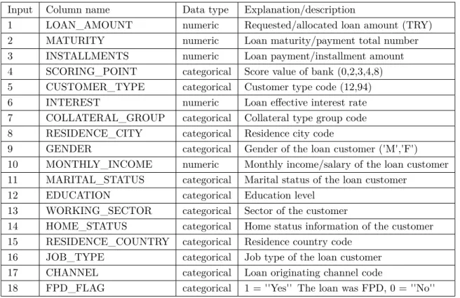
The performance of the machine learning algorithms may be adversely effected if the values of the independent variables are very low or very high. A common approach to get all variables in an equivalent range is scaling. In this study, we used MinMax scaler in the preprocessing phase to transform the values for each numerical variable to be between 0 and 1. Specifically, we used the MinMax scaler for the following variables: allocated loan amount, loan installment amount, loan effective interest rate, and monthly income/salary. After the preprocessing phase, the dataset includes 17 independent variables to predict the categorical FPD variable. Table1provides a summary of the variable names, types (numerical/categorical), and short descriptions included in the study.
We would like to note that all the loans in our dataset are already accepted loans. As banks use multiple methods in the application process, only a small fraction of the loans are FPD. Moreover, it is not possible to follow a rejected application in terms of being FPD or not, as the application is rejected in the first place. Hence, the dataset consists of rare events of being FPD.
Table 1. Variables included in the analysis.
Input Column name Data type Explanation/description
1 LOAN_AMOUNT numeric Requested/allocated loan amount (TRY)
2 MATURITY numeric Loan maturity/payment total number
3 INSTALLMENTS numeric Loan payment/installment amount
4 SCORING_POINT categorical Score value of bank (0,2,3,4,8)
5 CUSTOMER_TYPE categorical Customer type code (12,94)
6 INTEREST numeric Loan effective interest rate
7 COLLATERAL_GROUP categorical Collateral type group code
8 RESIDENCE_CITY categorical Residence city code
9 GENDER categorical Gender of the loan customer ('M','F')
10 MONTHLY_INCOME numeric Monthly income/salary of the loan customer
11 MARITAL_STATUS categorical Marital status of the loan customer
12 EDUCATION categorical Education level
13 WORKING_SECTOR categorical Sector of the customer
14 HOME_STATUS categorical Home status information of the customer
15 RESIDENCE_COUNTRY categorical Residence country code
16 JOB_TYPE categorical Job type of the loan customer
17 CHANNEL categorical Loan originating channel code
18 FPD_FLAG categorical 1 = ''Yes'' The loan was FPD, 0 = ''No''
3. Methodology
In the supervised learning framework, the learner algorithm is presented with input/output pairs from the past data, in which the input data represent preidentified attributes to be used to determine the output value [4]. We use supervised learning algorithms since our problem serves as a binary classification problem, being FPD or not. Alternative machine learning algorithms can be applied to predict FPD loans. It is conjectured that the forecast performances of nonlinear and nonparametric algorithms are better than the conventional models [13]. In this study, we use four classification algorithms: logistic regression (LR), naive Bayes classifier (NBC), random forest (RF), and support-vector machines (SVM) algorithms. In total, we apply eight different models based on these four machine learning algorithm approaches and compare their performances. These models are suitable for loan level analysis as the size of the dataset is large enough to capture the complex relationships among features. The categorical variables are converted to numerics for SVM and LR methods.
Logistic regression is a parametric algorithm that considers the linear connections between the predictors and the classes. Moreover, these regressions measure the effect of changes in a predictor on the response, which is independent of the values of the other predictors. Logistic models are suitable to model consumer loans being FPD or non-FPD, as the performance status of a consumer loan is a qualitative probability value represented by categorical variables. In the simplest terms, logistic regression estimated the probability that a certain input
x belongs to class 1, by using a sigmoid function a = 1
1+e−(wT x+b) of linear transformation of x . Here, w and
x are in the input dimensions and b is referred to as the bias. If the calculated probability is greater than
is classified as class 0. The parameters w and b are calculated in such a way to minimize the prediction error ∑
iy
ilog(ai) + (1− yi)log(1− ai) , where yi is the actual output and ai= 1
1+e−(wT xi+b) is the probability that input xi belongs to class 1.
Naive Bayes classifiers are widely used classification algorithms. They assume an underlying probabilistic model (Bayes’ theorem) with simple, robust, strong, and naive independence assumption between the features. Naive Bayes classifiers are conditional probabilistic models that include a decision rule.
Given an n dimensional data point x , naive Bayes predicts the class Ck for x according to the probability
P (Ck|x). Using the Bayes’ theorem P (Ck|x) = P (x|CP (x)k)P (Ck) = P (x1,...,xP (xn|Ck)P (Ck)
1,...,xn) . Using the chain rule, and
by the naive assumption of independence of the xi’s, the factor P (x1, . . . , xn|Ck) can be calculated by
P (x1, . . . , xn|Ck) = P (x1|x2, . . . , xn, Ck)P (x2|x3, . . . , xn, Ck) . . . P (xn−1|xn, Ck)P (xn|Ck)
Naive Bayes gives the probability of a data point x belonging to class Ck as proportional to a simple
product of the class prior probability ( P (Ck) ) of n conditional feature probabilities. The point is assigned to
the class k with the greatest P (Ck|x) value. Support-vector machines (SVMs) are one of the best learning
algorithms for classification and regression. They seek to find hyperplanes that separate the data as good as possible. Additionally, there are many hyperplanes that can separate the classes and each of them has a certain margin. The distance between observations and the decision boundary explains the quality of prediction. The more distant an observation is to a hyperplane, the higher the probability of correct classification is. Hence, an optimal hyperplane maximizes the margin. These optimal hyperplanes determined based on the observations within the margin are called the support vectors.
In mathematical terms, SVM tries to find a hyper-plane (w, b) such that all points in xn belonging to
negative class (class 0) satisfy wTx + b≤ −1 and all points in x
p belonging to positive class (class 1) satisfy
wTx + b≥ 1. Here wTx + b =−1 is the negative classification boundary and wTx + b = 1 is the positive class
boundary. The margin M between these boundaries is M = 1
||w||. In order to maximize the margin M , the
following optimization problem is solved
min||w|| : y(wTx + b)≥ 1.
Decision tree is a simple to implement and easy to understand algorithm which is suitable for forecasting, especially when the dataset is imbalanced. It can also be used when the training data contain missing observations and/or outliers. However, tree learners have a lower prediction performance in comparison to other machine learning algorithms as they have restricted capacity in generalizing the results and handling large number of variables. A decision tree is a hierarchical data structure composed of decision nodes and leaves (terminal). Each decision node m implements a test function fm(x) with discrete outcomes labeling the
branches. At each iteration of the algorithm the goodness of a split is quantified by an impurity measure. The most common measures used for classification are entropy (∑k−fklog2fk) and gini impurity (
∑
k−fk(1−fk) ),
where fk is the frequency of label k at the given node. Random forests (RF) are constructed by generating
3.1. Sampling methods
Studies have shown that standard classifiers have better performances when trained on balanced sets [14]. As our dataset is not balanced, we use resampling methods for balancing the dataset. These techniques do not consider class information in removing or adding observations. As the number of FPD loans is much lower than the non-FPD loans, we use both undersampling and oversampling to build efficient models with high accuracy. Undersampling balances the data by downsizing the majority class. Observations in the majority class are randomly deleted until the frequency of the classes are similar. However, the loss of data points leads to the loss of information, which is of utmost value. As the size of the remaining set is relatively small, it is possible to get quick results by working on the undersampled dataset.
Oversampling upsizes the minority class by replicating the data points until the frequencies of the two classes are similar. One drawback of this approach is the increased risk of overfitting, as the data is now biased towards the minority class.
Synthetic minority oversampling technique (SMOTE) is an oversampling algorithm which upsizes the minority class by generating synthetic examples in the neighborhood of observed ones. It forms new minority examples by interpolating between samples of the same class instead of replicating [15]. This reduces the risk of overfitting and and creates clusters around each minority observation. It is shown that SMOTE improves the performances of the base classifier in many applications. In our study we use both under- and oversampling methods.
3.2. Evaluation metrics
The performance of the multiple models tested on alternative resampled data may vary. One of the aims of this study is to assess the performance of alternative machine learning algorithm. In order to assess the performance differences amongst algorithms, we calculate four metrics: accuracy, precision, recall, and F1-score. For all algorithms, we split the data into train/test, where the training set is used to calculate algorithm parameters and test set is used to evaluate the performance of the algorithms. For each method, we also share the test results via the confusion matrices—a table that shows the number of true-positives (TP), false-positives (FP), true-negatives (TN), and false-negatives (FN).
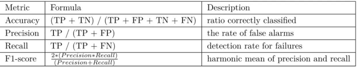
The performance of each model was examined by computing the aforementioned four metrics. A widely used metric, accuracy, is the fraction of predictions the model correctly determines (i.e. number of correct predictions/total number of predictions). Accuracy does not provide a fair comparison among multiple methods, especially for imbalanced datasets. We compared the models based on well-known and commonly used metrics such as precision, the rate of false alarms; recall, detection rate of failures; and F1-score, the harmonic mean of precision and recall. All metrics are calculated using the TP, FP, FN rates. Table 2 summarizes the metrics, their formulas, and descriptions used in the study.
Table 2. Evaluation metrics.
Metric Formula Description
Accuracy (TP + TN) / (TP + FP + TN + FN) ratio correctly classified
Precision TP / (TP + FP) the rate of false alarms
Recall TP / (TP + FN) detection rate for failures
F1-score 2∗(P recision∗Recall)
A K-fold cross-validation procedure is also used to evaluate each algorithm. In a K-fold cross-validation approach, the data is randomly split into K subsets of equal size. The algorithm is run K times, each subset is used once as the test set, and K-1 times as a part of the training set. The evaluation metrics are calculated as the average of the K folds.
4. Results
The FPD loans in the dataset constitute a very small percentage of the data and this makes the dataset imbalanced. Working on imbalanced data without resampling may lead to wrong conclusions. Recall that only 0.45% of all the loans is FPD. Any algorithm can get an accuracy of 99.55% by marking all loans classified as non-FPD. Traditional machine learning algorithms may influence the classifier, which will be tended to favor the majority class. This results in poor predictive accuracy for the minority class due to the number of occurrences being low. Thus, we run all the algorithms on both undersampled and oversampled datasets. In the undersampling case, we create a new dataset with a total of 5412 loans, 2706 instances being in Class 0 (Non-FPD) and 2706 instances being in Class 1 (FPD). For oversampling, we used SMOTE with a percentage parameter as 20,000%. In the oversampled dataset we have 52.28% (595,963) Class 0 and 47.72% (543,906) Class 1 data points.
Preprocessing and classification using undersampling is done using Python 3.6. Specifically, Scikit-learn library is used for the data analysis. On the other hand, for the SMOTE algorithm, we used Microsoft Azure Machine Learning Studio for oversampling and fine-tuning.
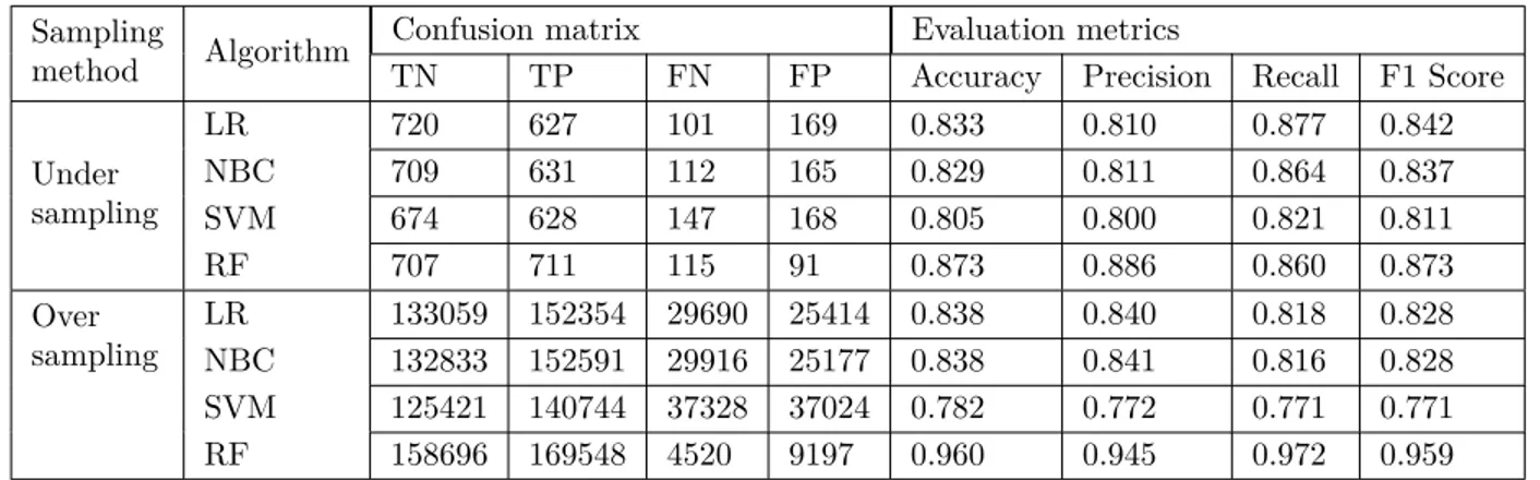
We first used a simple split of the data into training (70%) and test subsets. Table3 summarizes the results of the test data for all methods using the default parameters of the algorithms in their respective environment. In Table3, the first four rows correspond to undersampling results whereas the last four rows are for the results of the tests run on oversampled data. The first two columns show the sampling technique and the algorithms. The next four columns labeled as the confusion matrix show the raw counts of true negative (TN), true positive (TP), false negative (FN), and false positive (FP). The evaluation metrics are provided in the last four columns. We would like to note that no training data is used in the testing phase.
Table 3. Confusion matrix and evaluation metrics of test data - default parameters
Sampling
method Algorithm
Confusion matrix Evaluation metrics
TN TP FN FP Accuracy Precision Recall F1 Score
Under sampling LR 720 627 101 169 0.833 0.810 0.877 0.842 NBC 709 631 112 165 0.829 0.811 0.864 0.837 SVM 674 628 147 168 0.805 0.800 0.821 0.811 RF 707 711 115 91 0.873 0.886 0.860 0.873 Over sampling LR 133059 152354 29690 25414 0.838 0.840 0.818 0.828 NBC 132833 152591 29916 25177 0.838 0.841 0.816 0.828 SVM 125421 140744 37328 37024 0.782 0.772 0.771 0.771 RF 158696 169548 4520 9197 0.960 0.945 0.972 0.959
Observing Table3, we conclude that, logistic regression and Naive Bayes algorithms perform similar for all performance metrics, for both over- and undersampling. However, oversampling results are slightly better in terms of accuracy and precision and slightly worse for recall and F1-score. SVM is the worst performing
algorithm for this dataset for both over- and undersampling. Random forest model provides the best results in terms of accuracy, precision, and F1-score for both over- and undersampling. The recall value for undersampling is close to the others. The random forest algorithm run on the oversampled data provides the best results and the highest performance in all metrics.
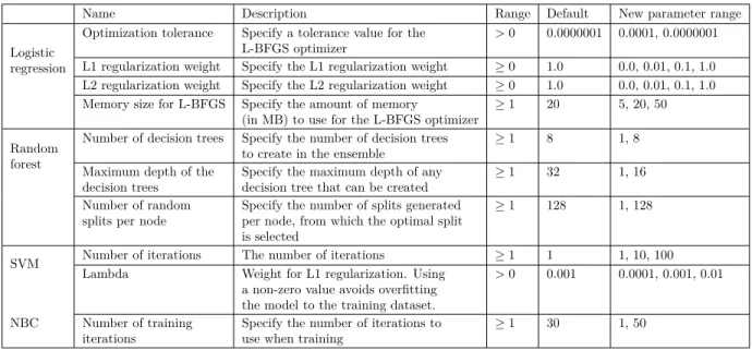
We also fine-tune all eight methods using the training set to squeeze out extra performance and improve the results. Algorithms calibrated via parameters fine-tuning which can change the outcome of the learning process. For each parameter combination in the fine-tuning procedure, we split the data into training (70%) and test subsets. We tuned all the models by searching for the best hyperparameters via grid search and kept the parameters with the highest F1-score on the test data. The hyper-parameters that are tested are presented in Table4.
Table 4. Grid search parameter range.
Name Description Range Default New parameter range
Logistic regression
Optimization tolerance Specify a tolerance value for the L-BFGS optimizer
> 0 0.0000001 0.0001, 0.0000001 L1 regularization weight Specify the L1 regularization weight ≥ 0 1.0 0.0, 0.01, 0.1, 1.0 L2 regularization weight Specify the L2 regularization weight ≥ 0 1.0 0.0, 0.01, 0.1, 1.0 Memory size for L-BFGS Specify the amount of memory
(in MB) to use for the L-BFGS optimizer ≥ 1
20 5, 20, 50 Random
forest
Number of decision trees Specify the number of decision trees
to create in the ensemble ≥ 1
8 1, 8
Maximum depth of the decision trees
Specify the maximum depth of any
decision tree that can be created ≥ 1
32 1, 16
Number of random splits per node
Specify the number of splits generated per node, from which the optimal split is selected
≥ 1 128 1, 128
SVM Number of iterations The number of iterations ≥ 1 1 1, 10, 100 Lambda Weight for L1 regularization. Using
a non-zero value avoids overfitting the model to the training dataset.
> 0 0.001 0.0001, 0.001, 0.01
NBC Number of training iterations
Specify the number of iterations to use when training
≥ 1 30 1, 50
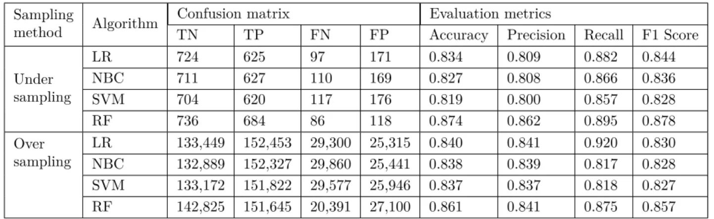
The results for fine-tuned algorithms are summarized in Table5. To avoid overfitting, no data in training set is included in the test set. We kept the hyperparameter setting which gives the best test results. The rows and columns of the table is the same as Table 3. On examining Table 5 and comparing with Table 3, we observe that the performance of the algorithms do not significantly improve for the undersampled data. The only recognizable change is on the recall metric for the random forest which has a mere increase from 0.860 to 0.895. For oversampling, we observe an increase for recall in logistics regression. Fine-tuning of the parameters improved the performance of the SVM algorithm in terms of all metrics. Interestingly, SVM is the only algorithm that benefited from fine-tuning in every metric for both over- and undersampled data. It is also worth noting that fine-tuning significantly decreased the performance of the random forest model in terms of all metrics. This suggests that random forest model is overfitting to the training data when fine-tuned.
Comparing Tables 3 and 5, we conclude that fine-tuning of the parameters does not increase the per-formance of the algorithms significantly without overfitting to the training data. In Table 6, we provide the averages of the evaluation metrics for 10-fold cross-validation results. Examining Table 6, we conclude that oversampling provides slightly better accuracy and precision (and slightly worse recall and F1-score) for LR, NBC, and SVM. On the other hand, RF with oversampling has significantly better performance than other algorithms in terms of all evaluation metrics.
Table 5. Confusion matrix and evaluation metrics of test data - tuned parameters.
Sampling
method Algorithm
Confusion matrix Evaluation metrics
TN TP FN FP Accuracy Precision Recall F1 Score
Under sampling LR 724 625 97 171 0.834 0.809 0.882 0.844 NBC 711 627 110 169 0.827 0.808 0.866 0.836 SVM 704 620 117 176 0.819 0.800 0.857 0.828 RF 736 684 86 118 0.874 0.862 0.895 0.878 Over sampling LR 133,449 152,453 29,300 25,315 0.840 0.841 0.920 0.830 NBC 132,889 152,327 29,860 25,441 0.838 0.839 0.817 0.828 SVM 133,172 151,822 29,577 25,946 0.837 0.837 0.818 0.827 RF 142,825 151,645 20,391 27,100 0.861 0.841 0.875 0.857
Table 6. Evaluation metrics of test data - 10 fold cross-validation.
Sampling method Algorithm Evaluation metrics
Accuracy Precision Recall F1 Score Under Sampling LR 0.829 0.809 0.860 0.834 NBC 0.822 0.804 0.854 0.828 SVM 0.803 0.787 0.832 0.808 RF 0.875 0.875 0.876 0.875 Over Sampling LR 0.838 0.839 0.818 0.828 NBC 0.836 0.837 0.817 0.827 SVM 0.828 0.824 0.813 0.818 RF 0.953 0.936 0.969 0.952
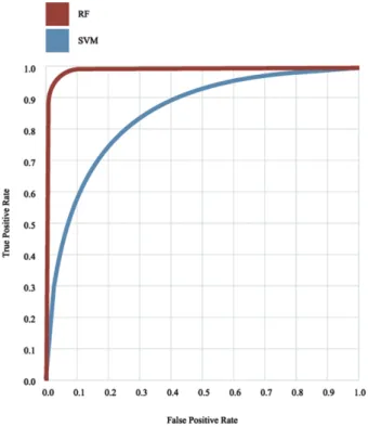
In the Figure, we provide the receiver operating characteristic (ROC) curve for the random forest and SVM methods applied to oversampled data. ROC presents a graphical representation of the trade-off between the percentage of true positives and false positives for every possible cut-off. The accuracy of the model is measured by the area under the ROC curve (AUC). The closer the AUC is to 1, the more accurate the model is. The random forest model has shown high level of accuracy with AUC = 0.992 and SVM model has AUC = 0.863.
4.1. Performance of oversampling on real data
Oversampling is a well-known way to deal with imbalanced datasets. However, generating exact duplicates or synthetic samples of the minority class may represent sampling from the actual distribution. When the oversampled data is used for both training and testing, results may be biased. In order to measure the effects of this bias, we tested all the algorithms on the original data. In other words, the training of the models are done on the oversampled data whereas the performance of the algorithms are calculated using the original data which represents the actual distribution more closely. The confusion matrix and the performance of the algorithms are shown in Table7.
Observing Table7 suggests high accuracy for all methods. However, precision and F1 scores are signifi-cantly lower than the previous runs tested on oversampled data. Recall that the dataset includes the loans that
Figure . Receiver operating characteristic curve - RF and SVM Table 7. Confusion matrix and evaluation metrics of test on original dataset.
Sampling
method Algorithm
Confusion matrix Evaluation metrics
TN TP FN FP Accuracy Precision Recall F1 Score
Oversampling
LR 507,497 1149 1549 85,206 0.854 0.013 0.426 0.026
NBC 508,463 1140 1558 84,240 0.856 0.013 0.423 0.026
SVM 468,950 1339 1359 123,753 0.790 0.011 0.496 0.021
RF 568,315 1328 1378 27,648 0.952 0.046 0.491 0.084
pass a filter designed by the bank and all of them are accepted. The main reason for low precision is that the actual minority class constitutes less than 0.5% of the dataset. The imbalance ratio is more than 220 for our dataset. In other words, for each data point in the minority class, there are 220 data points in the majority class. As the imbalance ratio increases, it is expected to have lower precision, recall, and F1 scores. When the imbalances are high, it is a good idea to compare the proposed methods to a case where the classification is done randomly, without using any information. The evaluation metrics can analytically be calculated for this no-information case. Consider the case where a no-information assignment is made: each data point is set to FPD with probability 0.5%. In this case it can easily be calculated that precision, recall, and F1-score on the minority class are equal to the proportion of instances that belong to the minority class. That is, random as-signment would result in less than 0.005 precision. The proposed RF model provides more than 10 times better precision, more than 107 times better recall, and more than 18 times better F1-scores than a no-information case.
To put a fair ground to discuss the performance of under- and oversampling approaches on top of avoiding effects of imbalanced data, we also tested our oversampling algorithms in a setting where there is an equivalent
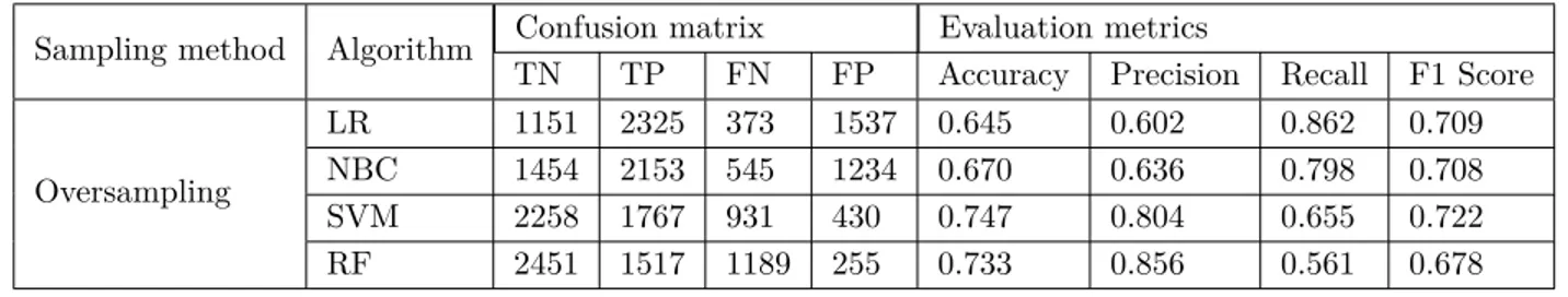
number of Class 1 and Class 0 (FPD and non-FPD) samples. In particular, we test all oversampling algorithms on the same test set in the undersampled data. The results for default and fine tuned parameter settings are provided in Tables8and9, respectively. Observing Table9, SVM and RF provide higher accuracy and precision whereas LR and NBC provide higher recall and F1-scores. When compared with Tables 3 and 5, we observe that all the performance for all evaluation metrics deteriorate. For example random forest model resulted in more than 96% accuracy with 94.5% precision in determining FPD loans when tested on oversampled data. However, when tested on the real and balanced dataset, the performance of the algorithm run on oversampled data deteriorates down to 73.3% accuracy with 85.6% precision. This may be due to the fact that generating synthetic data using SMOTE to balance an extremely imbalanced dataset may have harmed the training process of algorithms.
Table 8. Confusion matrix and evaluation metrics of test on original undersampled dataset-default parameters.
Sampling method Algorithm Confusion matrix Evaluation metrics
TN TP FN FP Accuracy Precision Recall F1 Score
Oversampling
LR 1480 2227 471 1208 0.688 0.648 0.825 0.726
NBC 1968 1731 967 720 0.687 0.706 0.642 0.672
SVM 2261 1603 1095 427 0.717 0.790 0.594 0.678
RF 2627 553 2153 79 0.588 0.875 0.204 0.331
Table 9. Confusion matrix and evaluation metrics of test on original undersampled dataset-tuned parameters.
Sampling method Algorithm Confusion matrix Evaluation metrics
TN TP FN FP Accuracy Precision Recall F1 Score
Oversampling LR 1151 2325 373 1537 0.645 0.602 0.862 0.709 NBC 1454 2153 545 1234 0.670 0.636 0.798 0.708 SVM 2258 1767 931 430 0.747 0.804 0.655 0.722 RF 2451 1517 1189 255 0.733 0.856 0.561 0.678 4.2. Feature analysis
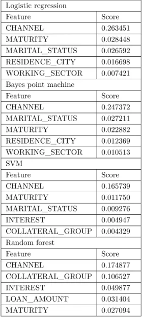
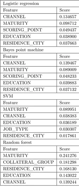
In general, 10-fold cross validated results suggest that the performances of the algorithms are satisfactory. In this section, we analyze the most important features in the study. In order to determine the most important features, permutation feature importance (PFI) is generated for all algorithms for both over- and undersampled data. The lists of the most important five features ordered by the importance scores are shown in Tables1and
2 in the Appendix.
PFI computes the importance scores for each of the feature variables of a dataset and helps to make sense of the features and its importance. We know that the classification is usually more responsive and sensitive to the changes in the important features. In our models, the channel for which the loan is given is found to be the most important feature with a nearly 20% of importance score. The importance of channel is consistent among all models.
In an attempt to understand that importance, we observe that being FPD is sensitive to the changes in channel. Hence, the value of the channel has a significant impact on predictions. The loans in this study can be allocated by two types of channels: 1) the bank itself (via bankers at the branch) and 2) business partners
of the bank (also referred to as the untied agents). We observe that the loans allocated by alternative channels are riskier or lack of control than the loans allocated by the branches. A two sample z-test indicated that the proportion of FPD loans allocated by the banks itself (0.0034) is statistically less than that allocated by the business partners (0.0049, P = 0.0000). Moreover, we conducted a two-sample t-test to check if the income levels of direct bank customers and customers applying at business partner are different or not. There is strong evidence that average reported income of direct bank customers is greater than customers applying for loans from business partners (P = 0.0000). We conclude that a more detailed analysis of individual partners and a reliable control mechanism for alternative channels is needed.
In models that are run on oversampled data, maturity date or the length of the loan is another important feature, showing itself in the top five important features in all methods. As the length of the loan decreases the probability that a loan goes FPD increases. It may seem interesting that the shorter loans have higher probability of being FPD. A loan with a shorter maturity date is a sign of a quick need for money and needs less planning in a highly volatile environment. On the other hand, longer loans need to be planned in detail, leading to smaller probability of being FPD. An interesting result is that the city of the customers presents itself to be an important feature. This can be due to the fact that a significant portion of the loans belongs to a major city.
5. Conclusions and future research directions
In this study, we provide a predictive analysis of the consumer behavior concerning a loan’s being FPD or not by using a real dataset of consumer loans with 598,669 records from a bank. We ran four classification algo-rithms using two resampling methods, leading to eight models. We provide the results for default parameters, tuned parameters, and 10-fold cross-validation results. We also calculated the performance of oversampling on real data. In order to get a fair comparison of over- and undersampling, we tested oversampling algorithms on undersampled data. All four algorithms provide at least 80% on all performance metrics when trained and tested on undersampled data. This suggests that all methods provide similar performances for undersampling. When the algorithms are trained and tested on oversampled data, all performance metrics improve. However, when tested on real and balanced dataset, the analysis show that the performance of all algorithms deteriorate. This may be due to the fact that generating synthetic data for an extremely imbalanced set (with a 20,000% percentage parameter) harms the training procedure of the algorithms. We conclude that for our extremely imbalanced dataset, synthetic data generation using the SMOTE procedure misguides the classification algo-rithms and results in lower performance for all metrics. In the literature there are many studies regarding the performance of oversampling highly imbalanced datasets (e.g., [16,17]). However, to the best of our knowledge, there are no studies that used the SMOTE algorithm with extreme oversampling percentages such as 20,000% like ours. A thorough analysis for the validation of SMOTE for extremely imbalanced datasets is proposed as future research.
All the models in this study can be used to predict whether the loan would be FPD or succeed in payment with a reasonable accuracy. It would benefit the bank before they make any decisions against these customers. The target is to minimize the risk of having a loan loss. In terms of finance, the classification models can help the bank prevent loan losses, improve the performance, and maximize the operational efficiency. From the banks’ point of view, it is not only important to determine whether a loan will be FPD or not, banks are also interested in when clients will not pay and a default will occur. Allocating loans to risky customers can be avoided by classifying and differentiating between the “good” and “bad” applications. Moreover, loans with higher probability of being FPD, should be monitored continuously.
Successful banks optimize lending by monitoring early warning signals closely. In general, banks utilize risk scorecards for their loan applicants and their repayment performances. Using the results of this study, bank managements may develop more reliable methods focusing on specific variables to evaluate the probability that a loan application would be FPD. This may lead to a situation where specific variables, weights, and cutoffs are assigned for different lending institutions, products, channels, and applicant segments.
Although this study yields significant results, it has some limitations. Notably, the use of only the accepted loan applications is an example. The study may be expanded by considering the rejected loans. That would help to obtain more persuasive results. Nevertheless, how to evaluate a rejected loan in terms of being FPD or not remains a question. More complex analysis can be performed using feature-selection techniques to assign weights on features by their importance in the future studies.
Acknowledgment
The authors would like to thank the anonymous reviewers for their constructive comments. References
[1] Thomas LC. A survey of credit and behavioural scoring: forecasting financial risk of lending to consumers. Int J Forecasting 2000; 2: 149-172.
[2] Menard SW. Applied Logistic Regression Analysis. 2nd ed. California, CA, USA: Sage Publications, 2002. [3] King G, Zeng L. Logistic Regression in Rare Events Data. New York, NY, USA: Academic Press, 2001.
[4] Khandani AE, Kim AJ, Lo AW. Consumer credit-risk models via machine-learning algorithms. J Bank & Fin 2010; 34: 2767-2787.
[5] Butaru F, Chen Q, Clark B, Das S, Lo AW, Siddique A. Risk and risk management in the credit card industry. J Bank & Fin 2016; 72: 218-239.
[6] Fitzpatrick T, Mues C. An empirical comparison of classification algorithms for mortgage default prediction: evidence from a distressed mortgage market. European J Operat Res 2016; 249: 427-439.
[7] Addo PM, Guegan D, Hassani, B. Credit risk analysis using machine and deep learning models. Risks 2018; 6: 38-57.
[8] Tang L, Cai F, Quayang Y. Applying a nonparametric random forest algorithm to assess the credit risk of the energy industry in China. Tech Forecasting & Soc Change ; In Press.
[9] Tsai MC, Lin SP, Cheng CC, Lin, YP. The consumer loan default predicting model–an application of dea–da and neural network. Expert Sys w Appl 2009; 36: 11682-11690.
[10] BRSA Turkish Banking Regulation and Supervision Agency. Turkish Banking Sector Main Indicators. Ankara, Turkey, 2017.
[11] Turkish Statistical Institute. Labor Force Statistics 2018. [12] Turkish Statistical Institute. Statistics Database.
[13] Bagherpour A. Predicting Mortgage Loan Default with Machine Learning Methods. Riverside, CA, USA: Academic Press, 2017.
[14] Shelke MMS, Deshmukh PR, Shandilya VK. A review on imbalanced data handling using undersampling and oversampling technique. Int J Recent Trends in Eng & Res 2017; 3: 444-449.
[15] Chawla NV, Bowyer KW, Hall LO, Kegelmeyer WP. Smote: Synthetic minority oversampling technique. J Art Int Res 2002; 16: 321-357.
[16] Luengo J, Fernández, A, García S, Herrera F. Addressing data complexity for imbalanced datasets: analysis of smote-based oversampling and evolutionary undersampling. Soft Computing 2011; 15: 1909-1936.
[17] Taft LM, Evans RS, Shyu CR, Egger MJ, Chawla N, Mitchell JA, Thornton SN, Bray B, Varner M. Countering imbalanced datasets to improve adverse drug event predictive models in labor and delivery. J of Bio Inf 2019; 42: 356-364.
Appendix
Table 1. Five most important features - undersampled models
Logistic regression Feature Score CHANNEL 0.263451 MATURITY 0.028448 MARITAL_STATUS 0.026592 RESIDENCE_CITY 0.016698 WORKING_SECTOR 0.007421
Bayes point machine
Feature Score CHANNEL 0.247372 MARITAL_STATUS 0.027211 MATURITY 0.022882 RESIDENCE_CITY 0.012369 WORKING_SECTOR 0.010513 SVM Feature Score CHANNEL 0.165739 MATURITY 0.011750 MARITAL_STATUS 0.009276 INTEREST 0.004947 COLLATERAL_GROUP 0.004329 Random forest Feature Score CHANNEL 0.174877 COLLATERAL_GROUP 0.106527 INTEREST 0.049877 LOAN_AMOUNT 0.031404 MATURITY 0.027094
Table 2. Five most important features - oversampled models. Logistic regression Feature Score CHANNEL 0.134657 MATURITY 0.098712 SCORING_POINT 0.049437 EDUCATION 0.038900 RESIDENCE_CITY 0.037663
Bayes point machine
Feature Score CHANNEL 0.139467 MATURITY 0.089009 SCORING_POINT 0.048233 EDUCATION 0.039883 RESIDENCE_CITY 0.037132 SVM Feature Score MATURITY 0.089951 CHANNEL 0.038383 EDUCATION 0.036189 JOB_TYPE 0.030307 RESIDENCE_CITY 0.017861 Random forest Feature Score MATURITY 0.241276 COLLATERAL_GROUP 0.181298 RESIDENCE_CITY 0.168130 EDUCATION 0.143022 CHANNEL 0.139244
![Highly luminescent CB[7]-based conjugated polyrotaxanes embedded into crystalline matrices](data:image/gif;base64,R0lGODlhAQABAIAAAP///wAAACH5BAEAAAAALAAAAAABAAEAAAICRAEAOw==)