YAŞAR UNIVERSITY
GRADUATE SCHOOL OF NATURAL AND APPLIED SCIENCES
MASTER THESIS
ON THE APPLICABILITY OF SIMULATION AS A
VERIFICATION TOOL FOR MARKOVIAN MODELS
OF PRODUCTION SYSTEMS
DENIZ DURMUŞ
THESIS ADVISOR: PROF. DR. SENCER YERALAN
DEPARTMENT OF INDUSTRIAL ENGINEERING
PRESENTATION DATE: 03.06.2016
ABSTRACT
ON THE APPLICABILITY OF SIMULATION AS A VERIFICATION TOOL FOR MARKOVIAN MODELS OF PRODUCTION SYSTEMS
DURMUŞ, Deniz
MSc, Department of Industrial Engineering Advisor: Prof. Dr. Sencer YERALAN
June 2016, 69 Pages
In the study of stochastic models of production and service systems, analytical results are quite often validated by simulation studies. This study calls into question the the ontological aspects, let alone the validity, of simulation. This thesis investigates the claim and its implications, and finally brings a resolution to the seemingly paradoxical practice, which has been entrenched in the dominant paradigms of operations research. In doing so, the thesis contributes to the state of the art by providing additional insights and a deeper understanding.
Key Words: Structure of Scientific Revolution, System's View, Paradoxes, Production and Service Systems, Simulation, Stochastic Models
ÖZET
BENZETİMİN ÜRETİM SİSTEMLERİNİN MARKOV MODELLERİNDE DOĞRULAMA YÖNTEMİ OLARAK UYGULANABİLİRLİĞİ
DURMUŞ, Deniz
Yüksek Lisans Tezi, Endüstri Mühendisliği Bölümü Danışman: Prof. Dr. Sencer YERALAN
Haziran 2016, 69 Sayfa
Üretim ve servis sistemlerinde kullanılan rassal modellerin analitik çözümleri genellikle benzetim çalışmalarıyla doğrulanmaktadır. Bu çalışma benzetimin ontolojik açıdan doğruluğunu sorgulamaktadır. Paradoksal görünümüne rağmen benzetimin neden ve hangi durumlarda başarılı olduğu ve hangi durumlarda da bir geçerleme yöntemi olarak yetersiz olduğu saptanmıştır.
Anahtar Kelimeler: Benzetim, Servis Sistemleri, Üretim Sistemleri, Rassal Modeller, Sistem Bakışı
ACKNOWLEDGEMENTS
“Once upon a time there was a young prince who believed in all things but three. He did not believe in Princesses, he did not believe in islands, he did not believe in God. His father, the king, told him that such things did not exist. As there were no princesses or islands in his father's domains, and no sign of God, the prince believed his father.
But then, one day, the prince ran away from his palace and came to the next land. There, to his astonishment, from every coast he saw islands, and on these islands, strange and troubling creatures whom he dared not name. As he was searching for a boat, a man in full evening dress approached him along the shore.
"Are those real islands?" asked the young prince.
"Of course they are real islands," said the man in evening dress. "And those strange and troubling creatures?"
"They are all genuine and authentic princesses." "Then God must also exist!" cried the prince.
"I am God," replied the man in evening dress, with a bow. The young prince returned home as quickly as he could. "So, you are back," said his father, the king.
"I have seen islands, I have seen princesses, I have seen God," said the prince reproachfully.
The king was unmoved.
"Neither real islands, nor real princesses, nor a real God exist." "I saw them!"
"Tell me how God was dressed." "God was in full evening dress."
"Were the sleeves of his coat rolled back?"
"That is the uniform of a magician. You have been deceived."
At this, the prince returned to the next land and went to the same shore, where once again he came upon the man in full evening dress.
"My father, the king, has told me who you are," said the prince indignantly. "You deceived me last time, but not again. Now I know that those are not real islands and real princesses, because you are a magician."
The man on the shore smiled.
"It is you who are deceived, my boy. In your father's kingdom, there are many islands and many princesses. But you are under your father's spell, so you cannot see them." The prince pensively returned home. When he saw his father, he looked him in the eye.
"Father, is it true that you are not a real king, but only a magician?" The king smiled and rolled back his sleeves.
"Yes, my son, I'm only a magician."
"Then the man on the other shore was God."
"The man on the other shore was another magician." "I must know the truth, the truth beyond magic." "There is no truth beyond magic," said the king.
The prince was full of sadness. He said, "I will kill myself."
The king by magic caused death to appear. Death stood in the door and beckoned to the prince. The prince shuddered. He remembered the beautiful but unreal islands and the unreal but beautiful princesses.
"Very well," he said, "I can bear it."
"You see, my son," said the king, "you, too, now begin to be a magician."”
TABLE OF CONTENTS ABSTRACT...iii ÖZET...iv ACKNOWLEDGEMENTS...v TEXT OF OATH...vii INDEX OF FIGURES...x INDEX OF TABLES...xi INDEX OF SYMBOLS...xii
CHAPTER ONE THE SCOPE AND CONTRIBUTION OF THE THESIS...1
CHAPTER TWO INTRODUCTION...3
2.1. THE STRUCTURE OF SCIENTIFIC REVOLUTIONS...4
2.2. CRITICAL THINKING AND ITS CONTEXTUAL RELATIONSHIP WITH PARADOXES...7 2.3. PARADOXES...8 2.3.1. VERIDICAL PARADOXES...8 2.3.2. FALSIDICAL PARADOXES...9 2.3.3. ANTINOMIES...10 2.4. PRODUCTION LINES...11
CHAPTER THREE SIMULATION OF PRODUCTION AND SERVICE SYSTEMS...13
3.1. THE PARADOX...13
3.2. THE M/M/1 QUEUE...13
3.3. OBSERVATIONS AND CONCLUSIONS...18
CHAPTER FOUR MARKOVIAN MODELS OF PRODUCTION LINES...21
4.1. A THREE STATION LINE WITH NO BUFFERS...22
4.2. A TRUNCATED MODEL OF THE THREE STATION PRODUCTION LINE WITH NO BUFFERS...24
4.3. MORE ACCURATE TRUNCATED MODELS OF PRODUCTION LINES WITH NO
BUFFERS...27
CHAPTER FIVE CONCLUSIONS AND FUTURE RESEARCH...31
REFERENCES...33
APPENDIX 1 – CRITICAL THINKING...37
APPENDIX 2 – M/M/1 SIMULATION IN SCILAB...41
APPENDIX 3 – THE MAXIMUM LENGTH OF THE M/M/1 QUEUE...43
APPENDIX 4 – THE ALGORITHM...49
INDEX OF FIGURES
Figure 1. Revolution In Science...5
Figure 2. Simulation Run Results...15
Figure 3. The Average Number Of Customers In The System As A Function Of The Simulation Runtime...15
Figure 4. Server Utilization As A Function Of The Simulation Runtime...16
Figure 5. Nmax As A Function Of Runtime, As Obtained By Simulation...17
Figure 6. Nmax As A Function Of Runtime, As Computed Theoretically...18
Figure 7. Production Rate As A Function Of Breakdown And Repair Probabilities...23
Figure 8. The State Transition Diagram Of The Truncated Bufferless Three Station Model..26
Figure 9. Absolute Percentage Errors As Functions Of Model Parameters...27
Figure 10. A Section Of Ascending And Descending By Escher...39
Figure 11. The Probability Distribution Function Of Nmax (l9, M10, T=1000)...45
Figure 12. The Probability Mass Function Of Nmax (=9, =10, T=1000)...45
Figure 13. A Portion Of The Output Of PLT...53
Figure 14. The Rudimentary Command-Line Help Listing Of SXB0T...55
Figure 15. Executing SXB0T...55
INDEX OF TABLES
Table 1. System States Of The Production Line...22
Table 2. Steady-State Probabilities Of The Production Line Model (q=0.01, R=0.1)...24
Table 3. States With Fewer Than Two Stations Under Repair...25
Table 4. Number Of System States (N/K Models, N Stations, At Most K Down)...28
Table 5. Average Percentage Error Of The N/1 Truncated Models...29
INDEX OF SYMBOLS N Number of stations of the production line.
D Maximum number stations allowed to be down at any given time. q Breakdown probability.
r Repair probability.
U Station state “Up and operating”. D Station state “Down and under repair”.
B Station state “Blocked (operational but unable to unload the finished part)”. S Station state “Starved (operational but waiting for a part)”.
X Station state “Down and blocked (down, under repair but unable to unload the finished part)”.
1 CHAPTER ONE
THE SCOPE AND CONTRIBUTION OF THE THESIS
We take a rather phenomenological approach to reviewing the various stochastic models developed within the operations research community over the past half century. We attempt to distance ourselves from the customary set of assumptions and hitherto discipline-customary simplifications.
Although the thesis is composed with the engineer community in mind, it is presented in a format suitable for the non-engineer reader. In particular, we discuss the fundamental ideas and their logical implications in the body of the thesis, while computational and analytical details are relegated to the appendices. Moreover, a rather extensive review of the basic concepts appears in the various sections and in the literature review. Readers familiar with these supporting fields may freely skip the literature review.
In this treatise, we examine aspects of stochastic models in production and service systems. We dwell on the meaning and essence of simulation studies which ubiquitously accompany most of the published research. Simulation is most often employed as a verification tool, and occasionally as an investigative tool. We question the ontological aspects of state-space-based stochastic models (e.g. Markovian models) and investigate if simulation rises up to the stature of being a determinant of verification.
Specifically, we address the following conundrum. It is observed that Markovian models give rise to inordinately large state spaces. Production line models may easily have state spaces with cardinalities in the order of 10100 or more. How is it then, that simulation is a justifiable validation tool, when it is obvious that a regular simulation run may never visit all of the states of the Markovian model?
This conundrum is very seldom address in the literature. Moreover, as simulation constitutes a fundamental component of the dominant paradigm, it behooves us to
scrutinize its role and its limitations. This will not constitute extraordinary science, but will serve to question the dominant paradigm, and hopefully lead to either the reinforcement or the degradation of the dominant paradigm. Either way, we submit that it is valuable research, albeit not in the form of normal science.
The paradox is addressed and resolved. The resolution not only provides insights into the use of simulation as a verification tool, but also presents facilities to develop novel approximations to the traditional Markovian models. The contribution of this is thesis should be considered mainly as a study to provide deeper insights and a better understanding of the use of various analytical and conceptual tools and techniques. As a direct corollary, we are able to identify when simulation becomes a valid tool and when it does not. Thus, the study sheds light onto the current practices by alerting the practitioner when not to rely on simulation as a tool of verification. It should be noted that, by its nature, the topic required dealing with larger sets of data, whose exact solutions are needed for the conceptual analysis. Accordingly, much effort was involved in code development. In particular, it is noteworthy that some source code are in the order of 1 gigabyte. Clearly, a gigabyte of code is not to be written manually. The approach here was to write code that in turn generates source code, later to be incorporated into downstream compiling and linking. The code development itself may also be considered as a contribution, as it provides a template or framework to the generation of multi-echelon software.
The following sections give a brief background in the structure of scientific revolutions critical thinking, paradoxes and production lines. Afterwards, we will revisit our conundrum and define it more precisely.
2 CHAPTER TWO INTRODUCTION
This thesis strives to investigate fundamental properties of a class of models commonly used in industrial engineering. Unlike most works that develop extensions to known models, approaches, or techniques, the emphasis here is to gain insights and understanding. As a direct consequence of our desiderata, much investigative work was needed before finally developing the ideas presented here. Clearly, seeking novelty, by definition, requires that we disengage from the dominant tools and techniques prescribed for a given subject area. This work, accordingly, required a considerable amount of self learning in related areas such as the nature of scientific paradigms, chaos theory, modeling competitiveness in multi-predator multi-prey models, industrial dynamics, general systems theory, and complexity.
The specific area of research is Markovian models of production and service systems. Although the area of stochastic models of production and service systems is quite broad, a specific focus area, namely that of production lines, is sufficient to illustrate the ideas. Again, our emphasis is not in the extension of existing models, but in obtaining further insights into, and a deeper understanding of, these models. We made every effort to keep the examples simple so that the reader is not prevented from seeing the proverbial forest for the trees. Accordingly, we pick discrete Markovian models of multi-station production lines with no inter-station buffers. Some aspects of the work require the use of analytical comparisons. We chose the simplest queueing model, namely the M/M/1 queue for this purpose. Once again, our work also relates to the use of simulation as a tool. Here, we wrote the simulation code in the general engineering computational environment of Scilab.
The computational aspects of our work are also somewhat unusual. Most of the developed code does not compute, but rather, generate source code for downstream compiling and execution. In this sense, it is closer to hard AI (artificial intelligence)
than it is to computation. It thus follows that we are not much interested in computation times, other than the practicality of waiting for the code to be so generated. All code development was done in source environments using open-source tools. Detailed information about the code is given in the appendices.
2.1. THE STRUCTURE OF SCIENTIFIC REVOLUTIONS
It is already stated that the current work aims to develop insights and understanding, rather than to pursue extensions within the framework of a dominant set of tools and techniques. Such tools and techniques are called a “paradigm”. The word “paradigm” was not a popular until it was used by Thomas Kuhn (1970). Kuhn, the physicists and philosopher, introduces this notion in his 1965 book “The Structure of Scientific Revolution”. Kuhn introduces the phenomenon of a “Paradigm Shift” to emphasize the distinction between what he calls “Normal Science” and “Extra-Ordinary Science”. Before explaining normal and extra-ordinary sciences, let us first dwell further on what a paradigm is.
The word “paradigm” comes from the Greek word “paradiegma”, which means “example”. It is used as a guide for a better understanding of a phenomenon. On the other hand, in its contemporary use, the word “paradigm” is mostly used to describe the entire whole of a technique or a value in a community. Remarkably, the word “paradigm” is one of the few words that have both monolithic and holistic notation. This observation may not be adequate in rigorous philosophical context. However, in this thesis, any differentiation of the concept of paradigm, between these two implications is not necessary.
We can basically summarize Kuhn's ideas of a scientific revolution in three stages, as seen in the figure below.
In pre-paradigmatic stage, there are a few ideas that compete with each other, and try to become a dominant (or alpha) idea. This is then labeled the alpha-paradigm. We may call this stage, the competition of paradigms in which the scientists are clustered behind their favorite paradigm, as the process tries to pick one of the paradigms. After some time, most of the proposed paradigms are eliminated from further consideration, and just a few of them are left. At the end of this stage, one paradigm becomes the alpha-paradigm. This represents the conviction of a majority of the scientists that following the chosen alpha paradigm to be more appropriate and effective for the development of the field. After the competition ends, and one paradigm becomes the winner, science is conducted through “normal (ordinary) science”.
In normal science, the scientists operate within the guidelines of the winning paradigm, find its limits and try to extend its potential. As time passes, and even though the community has some problems with the dominant paradigm, trust of, and a familiarity to the dominant paradigm develops over the years. Often, the community is blinded and does not accept the paradigm's shortcomings, or is afraid of what might happen after letting go of the dominant paradigm. This is called “Paradigm Paralysis”. It is very hard at this point to accept that the existing
paradigm is not adequate, to break the chains for a new paradigm, and make a leap. But eventually the paradigm causes a crisis in the scientific community, and this leads us to the next phase of the science, that is, what Kuhn names “Extraordinary Science”.
At this stage, to answer all those unanswered questions, a scientific revolution is needed. Creating a new paradigm, a methodology, requires more work and patience compared to normal science. Kuhn's idea of a revolution in science has significant philosophical ramifications. From the beginning of the 20th century, the beginning of the logical positivism, it was well accepted that science is a cumulative progress. But according to Kuhn, science is not cumulative, and we need to make a leap to make a progress. A crucial fact of extraordinary science, according to Kuhn, is that different scientific paradigms are incommensurable. If two scientists from different paradigms try to find a new method on the same subject, they cannot compare their work to each other. Their experiments and observations depend on the observer, thus one's work may seem irrational or irrelevant to the other one. In this stage, new proposed methodologies are conducted and proposed to the community and we get back into the pre-paradigmatic stage.
We cannot say whether ordinary or extra-ordinary sciences is better. Because these two phenomena are interconnected. They are co-dependent in a cyclical self-triggering fashion. Only together as a whole, one can speak of science. But the question is, since science depends on the paradigm of the experimenter or observer, is progress in science is arbitrary?
It was stated that this thesis aims to develop understanding and insights. Actually, it might be more appropriate to say that we wish to work on something other than normal science. The pursuit of extraordinary science, by definition, is not possible by a checklist or through an established technique. For this would mean there is already a paradigm to conduct extraordinary science, which logically is a contradiction. As an alternative to extraordinary science, however, academic research may be oriented to investigate and question the dominant paradigms. The hope is that such investigation may lead to extraordinary science, or at least bring about deeper understanding, either reinforcing or eroding the dominant paradigm. Parenthetically, let us also divulge why we want to work outside the dominant paradigm. The survey of the greater
literature in philosophy of engineering, philosophy of science leads to the question of the role of an engineer in academia (Engineering, 2010). A case in point, if the role of an engineer is to apply science, why is so much academic engineering research oriented towards basic research, arguably void of any hope for application or implementation? There are numerous articles that claim that studies in academia are irrelevant to the extent that they cannot be applied in real world (Anonymous Academic, 2014; Panda and Gupta, 2014; Boehm, 1980; Economist, 2010 ; Jon Excell, 2013).
We have to state that this study is not exactly Extraordinary Science. However, we do not have any references to create a checklist to get results. This study focuses on the simulation in production lines and queues. Literature review on production lines and paradoxes are given as a subsection in Chapter 1. The scope of the thesis is explained in Chapter 2. Analysis in M/M/1 Queue and Production Line are given in Chapter 3, and Chapter 4, respectively. Lastly, Conclusion and Future Studies is given in Chapter 5.
2.2. CRITICAL THINKING AND ITS CONTEXTUAL RELATIONSHIP WITH PARADOXES
Science and technology are what they are now due to the scientists and academicians, who have been skeptical within a rigorous framework of critical thinking. Costa (1985) gathered different definitions of critical thinking from different works. Critical thinking might be defined as thinking which achieves a rational conclusion using adequate information by analyzing, observation, evaluation, or explanation. The Critical Thinking Community (Critical Thinking Community, n.d.) also has a definition which is widely accepted. They define critical thinking to be “the intellectually disciplined process of actively and skillfully conceptualizing, applying, analyzing, synthesizing, or evaluating information gathered from, or generated by, observation, experience, reflection, reasoning, or communication, as a guide to belief and action” (Critical Thinking Community, n.d.).
According to Paul (1991), there are three groups of mental structures to be considered as an open-minded thinker. The first one is micro-level skills by which one distinguishes a subsentence, a skeptical assumption, or inconsistency. At the
macro-level, there are skills by which one makes contributions to discussions, creates theories, and knows how to approach a subject critically. The third group of essential skills to critical thinking contains the aspects of mind such as intellectual virtues and moral commitments. Paul (1991) also gives a detailed table of the elements of critical thinking.
Further examples of critical thinking are given in Appendix 1.
2.3. PARADOXES
The word of “paradox” stems from Greek word “parádoxos” which its root based on “pará” (“beyond”) and “dóxa” (“expectation”) means contrary to expectation. Felkins (1995) states that the paradoxes may occur from our lack of understanding which may caused by the inadequacies of our language. In most of the paradoxes, the conclusion is seemingly both true and false at the same time, and thus present unresolved contradictions. Since the paradoxes show us the flaws in our understanding and the way we think, contradiction is essential to paradoxes.
Paradoxes are also self-referenced and sometimes they include circularity. One of the most known paradox, “This sentence is a lie” is self-referenced. “A goes to B”, “B goes to A” are the basic circular paradoxes. However, paradoxes may caused by false or prejudiced statements which may be come from generalizations.
Cantini (2007) wrote in detail the development of paradoxes and contemporary logic. Cucić (2009) also wrote the development of paradoxes and very well gathered notable classifications made by other researchers.
There are several types of paradoxes. The classification of paradoxes by Quine (1966) might be reckoned as a basis for other classifications. According to Quine, there are three types of paradoxes as described in the following sections.
2.3.1. VERIDICAL PARADOXES
Veridical paradoxes are also known as Truth-Telling or Verification paradoxes. They lead us to a seemingly absurd conclusion, however when a new premise is included, it convinces us that the conclusion is valid. This type of paradoxes may occur in situations where the language we use, or our understanding thereof, is not adequately
sufficient for the circumstances. We may need more information or a new point of view on these paradoxes. Quine gave these examples to explain veridical paradoxes: The Frederic Paradox: In the opera named Pirates of Penzance, the character Frederic who works as an apprentice for the pirates, wants to leave because he wants to fell in love poetically. His friends in the ship fell badly about it, and do not want him to leave. On his 21st birthday, they tell him that he cannot leave the ship because in his contract, it is specified that he may leave at the age of 21, but he is currently only 5 years old, and that he has to remain with the pirates for 63 years. Even though it seems absurd at first, we can easily solve the paradox by saying that he was born in the leap year.
The Barber Paradox: Another example for veridical paradoxes that Quine gives is the so-called Barber Paradox. Here, there is a village barber who shaves all and only the men who cannot shave themselves. The first question comes to mind is that who shaves the barber. If the barber cannot shave himself, then the barber has to be shave himself. But, if he can, then he should not. There is an obvious circularity in this paradox. However, as stated earlier, such paradoxes can be viewed as an indication of our lack of understanding, or as inadequacies of our language. Thus, Quine's resolution of Barber Paradox might be the easy way out. After all, it is not stated if there is any other barber. If there is another barber in the village, then the second barber can shave our hero, thus the paradox unravels. But if there is no other barber in the village, we have no argument that only barbers can shave other men. By this we can conclude that arguments that create paradoxes might narrow our viewpoint.
2.3.2. FALSIDICAL PARADOXES
Falsidical paradoxes are the ones that not only seem false, but are false. The conclusions established from the falsidical paradoxes are evidently absurd, but the arguments creating the paradoxes seem true. The causes that create the falsidical paradoxes are the hidden fallacies in the arguments. Most common falsidical paradoxes are the mis-proofs of algebra.
The 2=1 proof by Augustus De Morgan: Assume that X=1. If we multiply each side of the equation by X, we obtain X2 = X. Then we subtract 1 from each side, we get, X2-1 = X-1. We extend the left side of the equation as, (X-1)(X+1) = X-1. If we
simplify the equation by dividing each side by (X-1), we obtain, X+1 = 1. Since X=1, we get, 2 = 1. The conclusion is obviously wrong, even though we applied reasonable steps on the equation. However, what is not noticed is, X-1=0. Thus the fallacy in the argument is dividing the equation by X-1.
Achilles and the Tortoise: Another example that Quine gives is one of the Zeno Paradoxes, Achilles and the tortoise. As Silagadze writes (2005), Zeno claims that plurality, motion, and change are illusions, and established paradoxes categorized by these concepts. Achilles and the tortoise is one of the three paradoxes to defy that the motion is real. In this paradox, Achilles and the tortoise decides to make a footrace. Since the tortoise is really slow, Achilles gives him a head start. The paradox establishes a conclusion at this point, that the fast runner can never overtake the slow runner. Zeno says that where the fast runner gets after an interval of time, the slow runner will be further from that point. Thus the motion is just an illusion. However, what Zeno does not see is that Achilles will overtake the tortoise either in an infinite or a finite time. The resolution of this paradox and other Zeno Paradoxes are given by several works (Silagadze, 2005; Dowden, n.d.; Byrd, 2010).
2.3.3. ANTINOMIES
Antinomies are the paradoxes that do not fit in these two categories above. They create a “crisis in thought” as Quine states (Quine, 1966). If one cannot find a fallacy in an argument, or cannot be convinced by the conclusion of the paradox, then these are called antinomies. The following examples are generally accepted as antinomies. Grelling – Nelson Paradox: Before explaining the Grelling – Nelson Paradox (a.k.a. Grelling's Paradox), let us first define the adjectives “homological” and “heterological”. Homological is defined as “describing itself”. “English” is a homological word, since the word itself is English. “Word” is also homological, since the “word” is also a word. Heterological, on the other hand, is defined as “not describing itself”. “German” is a heterological word because it is not a German word. Long is also a heterological one since “long” it is not a long word, but a short, monosyllabic word.
What is paradoxical here is whether the word “heterological” is heterological or homological. The definition of heterological is “not describing itself”. Thus the word
“heterological” should not describe itself. But it does, as all words have a meaning. Thus, we conclude that the word “heterological” is homological. However, if it is a homological word, heterological defines itself, and thus is a homological word. Thus there is a contradiction due to self-reference.
The Paradox of Epimenides: This paradox is very similar to Grelling's paradox. Epimenides was a Cretan who said “All Cretans are liars”. This is also a self-referencing paradox, which has the same structure as “This sentence is a lie”. If all Cretans really are liars, then the sentence of Epimenides is true. Therefore, he told the truth where the contradiction causes a paradox.
If we consider that some aspects of nature cannot be explained in any circumstance, antinomies are reasonable explanations of paradoxes. However, if we are pioneers in supporting that nature itself can always be explained but today's knowledge and experience are insufficient to explain, we can say that antimonies are also the paradoxes that would be resolved if more information were provided. Thus antinomies can also be considered as veridical or falsidical paradoxes. Furthermore, Quine (1966) states that “One man’s antinomy can be another man’s veridical paradox, and one man’s veridical paradox can be another man’s platitude”, meaning that defining the type of paradoxes is relative upon one's knowledge and experience.
2.4. PRODUCTION LINES
Production lines are linear arrangements of workstations, where workstations display some type of randomness. Typically, the randomness may be due to random service times, or due to station breakdown. Often interstation buffers are employed to compensate for these sources of randomness. This makes the subsystem of each station with its preceding buffer look like a simple queueing system. Thus, production lines may also be regarded as tandem queues. This invites the generalization of tandem queues to queueing networks.
Production lines have received much attention in the industrial engineering and operations research literature. Starting from the mid-fifties, considerable work has been done in both understanding the fundamental mathematical structure of queueing networks, and in developing computational techniques to predict the performance of
production lines. The latter concern underlies the justification of much of the simulation tools developed in the dawn of the computer age.
Analytical models for multi-station production lines, which are the focus of this research, are classified in two main categories. These categories depend on whether time is considered to be continuous or discrete. Discrete models are more suitable for paced assembly lines, often seen in automotive production. Modeling these systems is often done by continuous- time and discrete-time Markov models. Continuous-time models are favored in the process industry where no identification of the individual units exists, (e.g. chemical industries). In almost all cases, focus is on the evaluation of two primary performance measures: the production rate, and the expected number of items in the buffers.
The studies of Schick and Gershwin (1978), Muth (1979), Muth and Yeralan (1981), and Gershwin and Schick (1983) are early examples of discrete -time Markovian models. Studies conducted by Yeralan et al. (1986), Yeralan and Tan (1997) provide examples of continuous-time models.
There are many extensions to these basic models. For instance, Maggio et al. (Maggio, Matta, Gershwin, and Tolio, 2009) present closed-loop systems. These may be considered as queueing networks. Such closed-loop systems are seen in industries where hot pallets are used to hold the workpiece while it progresses through the manufacturing system. Once the workpiece is completed, the hot pallets are returned to the beginning of the line. Thus, the models track the hot pallet.
There are several textbooks on the subject, to which the reader is referred for detailed information (Altiok, 1996; Askin and Standridge, 1993; Buzacott and Shanthikumar, 1993; S.B. Gershwin, 1994; Li and Meerkov, 2009; Papadopolous, Heavey, and Browne, 1993; Tempelmeier and Kuhn, 1993).
3 CHAPTER THREE
SIMULATION OF PRODUCTION AND SERVICE SYSTEMS
It is customary among those studies reported in the literature of stochastic models of production and service systems to find simulation runs that accompany any given analytical development. Simulation is most often used as a tool of verification. We do not question the basic premise that simulation may be used in this capacity. However, many models are developed in a brute force manner that the meaning of the very premise of a model becomes vulnerable to criticism. A recent report by Yeralan and Büyükdağlı (2015) mentions an automotive plant with 168 robotic workstations arranged in a serial manner. Even without inter-station buffers, given that each workstation is subject to breakdown, the system modeled as a time discrete-space Markov chain has over 1050 states. If we were to visit a different state every nanosecond, a complete tour of all the states would take 1027 times the age of the universe. This is an incomprehensible number – so incomprehensible that Yeralan and Büyükdağlı calls into question the ontology of such a model.
3.1. THE PARADOX
We routinely see simulation models developed and used to analyze stochastic Markovian models of production and service systems. Given that there are an inordinate number of system states in typical Markovian models, how is it the case that simulation gives us answers which would take total enumeration a practically endless amount of time? We attempt to address and answer that very question in this thesis.
3.2. THE M/M/1 QUEUE
First, consider a system modeled as a continuous-time, discrete-state Markov process. We pick a system with the number of states even greater than the 1050 mentioned for the automotive plant model. The continuous-time M/M/1 queue has a
single server and an input queue. Customer arrive to the system with a rate of . Similarly, the service of a customer, provided that the system is not empty (and hence the server is not idle), is completed with rate . The number of customers in the system uniquely determines the state of the system. It is clear that the number of customers in the system is unbounded. Thus, the system state space is unbounded, with an infinite number of elements. A complete tour of all the states of the system is, by definition, impossible in a finite amount of time, irrespective of how quickly we visit each state.
In analyzing the M/M/1 queue, we often investigate two performance measures: the expected number of customers in the system, and the utilization of the server. The latter refers to the probability that the server is busy servicing a customer, or equivalently, that the system is not empty.
It is a relatively pedantic task to show that the system is stable if the arrival rate is less than the service rate . Or the ratio =/, which is also referred to in the discipline as the traffic intensity, is less than unity. If the traffic intensity is greater than unity, then the system becomes unstable and the number of customers in the queue is expected to keep growing over time, never converging to a finite value. Analytical work quickly reveals that if the traffic intensity is less than unity, then the expected number of customers in the system is 1/(1-). Similarly, the server is busy with probability and idle with probability (1-) (Hillier and Lieberman, 2009). We next build a simple simulation model for this infinite-state Markov process (see Appendix 2). A typical result from the simulation runs is given below.
simulation parameters
---Run time: 1000 Arrival rate: 9.00 Service rate: 10.00 Number of arrivals: 9023 simulated performance measures ---Utilization: 0.89 Average number of customers: 7.76 Maximum number of customers: 54 computed performance measures ---traffic_intensity: 0.90 ave_num_in_system: 9.00
Figure 2. Simulation Run Results.
As seen, with a traffic intensity of 0.9, with a total of about 9000 transactions (9023 customers arriving), we obtain fairly good estimates for the performance measures. The utilization is found to be 0.89 (0.90 theoretical), and the average number of customers in the system was found to be 7.76 (theoretical 9.00).
Increasing the run time, and hence the number of transitions gives results even closer to the theoretical values. The graphs below show how the estimated performance measures are affected by the runtime.
Figure 3. The Average Number of Customers in the System as a Function of the Simulation Runtime.
Now, the question remains, as to how is it possible for a simulation run of only a few thousand transaction to yield performance measures so close to the theoretical values (relative errors in the range of a few percent), given that a total enumeration of the states is impossible. After all, the M/M/1 queue has an infinite number of states. Since we run the simulation for a limited number of transactions (a limited amount of simulated time), it is clear that the simulation does not visit all possible states. We next inquire how many distinct states the simulation run actually visits.
Clearly, the M/M/1 queue may only make a transition to an adjacent state. That is, if there are N>0 customers in the system, the next transition would be to either state N+1 or to state N-1. Hence, the number of customers in the system throughout the simulation run is bounded by a maximum and minimum. It is customary to start the system at state 0 (empty system). Then the maximum number of customers in the system, Nmax, during the simulation run is a finite number. Again, it is quite clear that Nmax is a function of the simulation run. As the simulation run time increases, we may expect Nmax to also grow, as there is more time for visiting states with a higher number of customers.
We modify the simulation code given in Appendix 2 and keep track of Nmax. It is then plotted as a function of the runtime.
Figure 4. Server Utilization as a Function of the Simulation Runtime.
Figure 5 shows the results of the simulation runs. Each simulation run has a service rate of 10, and a runtime between 100 and 5000 time units. Five different arrival rates are used: 1, 3, 5, 7, and 9. The simulation was run and the maximum number of customers in the system (Nmax) throughout the runs were recorded. Each point on the graph is actually an average of 50 runs with identical parameters. It is interesting to observe that, in each case, Nmax quickly and asymptotically approaches a constant long-term value.
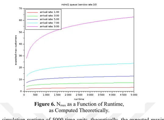
It is possible to analytically compute the expected value of Nmax as a function of the system parameters and the length of time the system is observed. Such computation falls into the domain of transient analysis. Appendix 3 gives the transient analysis for an M/M/1 queue which starts with an idle server and runs for a given period of time. The analytical work shows how Nmax may be computed. Here we will suffice with simply graphing the theoretical values of Nmax and comparing them to the figure above.
Figure 5. Nmax as a Function of Runtime, as Obtained by Simulation.
With a simulation runtime of 5000 time units, theoretically, the expected maximum number of customers in the system is about 65.
3.3. OBSERVATIONS AND CONCLUSIONS
In effect, the simulation runs successfully evaluates the two performance measures, the utilization probability and the expected number of customers in the system, by only visiting a handful (say 100) of states out of the possible infinite number of states. The implications of this observation are quite significant in many ways.
First, it shows that the value of simulation as an investigative tool is not only in its utility to collect data and obtain statistics, but also in delineating and concentrating on the more likely states and ignoring (completely) the states which have negligible effect on the performance measures. In effect, the simulation only considers a “truncated” system, where among the infinite number of states, only a few hundred states are dealt with. In other words, if we were to build a simulation model of the M/M/1 queue and another for a modified M/M/1 queue where arrivals to the system with 100 customers in it were lost, the two models would give us exactly identical numerical results.
In a related observation, we see that simulation initial conditions are of importance. For example, if we were to start the given M/M/1 queue simulation with 1,000,000
Figure 6. Nmax as a Function of Runtime, as Computed Theoretically.
customers in the system and ran it for a few thousand time units, we would always get the utilization to be 100%, since the simulation run would not be long enough for the system to reach a steady-state.
A similar case could be made for different performance measures. Suppose the probability that there are 1000 customers or more in the system is taken as a performance measure. For the system discussed above, our simulation runs would always return this value to be zero, since there will never be enough time for the runs to observe such states with 1000 or more customers. Theoretically, however, these performance measures are available quite easily.
Finally, and perhaps most importantly, the observations in this chapter point to some insights concerning the modeling of production and service systems. As discussed, realistic applications lead to unimaginably large state spaces. Brute force computing the steady-state probabilities, as it is customarily pursued in the literature, is perhaps rather superfluous. Inspired by the discussions above, one may attempt to build a “truncated” model of the system and solve it. Of the 168 stations of the automotive line, how many of the stations could be down at any given time? Clearly, the state where all 168 stations are down is very very unlikely. If the probability of breaking down is in the range [0, 0.01], then in the worst case, the probability that all 168 stations break down is about 10-336. Granted there are more ways to enter the state where all 168 stations are down, but still, the argument is quite strong that the state with all 168 stations down will never be observed.
4 CHAPTER FOUR
MARKOVIAN MODELS OF PRODUCTION LINES
The preceding chapter provides insights into simulation as a modeling and computational tool. In particular, we find simulation to be useful in cases where the performance measures sought are, in some particular sense, commensurate with the general nature of simulation. It is clear that simulation is not a substitute for exact models, e.g. computing the steady-state probabilities of a Markovian model, when unusual performance measures are of interest.
In this chapter, we incorporate the insights gained into models of production lines. We aim to address and resolve the claim (see Yeralan and Büyükdağlı, 2015) concerning the validity – in fact, the ontological standing – of Markovian production line models when the state space is simply telescoped by considering successive Cartesian products of the station states. Consider that, when there are about 100 stations, each station being in a state down or up, we have at least 2100 system states. This is an unfathomably large number. No current simulation study can be expected to visit all of these states. However, we see from inspecting the M/M/1 queue that not all states need to be considered when seeking the usual performance measures. In particular, almost all studies start with an investigation into the production rate of the line. The question is, parallel to the insights regarding the M/M/1 queue, is it reasonable to consider a truncated state space of the production line and obtain a good estimate to the production rate. After all, simulation is not expected to visit all such states, while its results are considered to constitute a benchmark. In order to address this question, we consider a minimalistic line, as we are interested in the fundamentals rather than any of the details. The investigation is constructed in the next section.
4.1. A THREE STATION LINE WITH NO BUFFERS
Consider a three-station production line with no buffers. The line is assumed to operate in discrete time, as explained in (ref MY81). There are five station states: up and operating (U), up but blocked (B), up but starved (S), down and under repair (D), down, blocked and under repair (X). With three stations and no buffers, the Markov chain has 32 states. These states are listed below.
Table 1. System States of the Production Line. Index Station States Index Station States Index Station States Index Station States 0 DDD 8 DSS 16 UUS 24 BDS 1 DDU 9 DBD 17 USD 25 BBD 2 DDS 10 DXD 18 USU 26 BXD
3 DUD 11 UDD 19 USS 27 XDD
4 DUU 12 UDU 20 UBD 28 XDU
5 DUS 13 UDS 21 UXD 29 XDS
6 DSD 14 UUD 22 BDD 30 XBD
7 DSU 15 UUU 23 BDU 31 XXD
Having only 32 states, the Markov chain can be solved exactly for the given parameters. Given the station breakdown repair probabilities, we easily compute the steady-state probabilities. The production rate is obtained as the steady-state probability that the last station is in the state “up and operating”1. In this case, there are eight such states, marked in bold in Table 1. Appendix 4 gives the C code that was used to compute the steady-state probabilities and the production rate.
An illustrative simple case is when we have identical stations, each with a breakdown probability of q and a repair probability of r. The production rate for such a production line is illustrated by the graphic below.
1 The production rate is also available as functions of the other station probabilities, however, such details are not the focus of our study. The reader is referred to the literature (see for instance (S.B. Gershwin, 1994) for these details.
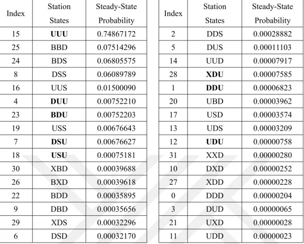
The insights into the why simulation works well for the M/M/1 queue led us to conclude that certain states are never visited. Only those states which are pertinent to the performance measures are visited. The performance of simulation, of course, also depends on the initial state. We next list explicitly the steady-state probabilities of each of the system states to see if there are any states with negligible effects on the performance measure. We select rather realistic parameters. A breakdown probability of 0.01 means that the mean time between failures is 100 cycles. The repair probability is selected to be an order of magnitude larger, corresponding to a mean time to repair of 10 cycles.
Table 2. Steady-State Probabilities of the Production Line Model (q=0.01, r=0.1). Index Station States Steady-State Probability Index Station States Steady-State Probability 15 UUU 0.74867172 2 DDS 0.00028882 25 BBD 0.07514296 5 DUS 0.00011103 24 BDS 0.06805575 14 UUD 0.00007917 8 DSS 0.06089789 28 XDU 0.00007585 16 UUS 0.01500090 1 DDU 0.00006823 4 DUU 0.00752210 20 UBD 0.00003962 23 BDU 0.00752203 17 USD 0.00003574 19 USS 0.00676643 13 UDS 0.00003209 7 DSU 0.00676627 12 UDU 0.00000758 18 USU 0.00075181 31 XXD 0.00000280 30 XBD 0.00039688 10 DXD 0.00000252 26 BXD 0.00039618 27 XDD 0.00000228 22 BDD 0.00035895 0 DDD 0.00000204 9 DBD 0.00035656 3 DUD 0.00000065 29 XDS 0.00032296 21 UXD 0.00000028 6 DSD 0.00032170 11 UDD 0.00000023
The states are arranged so that their steady-state probabilities are in decreasing order. Again, we mark in bold those states where the last machine is productive. It is seen that the steady-state probabilities display a great range of values. The state with the largest probability is UUU with a probability of almost 0.75. The state with the least probability is UDD with a probability of 2.3x10⁻⁷. The difference between the largest and smallest steady-state probability is over six orders of magnitude. That is, the ratio is on the order of a million to one. Clearly, if a simulation runs shorter than a few million cycles, the state UDD with the smallest probability is likely never be visited. This is analogous to not visiting states with more than, say, 100 customers during the simulation of an M/M/1 queue with a traffic intensity of 0.9.
4.2. A TRUNCATED MODEL OF THE THREE STATION PRODUCTION LINE WITH NO BUFFERS
Inspired by our findings in Chapter 3 regarding the M/M/1 queue, now we consider a truncated model of the bufferless three-station line. We truncate the model by
disregarding the states in which more than a single station is under repair. In effect, we are making the seemingly unrealistic assumption that once a station breaks down, the breakdown probability of the other stations is zero. This may seem unreasonable, but it does follow the truncated M/M/1 queue case. There, we make the assumption that once there are some K customers in the system, the arrival rate is zero.
The three-station case can easily be modified to find the production rate of the truncated model. One approach is to start with the steady-state probabilities as computed above. Then, we may remove those states with more than one station under repair, and re-normalize the steady-state vector. Afterwards, we re-compute the production rate.
The systems states with at most one station under repair are listed below. Table 3. States with Fewer than Two Stations Under Repair.
Number of Stations
Under Repair Index
Station States Number of Stations Under Repair Index Station States 0 15 UUU 1 4 DUU 16 UUS 5 DUS 18 USU 7 DSU 19 USS 8 DSS 12 UDU 13 UDS 14 UUD 17 USD 20 UBD 22 BDD 23 BDU 24 BDS 25 BBD
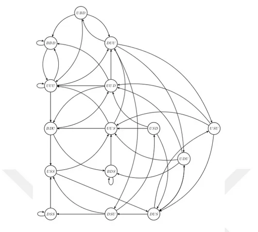
The state transition diagram illustrates the transitions among the systems states of the truncated model.
The states where the last station is operational are marked by bold letters. Note that of the eight such states, we now have only six. The normalization of the steady-state probabilities means we add the steady-state probabilities of the seventeen states shown in Table 3. and then normalize the vector by multiplying it with the reciprocal of the sum of its elements. The production rate is then computed as the sum of the normalized steady-state probabilities of the states shown in bold in Table 3.
The production rate of the truncated model will of course differ from that of the complete model. The question is by how much. We computed the difference for a series of parameters of a three-station bufferless line with identical stations. The differences are given as absolute percentage errors (APE). The absolute percentage error is computed as
APE = 100⋅
|
(production rate )−( production rateof the truncated model)(production rate)
|
. (1)The absolute percentage errors are plotted below.
Figure 8. The State Transition Diagram of the Truncated Bufferless Three Station Model
Figure 9 is rather remarkable. First, observe that the maximum error is about 5.5%. This is actually an extreme case, where both the breakdown and the repair probabilities are 0.1. In this extreme case, the stand-alone availability of a station is 50%. Clearly, in actual implementations, a station would be expected to be operational more than 50% of the time. For realistic cases, that is, where the stand-alone availability is around 90%, the error less than 1%. This is a remarkable phenomenon, that serves not only as an eye-opener, but as motivation to develop practical approximate production line models which are then to be solved algebraically.
4.3. MORE ACCURATE TRUNCATED MODELS OF PRODUCTION LINES WITH NO BUFFERS
Once again, inspired by the results of the preceding section, we now proceed to construct models of production lines where the number of down machines are limited. Analogous to the truncated M/M/1 queue (the M/M/1/K queue), we make the auxiliary assumption that once K of the N stations are down, the remaining stations
become perfectly reliable. Agreeably, this seems like an unjustifiable and quite counterintuitive assumption. The justification lies in the insights hitherto developed – and it is these insights which constitute the contribution of this thesis. In short, we want to remove some of the system states that have probabilities orders of magnitude smaller than others. Obviously, there are many ways to do this pruning. The assumption made here is one approach. It does have the advantage, however, that it is relatively straightforward to model this truncated system, just as it was relatively straightforward to implement the truncated M/M/1 queue.
Software was written to automatically generate the states and the transition probability matrix of bufferless production lines with N stations, but where at most K of the N stations are allowed to be down. We call this the N/K-Truncated-Model. Effectively, once K of the stations are down, the remaining N-K stations are assumed to be perfectly reliable. The states were explicitly obtained by the developed software. A brief overview of the software is given in Appendix 5.
Table 4. Number of System States (N/K models, N stations, at most K down).
N/K 1 2 3 4 5 6 7 8 9 10 3 15 26 32 4 40 92 116 128 5 103 314 435 488 512 6 257 1027 1594 1882 2000 2048 7 623 3218 5665 7133 7833 8096 8192 8 1476 9656 19454 26389 30267 31992 32576 32768 9 3435 27858 64555 131072 10 7882 77694 524288
As seen in Table 4, the number of system states drop considerably when the maximum allowed number of down stations (K) is small. In the extreme case of K=1, we allow only one station to be down at a time. In case of a bufferless production line with 10 stations (N=10), the number of system states goes from 524288 to 7882. This is a 66-fold reduction in the number of system states.
The next investigative question, of course, is “how well does the truncated model approximate the original model?” Here, once again, we develop software to compute
not only the transition probability matrices for the N/K truncated models, but also the production rates. The N/N model gives the production rate of the original models where the number of system states are several orders of magnitude larger. The N/1 truncated models are the approximations. Numerical results are given in the table below.
Table 5. Average Percentage Error of the N/1 Truncated Models. Production Rate (q=0.01, r=0.1)
N N/1 (truncated) N/N (full model) APE 3 0.5166273929 0.5142570532 0.46 4 0.5431647628 0.5388719616 0.80 5 0.5451422158 0.5387804217 1.18 6 0.5375021638 0.5290534472 1.60
As seen from Table 5. the N/1 truncated models provide good approximations to the production rate. The truncated models seem to always over-estimate the production rate. Moreover, the error term seems to increase almost linearly with the number of stations. This can also be used to fine tune the estimates, if our focus were to develop computational methods for the estimation of the production rate. However, our interest in this thesis is more on the conceptual side of the methodologies, as we investigate the ramifications of the models and their use.
5 CHAPTER FIVE
CONCLUSIONS AND FUTURE RESEARCH
In summary, the prominent dominant industrial engineering paradigm in stochastic models of production and service systems calls for the development of various Markovian models whose validation is relegated to simulation studies. Propelled by a paradox that appeared in recent literature (Yeralan & Buyukdagli, 2015) we studied why such simulation gives acceptable results. Our work illustrates that in modeling such industrial engineering systems, there is an agreement between the performance measures and simulation. While other performance measures may not be easily obtained by simulation, measures such as the production rate and the expected number of in-process inventory are congruent to the simulation approach. The simulation community has recognized such shortcomings in general. For example, the topic known as Rare Event Simulation (Bucklew, 2004) dwells on events that have very little probability. However, such body of knowledge does not negate our efforts. It remains that whenever a Markovian model is to be validated by simulation, the applicability and validity of the simulation itself is to be questioned and tested. Again, the validation of simulation may require effort comparable to the validation of the Markov model by other (e.g. analytical) means.
The development of the previous chapters, provides a resolution to our paradox. Indeed, as in the M/M/1 case, simulation does not visit all possible system states. Rather simulation naturally focuses on the system states that have a greater influence on the performance measures. Removing the system states which have negligible effects on the performance measures, we were able to duplicate the results of simulation.
There are significant conclusions to this observation. First, simulation should not be seen as the ultimate verification tool. Its applicability and validity depends on how suitable simulation is to the particular performance measure of interest. For example,
the simulation of an N-station production line will not be able to give an accurate estimate of the probability that all N stations are down, when N is large. In addition, in the numerical examples conducted, it was observed that simulation and exact solutions differ typically by a few percent. Such error ranges are prevalent in the literature. It calls into question that when a study compares its analytical results to simulation and reports errors of a few percent, it may well be that the error is due to simulation rather than the analytical models.
Perhaps the most significant conclusion of this work is in the type of research conducted. The desire to investigate issues other than extensions in the current dominant paradigm. Although it is unlikely to engage in what Kuhn calls extraordinary science at will, without the accompanying serendipity, nonetheless, research is possible to call into question aspects of the dominant paradigm. The major contribution of this work is in that sense. It develops a deeper understanding of a major tool (simulation) in the topic area. Admittedly, it does not trigger the crisis that would challenge the dominant paradigm, it nonetheless provides exploitable avenues in constructing new analytical models (truncated models) which would be expected to perform as well as simulation.
Throughout this study, before focusing on the “simulation paradox” we investigated issues in systems theoretical aspects of manufacturing systems, studied the applicability of predator-prey models in uncovering aspects of cooperation, competition, and co-dependence among companies, and investigated if fractal-like structures in tri-diagonal stochastic matrices could be modeled by use of chaos theory. All of these preliminary works were in fact toward the same goal of attempting to work on something other than what Kuhn calls “normal science”.
REFERENCES
Altiok, T. (1996). Performance Analysis of Manufacturing Systems. Springer.
Anonymous Academic. (2014). What Do Uni Engineering Departments Need Most? People in Overalls. Retrieved 3 May 2016, from
http://www.theguardian.com/higher-education-network/2014/nov/21/university-engineering-departments-overalls-research
Askin, R. G., & Standridge, C. R. (1993). Modeling and Analysis of Manufacturing Systems (1st ed.). Wiley.
BLAS. (2015). Retrieved 3 April 2016, from http://www.netlib.org/blas/
Boehm, V. R. (1980). Research in the ‘Real World’ - A Conceptual Model. Personnel Psychology, 33(3), 495–503. http://doi.org/10.1111/j.1744-6570.1980.tb00479.x Bucklew, J. A. (2004). Introduction to Rare Event Simulation. New York, NY:
Springer New York. http://doi.org/10.1007/978-1-4757-4078-3
Burden, R. L., & Faires, J. D. (2010). Matrix Factorization. In Numerical Analysis (9th ed., p. 900). Brooks/Cole, Cengage Learning. Retrieved from
http://ins.sjtu.edu.cn/people/mtang/textbook.pdf
Buzacott, J. A., & Shanthikumar, J. G. (1993). Stochastic Models of Manufacturing Systems. Prentice Hall.
Byrd, D. (2010). Zeno s " Achilles and the Tortoise " Paradox and The ʼ Infinite Geometric Series. Retrieved from
http://homes.soic.indiana.edu/donbyrd/Teach/Math/Zeno+Footraces+InfiniteSeri es.pdf
Cantini, A. (2007). Paradoxes and Contemporary Logic. Retrieved 21 October 2015, from http://plato.stanford.edu/entries/paradoxes-contemporary-logic/#Int
Costa, A. L. (1985). Developing Minds: A Resource Book for Teaching. (A. L. Costa, Ed.)Educational Leadership (Vol. 1). ASCD.
Critical Thinking Community. (n.d.). Defining Critical Thinking. Retrieved 13 October 2015, from https://www.criticalthinking.org/pages/defining-critical-thinking/766
Cucic, D. A. (2009). Types of Paradox in Physics. 0912.1864. Retrieved from http://arxiv.org/abs/0912.1864\nhttp://www.arxiv.org/pdf/0912.1864.pdf Dowden, B. (n.d.). Zeno’s Paradoxes. In Internet Encyclopedia of Philosophy.
Economist. (2010). The Disposable Academic. Retrieved 3 May 2016, from http://www.economist.com/node/17723223
Eliason, J. L. (1996). Using Paradoxes to Teach Critical Thinking in Science. Journal of College Science Teaching, 15(5), 341–44. Retrieved from http://eric.ed.gov/? id=EJ520704
Engineering, R. A. of. (2010). Philosophy of Engineering. Philosophy of
Engineering: Proceedings of a Series of Seminars Held at The Royal Academy of Engineering, 1, 76. http://doi.org/10.1016/B978-0-12-385878-8.00001-X Felkins, L. (1995). Paradoxes and Dilemmas. Retrieved 21 October 2015, from
http://perspicuity.net/paradox/paradox.html
GCC. (2016). Retrieved 20 March 2016, from https://gcc.gnu.org/
Gershwin, S. B. (1994). Manufacturing Systems Engineering. Prentice Hall. Gershwin, S. B., & Schick, I. C. (1983). Modeling and Analysis of Three-Stage
Transfer Lines with Unreliable Machines and Finite Buffers. Operations Research, 31(2), 354–380. http://doi.org/10.1287/opre.31.2.354
GSL. (2009). Retrieved 15 March 2016, from http://www.gnu.org/software/gsl/ Hansen, H. (2015). Fallacies. In Stanford Encyclopedia of Philosophy. Retrieved
from http://plato.stanford.edu/entries/fallacies/#ForAppInfFal
Hillier, F. S., & Lieberman, G. J. (2009). Introduction to Operations Research (9th ed.). McGraw-Hill Science/Engineering/Math.
John Fowles. (1985). The Magus (Revised). Dell.
Jon Excell. (2013). Academia’s Engineering Skills Shortage. Retrieved 3 May 2016, from https://www.theengineer.co.uk/issues/december-2013-online/academias-engineering-skills-shortage/
Kuhn, T. S. (1970). The Structure of Scientific Revolutions. Philosophical Review (Vol. II). http://doi.org/10.1119/1.1969660
Li, J., & Meerkov, S. M. (2009). Production Systems Engineering. Springer. Maggio, N., Matta, A., Gershwin, S. B., & Tolio, T. (2009). A decomposition
approximation for three-machine closed-loop production systems with unreliable machines, finite buffers and a fixed population. IIE Transactions, 41(6), 562–574. http://doi.org/10.1080/07408170802714695
Muth, E. J. (1979). The Reversibility Property of Production Lines. Management Science, 25(2), 152–158. http://doi.org/10.1287/mnsc.25.2.152
that are subject to breakdown. In 1981 20th IEEE Conference on Decision and Control including the Symposium on Adaptive Processes (pp. 643–648). IEEE. http://doi.org/10.1109/CDC.1981.269288
Panda, A., & Gupta, R. K. (2014). Making academic research more relevant: A few suggestions. IIMB Management Review, 26(3), 156–169.
http://doi.org/10.1016/j.iimb.2014.07.008
Papadopolous, H. T., Heavey, C., & Browne, J. (1993). Queueing Theory in Manufacturing Systems Analysis and Design (1st ed.). Chapman & Hall/CRC. Paul, R. W. (1991). Teaching Critical Thinking In Strong Sense. In A. L. Costa (Ed.),
Developing Minds: A Resource Book for Teaching Thinking (Revised Ed, pp. 77 – 85). Alexandria, VA: ASCD.
Quine, W. (1966). The Ways of Paradox. The Ways of Paradox and Other Essays, 3– 20.
Schick, I., & Gershwin, S. (1978). Modelling and analysis of unreliable transfer lines with finite interstage buffers. Complex Material Handling and Assembly
Systems, 6.
Silagadze, Z. K. (2005). Zeno meets modern science. Acta Physica Polonica B, 36(10), 2887–2929.
Tempelmeier, H., & Kuhn, H. (1993). Flexible Manufacturing Systems (1st ed.). Wiley-Interscience.
Yeralan, S., & Buyukdagli, O. (2015). The Ontology of Large-Scale Markovian models. In Stochastic Models of Manufacturing and Service Operations. Yeralan, S., Franck, W. E., & Quasem, M. A. (1986). A continuous materials flow
production line model with station breakdown. European Journal of Operational Research, 27(3), 289–300. http://doi.org/10.1016/0377-2217(86)90326-7
Yeralan, S., & Tan, B. (1997). Analysis of multistation production systems with limited buffer capacity part 1: The subsystem model. Mathematical and Computer Modelling, 25(7), 109–122. http://doi.org/10.1016/S0895-7177(97)00052-6
APPENDIX 1 – CRITICAL THINKING
Critical thinking helps us to determine whether a given argument is valid or not. An argument is a set of premises (statements) that together comprise reason for a conclusion (another statement). This decision mechanism is based upon the logical and structural validity of the given statements, that is, whether the statements necessarily lead to the conclusion. When all of the premises are true, the conclusion must be true for the argument to be valid. For instance, your best friend told you that he cannot make it to the Broadway show tonight. When you asked him the reason, he might give these arguments: (a) that it is the end of the month and he ran out of money, (b) that he broke his arm, and it is casted or (c) that he just found out that the leading actress on the show is his ex-girlfriend.
The first argument seems possible to you, because you know it is the end of the month, and your friend does not know how to manage his money. It is a reasonably good argument which has nothing to do with morality, but directs us to a probable conclusion.
If your friend broke his arm, it is probably a good argument, which leads to a rational but not to an absolute conclusion. Even if it is true, your friend may take some pain killers and make it to the show if it is really important to you. Therefore it is an ampliative argument.
And the lie that the beautiful, talented, leading actress on the show is your best friend's ex-girlfriend? It is a very, very bad argument obviously, because he is not that handsome, or wealthy, or clever. He is probably lying to you because he does not want you to know the real reason of why he cannot come. So why do you not be a good friend and treat him to the play by buying the tickets, or if he really broke his arm, pay him a visit with a bottle of red wine to make a movie night at home.
But sometimes, we can detect an incorrect conclusion from the arguments. Mistakes that we make unintentional or intentional (unfortunate but abundant examples can be seen in politics, or commercials, etc.) in critical thought is called fallacies. Dowden (n.d.) explains that there is an abundance of definitions for the term “fallacy”, since