Selçuk J. Appl. Math. Selçuk Journal of Special Issue. pp. 21-33, 2011 Applied Mathematics
The Mixed Weibull-Negative Binomial Distribution Mustafa Ça˘gatay Korkmaz1, Co¸skun Ku¸s2, Hamza Erol3
1Artvin Çoruh University Faculty of Art&Science Department of Statistics 08000
Artvin, Turkiye
e-mail:m cagatay@ artvin.edu.tr
2Selçuk University Faculty of Science Department of Statistics 42075 Konya, Turkiye
e-mail:.coskun@ selcuk.edu.tr, agenc@ selcuk.edu.tr
3Çukurova University Faculty of Art&Science Department of Statistics 01100 Adana,
Turkiye
e-mail:.herol@ cu.edu.tr
Abstract. In this paper, we introduce the Weibull Negative Binomial (WNB) with four parameters distribution which is obtained by compounding Weibull and Negative Binomial distributions, where compounding procedure follows same way that was previously carried out by Adamidis and Loukas (1998) and Kus (2007). This new distribution is a genaral case Exponential-geometric (EG) and Weibull-geometric distributions (WG), which was introduced recently by Adamidis and Loukas (1998) and Barreto-Souza et. all. (2010) respectively. The WNB distribution has increasing, decreasing, upside down bathtub hazard function. We obtain several properties of the WNB distributions such as mo-ments, order statistics, estimation by maximum likelihood and inference for large sample. Furthermore, EM algorithm is also used to determine the maximum likelihood estimates of parameters and we discuss Renyi and Shannon entropy. Applications to real data sets are given to show the exibility and potentiality of the proposed distribution.
Key words: Compounding; Mixed distribution; Failure rate; EM algorithm; Weibull distribution; Lifetime distributions; Maximum likelihood estimation; Negative Binomial distribution.
2000 Mathematics Subject Classification: 462F30. 1. Introduction
Two-parameter distributions to model lifetime data have been introduced by compounding exponential and power series distributions. The exponential geo-metric (EG), exponential Poisson (EP) and exponential logarithmic (EL) dis-tributions were introduced and studied by Adamidis and Loukas (1997), Kus (2007) and Tahmasbi and Rezaei (2008) respectively. Recently, Chahkandi and
Ganjali (2009) introduced the exponential power series (EPS) distributions, which contains these distributions. Proschan (1963) proved that decreasing hazard function is inherent to mixtures of distributions with constant hazard function (see also McNolty et al., 1980 for other properties of exponential mix-tures) and Gleser (1989) demonstrated the converse for any gamma distribution with shape parameter less than one. Extensions of the EP and EG distributions were proposed by Barreto-Souza and Cribari-Neto (2009) and Silva et al. (2009) with the generalized exponential Poisson and generalized exponential geometric distributions, respectively. Their hazard functions may take the form increasing, decreasing and upside down bathtub. Chahkandi and Ganjali (2009), studied by compounding exponential and power series EPS distributions which contains several distributions which have been introduced and studied such as: EG, EP, EB (Exponential-Binomial) and EL distributions. The EPS distributions have decreasing hazard function. Korkmaz (2010) studied the Exponential-Negative Binomial Distribution and studied several of its properties in his master thesis. Also, Weibull-Geometric (WG) distribution and Weibull-Power Series (WPS) distributions were studied Souza et al. (2010), Morais and Barreto-Souza (2011) respectively. WPS distributions generalize the EPS distributions. WPS distributions has decreasing, upside down bathtube hazard function. In this paper we introduce Weibull-Negative Binomial (WNB) with four parame-ters distribution which is obtained by compounding Weibull and Negative Bino-mial distributions. The WNB of distributions contains EG, WG, Exponential-Negative Binomial (ENB) distributions. Unlike EPS distributions, further de-creasing hazard functions, our distribution has associated hazard function as-suming the forms increasing, upside down bathtub etc. The paper is organized as follows. In the Section 2, we define the WNB distribution. In Section 3, prop-erties such as quantiles, moments and order statistics are obtained., we present Renyi and Shannon entropies of the WNB distribution in section 4. Further, estimation of the parameters by maximum likelihood and via the EM algorithm are presented in the Section 5. Inference for large sample is discussed in Section 6. A application to a real data set in Section 7. Concluding remarks are given in the Section 8.
2. The Distribution
Let Y1, Y2, ..., YZ be independent and identically distributed (iid) random vari-ables following the Weibull distribution whose density is given by
g (y; α, β) = βαβyβ−1e−(yα)β, y > 0, α, β > 0.
Here, Z is a discrete random variable following Negative-Binomial distribution with probability function given by
P (Z = z) = µ z − 1 k − 1 ¶ (1 − p)kpz−k, z = k, k + 1, ... , k ∈ N+, p ∈ (0, 1) .
Z and Ys are independent to be let X = min {Yi}Zi=1.The conditional cumula-tive distribution function (cdf) of X|Z = z is given by
FX|Z=z(x) = 1 − e−z(xα)
β
.
X|Z = z follows a Weibull distribution with parameters αz1/βand β. The marginal distribution function of X given by
(1) F (x) = 1 − (1 − p)ke−k(xα)
β
(1 − pe−(xα)β)−k, x > 0, α, β > 0, p ∈ (0, 1), k ∈ N+
We denote a random variable X following WNB distribution with parameters α, β, p and k by X ∼ W NB(θ), where θ = (α, β, p, k) parameters vector. This distribution generalizes several distributions which has been introduced and studied in the literature. The EG distribution (Adamidis and Loukas, 1998) and WG distribution (Barreto-Souza et all. 2010) are special case of WNB distribution when k = 1, β = 1 and k = 1 respectively. Exponential-Negative Binomial (ENB) distribution ,which studied by Korkmaz’s master thesis (2010), obtains while β = 1. Moreover, while p → 0 The WNB distribution convergences weibull distribution with parameters αk1/βand β parameters.
3. Proporties of WNB Distribution
The probability density function (pdf) associated to (1) is given by (2) f (x; θ) = βαβkxβ−1(1 − p)ke−k(xα)β³1 − pe−(xα)β´−(k+1), x > 0, and survival function is
S(x) = (1 − p)ke−k(xα)β(1 − pe−(xα)β)−k, x > 0.
Proposition 1. The pdf of a WNB distribution is monotone decreasing if β ≤ 1 and unimodal if β > 1.
Proof. We have that
∂ log f (x)
∂x = 0 ⇒ x
∗= α−1(β − 1 βk )
−β If β ≤ 1, x∗do not have solution for α > 0 and k ∈ N
+. Therefore pdf can only monotone decreasing. If β > 1, x∗ exists, unique and modal value. Moreover, ∂2log f (x)/∂x2|
x=α−1(β−1
βk )−β < 0 and hence f is unimodal. This proof was done
can be shown an an infinite mixture of Weibull distributions with same shape parameter β. If |a| < 1 and n > 0, we have the series representation
(3) (1 − a)−n= ∞ X j=0 µ n + j − 1 j ¶ aj. We expand³1 − pe−(xα)β´−(k+1)
as in Equation (3) and then the density func-tion of WNB distribufunc-tion can be written
f (x; θ) = βαβkxβ−1(1 − p)ke−k(xα)β ∞ X j=0 µ k + j j ¶ pje−j(xα)β. Using Weibull density we obtain,
(4) f (x; θ) = k(1 − p)k ∞ X j=0
pjg(x; α(k + j)1/β, β).
So, properties of the WNB distribution can be obtained from Weibull distribu-tion.
The hazard function is given by
h (x; θ) = kβαβxβ−1³1 − pe−(xα)β´−1
, x > 0.
We have that limx→0h(x) = 0 and limx→∞h(x) = ∞, thus the failure rate function is ultimately increasing, so a pure bathtub form is imposibble (this is conceptually appealing in contrast with, say, the decreasing Weibull distribution where h(0) = ∞, h(∞) = 0).
Proposition 2If β ≤ 1 , the hazard function is decreasing. Proof. We have that
η(x) = −f´(x)/f(x) = βαβxβ−1³k + pe−(xα)β´ ³1 − pe−(xα)β´−1, x > 0. Hence, the first derivative of η(.) is given by
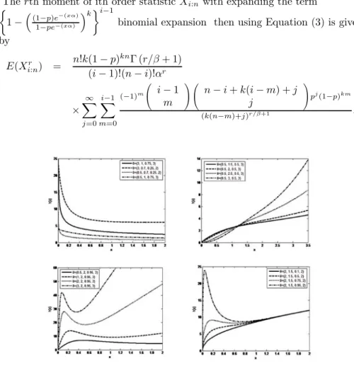
η´(x) = βu£(1 − β)¡p2e−2u+ p(k − 1)e−u− k¢− upβ(k + 1)e−u¤× × [x (1 − pe−u)] , x > 0, where u = (xα)β. If β ≤ 1, we obtain η´(x) < 0, ∀x > 0. Therefore, the result follows from Glaser’s Theorem (1980). However, for other parameter values, it can take different forms. Figure 2 illustrates some of the possible shapes of the hazard function for selected values of the parameters vector. These plots show that the hazard function of the new distribution is much more flexible than the EG and WG distributions.
3.1. Quantiles and Moments
The ξth quantil of WNB distribution is given by
xξ = α−1 ⎧ ⎨ ⎩log ⎛ ⎝1 − p ³ 1 − (1 − ξ)1/k´ (1 − ξ)1/k ⎞ ⎠ ⎫ ⎬ ⎭ 1/β .
In particular, the median is simply x0.5= α−1
n
log³21/k(1 − p) + p´o1/β.
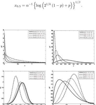
Figure 1. Plots of density WNB distribution selected special values.
The r th moment of X is given by using Equaiton (4) and transforming u = (xα)β E(Xr) = k(1 − p)kα−rΓ¡1 + rβ−1¢ ∞ X j=0 µ k + j j ¶ pj(k + j)−(1+rβ−1),
3.2. Order Statistics
Order statistics make their appearance in many areas of statistical theory and practice. First, we derive the density of order statistics. Let X1, X2, ..., Xn be iid random variables WNB distribution. The density of the i th order statistics is given by fi:n(x) = n!kβαβxβ−1(1 − p)k(n−i+1)(xα)βe−k(n−i+1)(xα)β (i − 1)!(n − i)!(1 − pe−(xα)β )n−i+k+1 × × ( 1 − µ (1 − p)e−(xα) 1 − pe−(xα) ¶k)i−1 , x > 0. The rth moment of ith order statistic Xi:nwith expanding the term ½
1 −³(11−p)e−pe−(xα)−(xα)
´k¾i−1
binomial expansion then using Equation (3) is given by E(Xi:nr ) = n!k(1 − p) knΓ (r/β + 1) (i − 1)!(n − i)!αr × ∞ X j=0 i−1 X m=0 (−1)m ⎛ ⎝ i − 1 m ⎞ ⎠ ⎛ ⎝ n − i + k(i − m) + j j ⎞ ⎠pj(1 −p)km (k(n−m)+j)r/β+1 .
Figure 2.Plots of hazard rate function WNB distribution selected special values.
An alternative expression to Equation (5) can be obtained by using result due to Barakat and Abdelkader (2004). This expression is
E(Xi:nr ) = r n X m=n−i+1 (−1)m−n+i−1 µ m − 1 n − i ¶ µ n m ¶Z∞ 0 xr−1S (x)mdx,
where, S(x) is the survival function. Using expansion (3) and changing variables u = (xα)β, we obtain ∞ Z 0 xr−1S (x)mdx = (1 − p) kmΓ (r/β) αrβ ∞ X j=0 µ km + j − 1 j ¶ pj (km + j)r/β. Hence, E(Xi:nr ) = Γ (r/β + 1) (−1)n−i+1 × ∞ X j=0 n X m=n−i+1 (−1)m µ m − 1 n − i ¶ µ n m ¶ µ km + j − 1 j ¶ (1−p)kmpj (km+j)r/β.
4. Rényi and Shannon Entropies
Entropy has been used in various situations in science and engineering. The entropy of a random variable X is a measure of variation of the uncertainty. The Rényi entropy is defined by IR(γ) = 1/(1 − γ) log©RRfγ(x)dxª, for γ > 0 and γ 6= 1. We can use Equation (3) and obtain
∞ Z 0 fγ(x) dx =nβk (1 − p)k αβoγ ∞X j=0 µ γ (k + 1) + j − 1 j ¶ pj× × ∞ Z 0 xr(β−1)e−(kγ+j)(xα)β dx
If (β − 1) (γ − 1) º 0, and using u = (xα)βtransforming this expression reduces to ∞ Z 0 fγ(x) dx = nk (1 − p)ko γ (αβ)γ−1Γ µ (β − 1) (γ − 1) β + 1 ¶ × ∞ X j=0 µ γ (k + 1) + j − 1 j ¶ (kγ + j)(β−1)(γ−1)β +1 pj.
Thus we have IR(γ) = 1/(1 − γ) log ⎧ ⎪ ⎪ ⎪ ⎪ ⎨ ⎪ ⎪ ⎪ ⎪ ⎩ n k (1 − p)ko γ (αβ)γ−1Γ³(β−1)(γ−1)β + 1´ × ∞ X j=0 ⎛ ⎝ γ (k + 1) + j − 1 j ⎞ ⎠ (kγ+j)(β−1)(γ−1)β +1 pj ⎫ ⎪ ⎪ ⎪ ⎪ ⎬ ⎪ ⎪ ⎪ ⎪ ⎭ .The Shannon entropy is defined by E {− log f (X)}. This is special case derived from limγ→1IR(γ). Hence,
E {− log f (X)} = − log³βk (1 − p)kαβ´− (β − 1) E (log X) + kαβE¡Xβ¢ + (k + 1) E³logn1 − pe−(Xα)βo´. Further, E (log X) = −k (1 − p) k β ∞ X j=0 µ k + j j ¶ pjlog©αβ(k + j)ª+ ζ (k + j) , E¡Xβ¢= (1 − p) k kαβ F2,1([k, k] , [k + 1] , p) , E³logn1 − pe−(Xα)βo´= k (1 − p)k ∞P j=0 µ k + j j ¶ pjR∞ 0
log¡1 − pe−u¢e−u(k+j)du, where, ζ is Euler’s constant and Fp,q([n] , [d] , λ) is the generalized hyperge-ometric function. This function is also known as Barnes’s extended hypergeo-metric function. The definition of Fp,q([n] , [d] , λ) is
Fp,q([n] , [d] , λ) = ∞ X j=0 λj p Y i=1 Γ (ni+ j) Γ−1(ni) Γ (j + 1) q Y i=1 Γ (di+ k) Γ−1(di) ,
where n = [n1, n2, ..., np], p is the number of operands of n, d = [d1, d2, ..., dq] and q is the number of operands of d. Generalized hypergeometric function is quickly evaluated and readily available in standard software such as Maple. 5. Estimation
Let X1, X2, ..., Xn be a random sample of the WNB distribution with parameter vector θ = (α, β, p, k). The log-likelihood function = (θ, x) ,
= n log β + n log k + kn log(1 − p) + nβ log α + (β − 1) n X i=1 log xi −kαβ n X i=1 xβi − (k + 1) n X i=1 log³1 − pe−(xα)β´
and the associated gradients are found to be ∂l ∂p = −kn(1 − p) −1+ (k + 1) n X i=1 e−(xiα)β(1 − pe−(xiα)β)−1 ∂l ∂α = nβα −1− βαβ−1 n X i=1 xβi(k + pe−(xiα)β)(1 − pe−(xiα)β)−1 ∂l ∂β = nβ−1+n log α+ n X i=1 log xi−αβ n X i=1 xilog(xiα)(k+pe−(xiα) β )(1−pe−(xiα)β)−1.
Gradient equation for k isn’t written because of k is integer value. Therefore, within a set of values of k, which maximizes the likelihood function will be appropriate k value. k ’s selection process focused on the practice side. The maximum likelihood estimates of θ is calculated numerically so we propose the use of the EM algorithm (Dempster et al., 1977). For doing this, we define complete data distribution with density function
f (x, z; θ) = zβαβ µ z − 1 k − 1 ¶ (1 − p)kpz−kxβ−1e−z(xα)β
for x > 0, α, β > 0, p ∈ (0, 1) , z = k, k + 1, ..., k ∈ N+. The E-step of EM algorithm requries the conditional expectation of ³Z|X; θ(r)´, where θ(r) = ³
α(r), β(r), p(r)´ is current estimate of θ. From,
P (z|x; θ) = µ z k ¶ ³ pe−(xα)β´z−k³1 − pe−(xα)β´k+1
for z = k, k+1, ..., k ∈ N+. We have E(Z|X; θ) = (k+pe−(xα)
β
)(1−pe−(xα)β)−1. The E-step is completed. Now we apply M-step by using the maximum like-lihood estimation over θ. The missing Z’s is replaced to maximum likelike-lihood estimation of θ based on complete data distribution. Hence the EM iteration is obtained that p(r+1) = 1 − nk à n X i=1 z(r)i !−1 , α(r+1)= n1/β(r+1) à n X i=1 zi(r)xβi(r+1) !−1/β(r+1) ,
where β(r+1) is the solution of the nonlinear equation nβ(r+1)−1+ n log α(r+1)+ n X i=1 log(xi) − α(r+1) β(r+1)Xn i=1 z(r)i xβi(r+1)log(xiα) = 0 where, zi(r)= (k + p(r)e−(xiα(r))β(r))(1 − p(r)e−(xiα(r))β(r))−1, i = 1, 2, .., n.
6. Inference
For interval estimation and hypothesis tests on the model parameters, we obtain the 3 × 3 observed information matrix Jn= Jn(θ) given by
Jn = ⎛ ⎝ IIpppβ IIpββ IIpβα Ipα Iβα Iαα ⎞ ⎠ , where, Ipp= − ∂2 ∂p2 = n(1 − p)−2− (k + 1) n X i=1 e−2(xiα)β (1 − pe−(xiα)β)−2 Ipα= − ∂2 ∂p∂α= βα β−1(k + 1) n X i=1 xβie−(xiα)β (1 − pe−(xiα)β)−2 Ipβ= − ∂2 ∂p∂β = (k + 1) n X i=1 (αxi)βlog (αxi) e−(xiα) β (1 − pe−(xiα)β)−2 Iαα = − ∂2 ∂α2 = nβ α2 + βα β−2(β − 1) × ⎧ ⎪ ⎪ ⎪ ⎨ ⎪ ⎪ ⎪ ⎩ n X i=1 xβi(k + pe−(xiα)β)(1 − pe−(xiα)β)−1 −pβ(k + 1)αβ n X i=1 x2βi e−(xiα)β(1 − pe−(xiα)β)−2 ⎫ ⎪ ⎪ ⎪ ⎬ ⎪ ⎪ ⎪ ⎭ Iαβ= − ∂ 2 ∂α∂β = −n α+α β−1 ½ (β log α + 1) n P i=1 xβi(k + pe−(xiα)β )(1 − pe−(xiα)β)−1 ¾ −βαβ−1 ( n P i=1 xβi p2e−2(xiα) β
log xi+pe−(xiα) β
[(k+1)(αxi)βlog (αxi)+(k−1) log xi]−k log xi
(1−pe−(xiα)β)2 ) Iββ= −∂ 2 ∂β2 = n β2+αβ ½ log α n P i=1 xβi log (αxi)(k + pe−(xiα)β )(1 − pe−(xiα)β)−1 ¾ −αβ ( n P i=1 xβilog (αxi) p 2
e−2(xiα)βlog xi+p{(k+1)(αxi)βlog(αxi)+(k−1) log xi}−k log xi
(1−pe−(xiα)β)2
) .
Under conditions that are fulfilled for the parameter θ in the interior of the para-meter space but not on the boundary, the asymptotic distribution of√n³bθ − θ´is
multivariate normal N3 ³
0, K−1³bθ´´, where K(θ) = limn
→∞n−1Jn(θ) is the unit information matrix. This asymptotic behaviour remains valid if K(θ) is re-placed by the average sample information matrix evaluated at θ, say n−1J
n(bθ). We can use the approximate multivariate normal N3
³ 0, Jn−1
³
bθ´´ distribution of bθ to construct approximate confidence regions for some parameters and for the hazard and survival functions. In fact, an 100(1−γ)% asymptotic confidence interval for each parameter θiis given by
ACIi= ³ bθ − zγ/2 p b Jθiθi , bθ + z γ/2 p b Jθiθi ´ , where bJθiθi represents the (i, i) diagonal element of J−1
n ³
bθ´ for i = 1, 2, 3, and zγ/2is the quantile 1 − γ/2 of the standard normal distribution.
The likelihood ratio (LR) statistic is useful for comparing the WNB distribution with some of its special sub-models. We consider the partition θ = (θT1, θT2)T of the WNB distribution, where θ1 is a subset of parameters of interest and θ2 is a subset of the remaining parameters. The LR statistic for testing the null hypothesis H0 : θ1 = θ(0)1 versus the alternative hypothesis H0 : θ1 6= θ(0)1 is given by w = 2nl³bθ´− l¡θ¢o, where θ and bθ are the MLEs under the null and alternative hypotheses, respectively. The statistic w is asymptotically (as n → ∞) distributed as χ2k, where k is the dimension of the subset θ1of interest. 7. Application
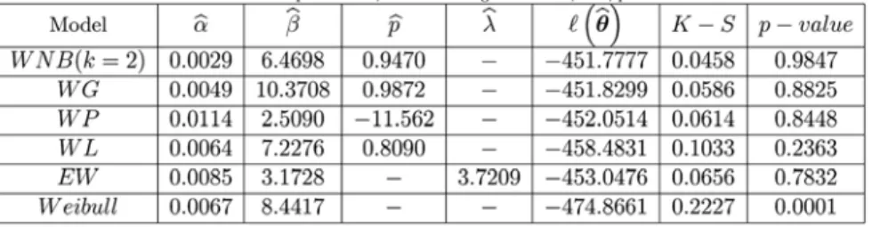
In this section, we fit the WNB, WG, WP Poisson), WL (Weibull-Logarithmic), Weibull models to a real data set. WP and WL models has been studied by Morais and Barreto-Souza (2011). We also fit the three-parameter ex-ponentiated Weibull (EW) distribution introduced by Mudholkar and Srivastava (1993) to make a comparison with the WNB models. The cdf of the EW distri-bution is given by F (x; β, α, λ) =¡1 − e−(βx)α¢λ, x > 0,with β, α, λ > 0.The data set is given by Birnbaum and Saunders (1969) on the fatigue life of 6061-T6 aluminum coupons cut paralel to the direction of rolling and oscillated at 18 cycles per second. The data set consists of 101 observations with maximum stres per cycle 31,000 psi. The data are: 70, 90, 96, 97, 99, 100, 103, 104, 104, 105, 107, 108, 108, 108, 109, 109, 112, 112, 113, 114, 114, 114, 116, 119, 120, 120, 120, 121, 121, 123, 124, 124, 124, 124, 124, 128, 128, 129, 129, 130, 130, 130, 131, 131, 131, 131, 131, 132, 132, 132, 133, 134, 134, 134, 134, 136, 136, 137, 138, 138, 138, 139, 139, 141, 141, 142, 142, 142, 142, 142, 142, 144, 144, 145, 146, 148, 148, 149, 151, 151, 152, 155, 156, 157, 157, 157, 157, 158, 159, 162, 163, 163, 164, 166, 166, 168, 170, 174, 201, 212. This data set have been analyzed recently by Barreto-Souza et al.(2009) and Morais and Barreto-Souza (2011). From 1 through 15 for the values of k, the log-likelihood function is calculated and the maximum log-likelihood value given k which is chosen as appropriate for WNB model. Therefore, the log-likelihood value is maximum
for k =2. Plot of log-likelihood values for selected k values is given in Figure 3. Table 1 shows the MLEs of the parameters, the maximized log-likelihood, K-S and p values for the WNB, WG, WP, WL, EW and Weibull models. In table 1, these values are the best for WNB model among other models. Plot of the density of the fitted WNB model is given in Figure 4. The LR statistics for testing the null hypotheses Ho: W eibull against the alternative hypothesis H1: W N B is 46.1822 (p-value=1.07×10⁻¹¹) . Hence, for any usual significance level, we reject null distribution in favour of the WNB distribution.
8. Conclusions
We define a new model, so-called the WNB distribution, that generalizes , the EG distribution introduced by Adamidis and Loukas (1998) and the WG tribution introduced by Morais and Barreto-Souza (2010) and the Weibull dis-tribution. Plots of the density and hazard functions are presented. The WNB distribution, while more complicated, appears more flexible in the behaviour of its hazard function.Various standard mathematical properties are derived.We obtain closed form expressions for the moments, the density of order statistics and expansions for their moments. Maximum likelihood estimation is discussed and an EM algorithm is proposed. We discuss asymptotic likelihood inference including confidence intervals for the model parameters and the LR statistics to compare the WNB model with its special sub-model. Finally, we fitted the WNB model to a real data set to show the potentially of the new distribution.
Figure 3. log-likelihood values for selected k values
Figure 4. The fitted WNB densities for the data set
Table 1. MLE’s of the models parameters, maximized log-likelihoods, K-S, pvalues
References
1. Adamidis, K., Loukas, S., (1998) . “A lifetime distribution with decreasing failure rate. Statistics and Probability Letters”, 39, 35-42.
2. Barakat, H.,M., Abdelkader, Y., H., (2004). “Computing the moments of order statistics from nonidentical random variable”, Statistical Methods and Applications 13, 15-26.
3. Barreto-Souza, W., Cribari-Neto, F., 2009. “A generalization of the exponential— Poisson distribution”. Statistics & Probability Letters 79, 2493—2500.
4. Barreto, W., S., Morais, L., A., Cordeiro, M., G., (2010). “The Weibull-geometric distribution”. Journal of Statistical Computation and Simulation, 81, 645-657. 5. Birnbaum, Z.W., Saunders, S.C., 1969. “Estimation for a family of life distributions with applications to fatigue”. Journal of Applied Probability 6, 328—347.
6. Chahkandi, M., Ganjali, M., (2009). “On Some lifetime Distributions with decreas-ing failure rate”, Computational Statistics and Data Analysis, 53, 4433-4440. 7. Dempster, A., P., Laird, N., M., Rubin, D., B., (1977). “Maximum likelihood from incomplete data via the EM algorithm”, J. Roy. Stat. Soc. Ser. B, 39, 1-38.
8. Glaser, R.E., 1980. “Bathtub and related failure rate characterizations”. Journal of the American Statistical Association 75, 667—672.
9. Korkmaz, M., Ç., (2010). “ A new Three Parameters life time distribution wıth decrasing failure rate” Selçuk University Science Institute unpublished Master thesis, Konya.
10. Ku¸s, C., (2007). “A new lifetime distribution”. Computational Statistics and Data Analysis, 51, 4497-4509.
11. McLachlan, G., J., Krishnan, T., (1997). “The EM Algorithm And Extension”, Wiley, New York.
12. Morais, L., A., Barreto, W., S., (2011). “A Compound class of weibull and power series distributions”, Computational Statistics and Data Analysis, 55, 1410-1425. 13. Mudholkar, G.S., Srivastava, D.K., 1993. “Exponentiated Weibull family for analyzing bathtub failure-rate data”. IEEE Transactions on Reliability 42 (2), 299— 302.
14. Shannon, C.E., 1948. “A mathematical theory of communication”. Bell System Technical Journal 27, 379—432.
15. Silva, R.B., Barreto-Souza, W., Cordeiro, G.M., 2010. “A new distribution with decreasing, increasing and upside-down bathtub failure rate”. Computational Statis-tics & Data Analysis 54, 935—944.
16. Tahmasbi, R., Rezaei, S., (2008). “A two parameters lifetime distribution with decreasing failure rate”, Computational Statistics and Data Analysis, 52, 3889-3901.