íiu· .- л»·^^ ·.· ·' - 1! ‘ η V'/ .V ‘ Ч 'г ^' : ,f · М ·«· . ■«■'‘í.«.‘ '.ví* ií,' 'Ä -a* r„v ч Ч.· ü, *■·- _ ■ Яі!· ' .. e ■ # 1 -:í« í, ’ . / V ήι*·^··;.·Γ<^:ΐ ·:?··» îRİf'.|§'->r*iWİ ?ft**4··· я . W<îi· i’ · ··«’ ■» '-’W· ‘W ** r •■■•A.^· -v>-¿· « . ι^.·:^^γΙ «P* I Г ^-·· £і%Л W |. .S. 1.1 i. 2 W*. ir. ■«^ ',·\ .,.>·:·:?···.· ·-ЛіХ ■· ·ν · · .·/ ·#»4 а ϊ ^Í
ABC INVENTORY C LA SS IF I C A T I O N AN APPLICATION:
O ZDEMIRLER
A THESIS
SUBMITTED TO THE DEPARTMENT OF MANAGE M E N T
AND THE INSTITUTE OF
MANAGEMENT SCIENCES
OF BILKENT U N I V E R S I T Y
IN PARTIAL F U L LFILLMENT OF THE REQU I R E M E N T S FOR THE DEGREE OF
MASTER OF BUSINESS A DM IN I S T R A T I O N oy MEHMET DURU January, 1989 ____________
tarafmdän ba^i5İaniüiştır,
ИР
5
' S S D 3 3 9 1 aç's^ *C73
I certify that I have read this thesis and that in my opinion
it
is fully adequate,
in scope and in quality,
as a thesis
for the degree of Master of Business Administration.
-v:.
Assist. Prof. Erdal Erel
I certify that I have read this thesis and that in my opinion
it
is fully adequate,
in scope and in quality,
as a thesis
for the degree of Master of Business Administration.
Assist. Prof. Dilek Yeld an
I certify that I have read this thesis and that in my opinion
it
is fully adequate,
in scope and in quality,
as a thesis
for the degree of Master of Business Administration.
3^.
Assist. Prof. Kursat Aydogan
Approved for the Institute of Management Sciences
c
Prof. Dr. Siibidey Togan
ABSTRACT
ABC INVENTORY CLASSIFICATION AN APPLICATION:
OZDEMIRLER
NEHNET DURU M.B.A. in management
Supervisor: Assist. Prof. Erdal Erel J a n u a r y 1989, 44 Pages
ABC inventory c l a s s i f i c a t io n can result in more effective
control of business. In this work, ABC method is applied to
O z d emirler to e x a m i n e the inventory profile of the store, and to be able to aid the m a n ag e m e n t in allocating control effort among items more effectively.
Keywords: Inventory Control, ABC inventory Classification,
Stock Keeping Unit, Distribution By Value
ÜZET
ABC ENVANTER SINIFLANDIRMASI
b i r UYGULAMA: ÜZDEMIRLER
MEHMET DURU
Yüksek Lisans Tezi, Sosyal Bilimler Enstitüsü Tez Yöneticisi: Assist.Prof. Erdal Erel
Ocak 1989, 44 sayfa
ABC envanter sınıflandırması yöne t i m d e daha etkin kontrol
sağ 1a y a b i 1 i r . Bu çalışmada, O zd e m i r l e r Koli- Şti-'ne ABC metodu uygulanarak, mağazanın e nvanter profili incelenmiş, ve
y ö n e t i c i l e r e mamuller arasında daha etkin kontrol dağıtımı
yapabiİmeleri için yol
gösteriİmiştir-Anahtar Kelimeler: Envanter Kontrol, ABC Envanter
Sınıflandırması Stok Birimi, Değer Dağılımı
A C K N OWLEDGEMENT
I would like to express my gratitude to Assist. Prof. Erdal
Erel for his patient supervision. I am also grateful to
Assist. Prof. Dilek Yeldan and Assist. Prof. Kursat Aydogan
TABLE OF CONTENTS
ABSTRACT ... iii
ÖZET ... iv
ACKNOWL E D S E M E N T ... v
TABLE OF CONTENTS ... vi
LIST OF TABLES ... viii
LIST OF FIGURES ... viii
1. INTRODUCTION ... 1
1.1. THE INVENTORY CONCEPT ... 1
1.2. F UNCTIONS OF INVENTORY ... 3
1.3. PURPOSE OF THE THESIS ... 5
1.4. B A C K GROUND OF THE FIRI1 ... 6
1.5. OUTLINE OF THE THESIS ... 7
2. INVENTORY CONTROL TEC H N I Q U E S ... 9
2.1. OBJECTIVES OF INVENTORY CONTROL ... 9
2.2. BASIS FOR INVENTORY D ECISIONS ... 10
2.3. INVENTORY CONTROL SYSTEMS ... 12
2.4. ABC INVENTORY C L A S S I F I CA T IO N ... 14
2.4.1. CONTROL OF CLASS A ITEMS ... 17
2.4.2. CONTROL OF CLASS B ITEMS ... 19
2.4.3. CONTROL OF CLASS C ITEMS ... 20
3. AN APPLICATION: OZDEIilRLER ... 22 3.1. SAMPLE ... 22 3.2. DATA C O L LECTION ... 23 3.3. CLASSIFICATION ... 23 3.4. RESULTS ... 25 4. CONCLUSION ... 27 APPENDICES: TABLE 1 29 FIGURE 1 35 FIGURE 2 36 REFERENCES ... 37 V I 1
LIST OF TABLES
TABLE
1. INVENTORY LIST OF OZDEMIRLER
PAGE 29
LIST OF FIGURES
FIGURE PAGE
1. DISTRIBUTION BY VALUE CURVE ... 35
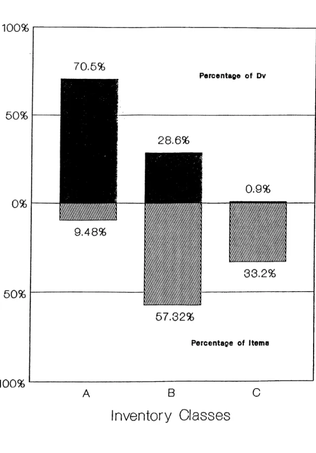
2. PERCENTAGES OF DV AND ITEMS OF EACH CLASS .. 36
1- INTRODUCTION
1.1. THE INVENTORY CONCEPT
Inventories represent stock of goods that are held for a
short term before being converted into sales liras.
They are one of the most active elements of business
operations, and appear on the financial statem e n t s of the
firms. They have a two-way effect on the financial position
of the firm. On one hand, they are assets and therefore
represent stored value that, when sold, will gener a t e revenue
and profit. On the other hand, inventories are usually a
major investment and financed by equity and debt. Therefore,
inventory levels directly affect the return on investment,
which represents the ratio of profit and the average
investment (or level of assets). Return is reduced by the
cost of capital while investment is increased by inventory.
Thus, u n necessarily high inventory levels have a double
negative impact on the return on investment.
Current ratio, the ratio of current assets to current
liabilities, which is the most commonly used measure of
liquidity, is also hi.ghly affected by inventory level changes
(7). Since inventories are classified as one of the current
assets of an o r g a n i s a t i o n , a reduction in their level lowers
assets relative to liabilities. However, the funds freed by
a reduction in inventories normally would be used to acquire
other types of assets or to reduce liabilities. Such actions
In the past, "inventories were considered by merchants,
producers, and policy makers, primarily as a measure of
w e a l t h - "(7). At the beginning of this century, an increased
emphasis was put on the liquidity of assets, such as
inventories, until fast asset turnover became a goal to be
pursued in many o r g a n i s a t i o n s . But in 1970's high inflation
rates, which became common in all world economies, altered
the spending patterns of individuals, companies, and
governments, and caused a tendency towards inventory
increases- Today, most managers recognize the importance of
balancing the advantages and d is a d v a n t a g e s of carrying
inventories- This recognition causes the need for proper
inventory control systems which will minim i z e the cost
incurred in the inventory system, attaining at the same time
the customer service level specified by the com p a n y policies- These two o b j ectives are generally in opposition- High levels of customer service lead to high costs, and low costs usually
are accompanied by low levels of customer service.
Consequently, most inventory decisions are trade-offs between
cost and customer service level (9). The problem is to
achieve a balance with stocking decisions, avoiding both
overstocking and understocking, neither u n n e c e s s a r i 1y tieing
up funds nor causing late deliveries, lost sales and
Inventories are nonpr o d u c t i v e assets which earn no return and
which are subject to loss, pilferage, obsolescence, and
taxes. The main reason for holding inventories is that they
cover discont i n u i t i e s in the supply-demand re 1a t i o n s h i p . In that sense they serve a number of important functions:
1) Inventories are kept on the shelf to satisfy anticipated,
but variable customer demand. The exact demand pattern is not
known with certainty, and products are therefore stocked to
cover the uncertainty involved.
2) Firms that experience seasonal patterns in demand, often
build up inventories during off season periods in order to
meet overly high requirements that exist during certain
periods. This demand pattern results in an inventory buildup
followed by a rapid inventory depletion.
3) Inventory may be stockpiled in anticipation of supply
disruptions, such as weather, strikes or problems with a
s u p p l i e r .
1.2. FUNCTIONS OF INVENTORY
4) Delayed d e l iveries and unexpected increases in demand
increase the risk of shortages. This risk can be reduced by
holding safety stocks, which are stocks in excess of
anticipated demand. The safety stock inventory level is a
stock-outs that can be tolerated.
5) In order to minimize the order costs and/or to take
advantage of price breaks or quantity discounts or meet the
suppliers' minimum order r e q u i r e m e n t s , it may be necessary to buy quantities that exceed immediate usage r e q u i r e m e n t s
-6) At times of price increase expectations, purchases are
realized earlier in order to make savings and higher profits
in future.
7) In order to allow full loads or consolidation of shipments and more efficient use of containers, it may be more feasible to buy in larger quantities, which result in i n v e n t o r i e s .(9)
In order to make the best use of these functions of
inventories, managers need decision and control systems. This study deals with the utilization of inventory control methods as a management t o o l .
The thesis is based on an application made in a retail store
that sells building and construction materials. The purpose
is to practice the application of ABC inventory
classification method. This purpose is matched with the needs of that store towards easing and solving the problems related with managing the great numbers of inventory units. There are nearly 3000 units to control and the only control system used
by the store is the physical counting of the items once a
year. Since there is no continuous control system, and so no
u p - to-date inventory data, store management has difficulties
in making decisions on allocating time and investment on each
item. Currently, such decisions are made on judgemental
basis, depending on their past experiences. This is a very
time consuming task, and makes it impossible to plan the
future and improve the business.
1.3. PURPOSE OF THE THESIS
The owners of this store are at the point of deciding on
’’computerizing the m a n a g e m e n t ” and especially the inventory
control mechanism. At this stage, the current study
concentrates on the means of system-automation feasibility-
In fact, this study c ontains the first stage of implementing
an inventory control system, but as it is intended to help
management decide on such an issue, it is believed to be
sufficient. Extending the content of this effort will be
feasible only in case of approval from the management. In
c 1a 5 5 i f i c a t i o n , and aiding the store management in their decision making regarding the inventory issues.
1.4. BACKGR O U N D OF THE FIRM
The firm subject to the application of this study is a retail
store in the field of construction materials. It was founded
in 1964, as "Ozdemir Duru ve Ortaklari Koll. S t i .", in
Kadikoy, İ s t a n b u l .
In sixties, the construction sector was attractive for
traders, and the competition was not treathening. The firm
made a good start, and formed strong relations with the local
construction firms. The rapid growth in sales and profits
enabled the firm to move to a bigger (current) store
location. The name was changed to " O zd e mi rl e r“ in 1970.
The situation changed in seventies. The construction sector
was in recession, and the market was influenced by inflation.
Another factor contributing to the unatt r a c t i v e n e s s of the
business in 70s was the high competition. Big construction
firms segment was captured by the w holesaler firms founded by construction materials m a n u f a c t u r e r s .
Changing characte r i s t i c s of the market influenced Ozdemirler,
A c c o r d i n g 1y , the firm faced decreases in their sales volume,
and profits. Rather than adapting to the environment,
Ozdemirler tried reducing the general expenditures of the
store, and this caused them to fall behind the competition.
Their new market segment is the local households- The
products appealing to that segment certainly are different
from the former segment of construction firms. However,
□zdemirler has not changed the inventory profile which had
been its differential advantage since the beginning. They
have been carrying 3000 different items, but they can not use
this advantage effectively, due to lack of control over the
inven t o r y .
1.5. OUTLINE OF THE THESIS
This thesis consists of two main parts; theory and
application- In the second chapter, the physical control
techniques are examined. Short and long-term objectives of
inventory control, and functions necessary for an effective
control system are explained and some of the prominent
techniques are cited. Function of ABC inventory
c 1assification - as a base for the control techniques - is
described, and the steps to be followed in classifying the
Third chapter explains the application of ABC c 1assification
to Ozdemirler. The procedure followed in sampling, data
collection, and c 1asification is explained and the results
are e v a 1u a t e d .
The last chapter describes implications of the application
study results, and the further steps that should be taken by
the firm.
2. INVENTORY CONTROL TECHNIQUES
2.1 OBJECTIVES OF INVENTORY CONTROL
Companies attempt to achieve a proper balance between the
benefits of carrying large inventories and the benefits
obtained by reducing inventories to a very low level. The
difficulties associated with attaining this balance on a
solely judgemental basis, lead the management of the firms to
apply "scientific inventory control systems". The long
range objective of any e f f e ctive inventory control system is
to increase the total return on total investment employed by
the company. Some of the short term objectives are :
1) Keeping out~of-stoek con d i t i o n s at a level as low as
p r a c t i c a 1 .
2) Minimizing the costs of carrying and ordering.
3) Maintaining a turnover rate of stocks commensurate with
the level of sales activity. (6).
Furthermore, there will be many additional immediate
objectives which will be important to management at the
particular time. The goal should be to satisfy the maximum
number of the specific objectives as well as the general
There are many factors which must be considered when establishing stock levels. Some of these factors are:
1) The demand for the inventory items must be determined.
This may be established from historical records, or it may be
based on sales forecasts if they are available. The
anticipated demand must allow for fluctuations and must be
frequently modified. A simple inventory system is best
utilized when inventory movement is relatively steady, and
when large random fluctuations are the exceptions. It is
important to review demand rates periodically and adjust the
inventory levels.
2) The lead time for the item must be determined. Lead time
is defined as the time period between the order of an item
and the moment it is placed in stock for use. It includes
ordering lead time as well as vendor production lead time-
Like demand, lead times are not always exactly predictible,
and, therefore, some allowance for variability must be made.
3) Storage facilities: the availability of storage
facilities, or the lack of them, will influence decisions
regarding inventory levels.
4) Another influence on inventory levels is price. Low value
items might be purchased in large quantities taking advantage
of quantity discounts, while higher value items might be
2.2. BASIS FOR INVENTORY DECISIONS
5) Carrying, ordering and shortage costs are other factors
that must be considered in establishing inventory levels.
Carrying (holding) costs include interest, insurance, taxes,
depreciation, obsolescence, deterioration, spoilage,
pilferage, breakage and storage costs. Carrying costs also
include opportunity costs associated with having funds tied
up in inventory that could be used elsewhere. Ordering costs
are the costs associated with ordering and receiving
inventory. They include determining how much is needed,
typing up invoices, inspecting goods upon arrival for quality
and quantity, and moving the goods to temporary
storage. Shortage costs result when demand exceeds the supply
of inventory on hand. The costs can include the opportunity
cost of not making a sale, loss of customer goodwill,
lateness charges, and similar costs. (7).
6) Frequency of engineering changes or the danger of
obsolescence: In industries where technological changes are
rapid or where style changes usually occur, a big risk is
taken when high levels of inventories are maintained.
In the next section as we examine the physical inventory
control systems, we will assume that the demand, lead time
and the costs are known or estimated, so that we can base our inventory level decisions accordingly.
purchased more frequently in smaller
There are numerous systems being used by organizations to
control their inventories. In some o r g a ni za ti o ns — due to the
characteristics of the inventory items— combinations of
several systems may be used together. The most common
inventory control systems are :
1) Min~MaX System : This system involves continuous review
of the inventory. A replenishment is made whenever the
inventory position drops to the reorder point. A maximum
level of inventory which demand will normally not exceed, and a minimum level which is the margin of safety deemed necessary
to prevent out-of-stock c o n ditions from arising is
established. When the minimum level is reached, an order is
pi a c e d . (6).
2.3. INVENTORY CONTROL SYSTEMS
2) Two-Bin System : In this system the stock of each item is
seperated into two piles in such a way that one pile contains
enough stock to satisfy the demand, and the other pile
contains the safety level. When the first pile is finished,
the replenishment order is made, and the stock in the second
pile is used to cover the demand during lead time. The two-
bin system reduces the amount of record keeping, and also
makes it u n n ecessary to take physical counts, since an
automatic reorder point has been set up. "One disadvantage of
the system appears to occur when a single demand is bigger
than the fixed reorder quantity. In such cases, one should
order integer multiples of preset order quantity in order to bring the stock level above the safety stock l e ve l .” (1)
3) Order Cycling System : In this system the quantities on
hand of each item is reviewed periodically by making physical counts. The time periods between each count differs depending
on the type of items. At each review period, orders are
placed to bring stocks up to predetermined levels. If the
demand and the lead times are known with certainty, the
amount to be ordered at each review period and the inventory
level can be determined by the length of the ordering cycle.
But as soon as uncertainty is introduced, safety allowances
for unpredictable variations in demand or lead time must be
calculated. The greater the variability in demand and the
longer the lead time and variability in such lead time, the
greater must be these safety allowances. (6).
An advantage of this system is that orders for many items
occur at the same time and there can be savings in processing
and orders. The d i s a d v antages of the system are the lack of
control between reviews, the need to protect against
shortages between review periods by carrying extra stock, and
the need to make a decision on order quantities at each
r e v i e w .
On 1ine Inyen tory Con t r o 1 System : In case of a
computerized inventory control system, every transaction of
the stock items are recorded. Whenever an item is removed
from inventory^ the date of removal, quantity, material
requisition number are recorded, and the new balance on hand
is calculated. Such a continious record keeping procedure
keeps the inventory control up-to-date every moment. The
d ifficulty of recording each item, especially in multi-item
inventories, usually leads management to make distinctions
between the items with respect to their annua 1- u s a g e - v a 1u e s .
This generally leads to a policy of keeping on-line control
of the higher value items while utilizing the other
predescribed systems for other
items-In order to decide on which items to be controlled by which
system, ABC inventory c 1assification is the most commonly
used method. "ABC inventory c 1assification is a tool of
management for focusing attention on and apply effort in the
area that will give the greatest r e s u 1t s ."(7).
2.4. ABC INVENTORY CLASSIFICATION
In most businesses, a relatively small number of inventory
items account for a relatively large percent of the total
inventory value. By transferring available control effort
from low-value to high-value items, the control effort will
result in maximizing the degree of control over the total
inventory. The ABC inventory c 1assification system divides
the items into categories, and suggests the proper degree of
control for each category of items. In doing that, the
criterion used is the '*annua 1-ueage-va 1 u e " , which is
calculated by multiplying the quantity demanded in a year
(past or forecasted) (D), by the unit cost (v) of the item.
The steps to be followed in classifying the items are as
f o i l o w s :
1) Obtain the price per unit for each manufactured or
purchased item, (v)
2) Obtain the demand in units for each item for the past
year, or from a forecast for some future period of time. (D)
3) Calculate the product of the price per unit (v), and the
usage for the item (D). This will yield the a n n u a 1-usage-
value, which is the value of the item going into the
company's operations over the period.
Arrange the items in the order of decreasing a n n u a 1-usage- v a 1u e .
5) Convert these values into percentages by expressing the
value of each item as a percent of the total value of all
i terns.
6) Roughly divide the list of values into three groups,
namely, A, high-value, B, medium-value, and C, low-value
i terns. (6) .
In making that division, a graph with y-axis as "cumulative
percentage of total annual usage", and x-axis as "percentage
of total number of s.k.u.(stock keeping unit)" can be used.
The resulting graph (Figure 1) makes it easier to divide the
inventory, since the two points where the slope of the curve
changes s i g n i f i c an 1 1y , reveal the annua 1- u s a g e - v a 1ue breaks.
Due to the lack of strict rules, the division is determined
by applying judgment, supported with experience.
In most cases, class A items come out to be the first 5 to 10
percent of total s.k.u. However; since, those are the high
value items, they account for nearly 50 percent of total
annual-1ira-usage of the population of items under
c o n s i d e r a t i o n .
The largest number of s.k.u. fall into class B. Usually more
than 50 percent of total s . k .u — that account for most of the
remaining 50 percent of the a nn ua l - 1 i r a - u s a g e — are worthy of
being labelled B items in any inventory. This percentage is
between 10 to 20 7. of the total money tied up.
Class C items make up only a minor part of total inventory
investment. This group consists of the items that remain
after the A and B classes.
2.4-1. CONTROL OF CLASS A ITEMS
This group of items should receive the most "p e rs o no 1i ze d"
attention from management. Routine controls using the
mathematical models is not enough, and the art of management
becomes important in dealing with them.
Silver and Peterson (1985) suggest the following guidelines
for the control of A items:
1) Inventory records should be maintained on a perpetual
(transactions recording) basis, particularly for the more
expensive items. This need not be through the use of a
computer; the relatively small number of A items makes the
use of a manual system quite attractive.
2) Keep top m a n a gement informed. Frequent reports (for
example, monthly) should be prepared for at least a portion
of the A items.
3) Estimate and influence demand. This can be done in three
w a y s :
a) Manual input to forecasts, for example, knowledge of
intentions of important customers.
b) If the demand is of a special planned nature there is no need to carry protection stock. On the other hand,
where the demand occurs without warning, some
protective stock may be appropriate.
c) Seasonal or random fluctuations can sometimes be
reduced by altering price structures, negotiating with customers, smoothing shipments, and so forth.
4) Estimate and influence supply. Negotiations with suppliers
may reduce the average r e p 1enishment lead time, its
variability, or both.
5) Use "conservative initial p r o v i s i o n i n g .“ (7). For class A
items which have very high unit values, and relatively low
demand rates, the initial provisioning decision becomes
particularly necessary. For such items erroneous initial
overstocking (due to overestimating the demand) can be
extremely expensive. Thus, one should be conservative in
initial provisioning
-6) Review decision parameters frequently. Frequent review of
such quantities, as the order points and order quantities is
advisable for A items.
7) Determine precise values of control quantities. Order
quantities of A items should be based on the most exact
analysis p o s s i b l e .
8) "Confront shortages as opposed to setting service levels."
(7). Rather than setting customer service levels and sitting
back, take action to avoid or eliminate the stock-outs
immediately. Associated costs of such actions should be taken into account when determining the safety stock levels. On the
other hand, since A items are replenished frequently, it may be satisfactory to operate with very low safety stock. (7).
2.4.2. CONTROL OF CLASS В ITEMS
This group carries the greatest number of items (about 507. of
total s.k.u.) in the inventory. The total annua 1- u s a g e - v a 1ue
(D v ) of these items are less than of class A items, thus they rate a moderate but significant amount of attention.
When a computer facility for inventory control is available.
Silver and Peterson (1985) (7) suggest that as many s.k.u. as
possible be monitored and controlled by a с от р и ter-based
system. This seems to be highly attractive in the near
future, given the increasing costs of clerical labor and the
potential costs of human error, versus the constantly
decreasing cost of data processing. Having a larger
proportion of s.k.u. on a computer system also has the
advantage of making a larger data bank available for more
effective and timely management reporting and sales analysis.
If the inventory system is not computerized, management can
try to routinize the decision making by use of manual-based
clerical systems. Under such circumstances the fraction of
s.k.u classified as В items should be reduced, and the
fraction of C items be increased to take advantage of the
lower costs of less paperwork and clerical handling.
With or without the computer, the inventory control system of B class items is the " o n - l in e” inventory control system. All transactions will be recorded and the stoek-on-hand data will
be available and up-to-date each moment. There will still be
need for the physical counts, since continuous recording of
many items will cause a high probability of error. Annual
physical counts may help lower the errors in the inventory
records. In computerized systems, the user will be informed
(by the computer) for each item reaching its reorder point,
and as the ordered items arrive, they will be added to the
stock-on-hand, concurrently being subtracted from stock-on-
order . (1 )
2.4.3. CONTROL OF CLASS C ITEMS
Class C items generally have low totals of replenishment,
carrying, and shortage costs. Regardless of the type of
control system used, management cannot achieve sizable
savings on these costs. Therefore, the inventory control of
this group of items should be based on simple procedures,
that keep the control costs per s.k.u. quite low, by way of
keeping the labor and paperwork per item to a minimum.
"In most cases it may be most a p p ropriate to not maintain any
inventory record of a C item, but, instead simply rely on an
a d m i nistrative mechanism for reordering, such as placing an
order when the last box in a bin is opened" (7). If an
inventory record is maintained, it should not require
recording of each transaction. But, for demand estimation,
and order control purposes a record of the dates of
placement, and of receipts of r e p 1enishment orders, can be
kept.
Following inventory control methods can be feasible for class C items:
1) Periodic review with a relatively long interval (order-
eye 1 i n g - s y s t e m )
2) Two-bin-system, which requires continious review but not
a physical stock count nor the updating of the stock
s t a t u s .
Grouping of C items that have a common supplier, may be
helpful-This method may reduce the ordering costs since when
one item in the group needs ordering, several others will be
included in the ordering cost.
3. AN A P P L I CATION : OZDEM I R L E R
Application of inventory c 1assification study was aiming to
examplify the advantages of systematizing the inventory
control effort of the firm and the potential benefits of
continuous control. Since the management of the store felt
the need for changes in their business structure, they
accepted the idea of evaluating the feasibility of inventory
control automation. However, they still were suspicious of
the d i f f i c u l t i e s , and even the impossibilities of such a
change. Therefore, the most difficult part of the study was
to persuade them into accepting the benefits of scientific
m a n a g e m e n t .
3.1. SAMPLE
We limited our c 1assification study to a sample of the total
inventory, because there was the probability of rejection of
our proposal for the new system. Even though our sample
contains only 232 items, they are chosen with care to be able
to reflect the inventory profile of the firm to a great
extent. The selection of the size of the sample was
not based on any criteria other than the judgement of the
store management- The literature on this issue accepts the
intuitive sample size selection (7). Those items that are
totally disregarded by the m anagement are eliminated at the
beginning. Some of the high-value items were also d i s r e g a r d e d , due to our perception of unreliable data.
3.2. DATA COLLECTION
Data on the items were collected from the records of the
firm. They had annual physical count records for each year,
and the purchase invoices. We used 1986 and 1987 inventory
records and 1987 invoices. So, our base year was 1987.
1986 records gave us the b e g i nn in g- i nv en t or y, and 1987
records gave us the e n d i n g-inventory of each item.
Subtracting the beginning from the e n di n g- in v en to r y, and
adding the total purchases made during the year, we obtained
the annual demand of each item (with the assumption that
there was no unsatisfied demand, so that demand was equal to
sales) ( see Tablel - column 3). As the value of the item, we
used the unit cost of the last purchase, and this enabled us
to e valuate them on the same basis. Collecting such data
revealed that, they were recording the members of an item
category in seperated manner, due to the lack of
s t andardization in identification and the counting procedure.
This caused us to search all through the records for each
item, and bring together the ones that are given more than
one name.
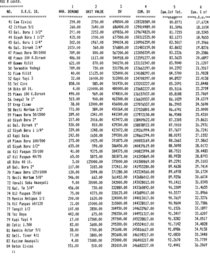
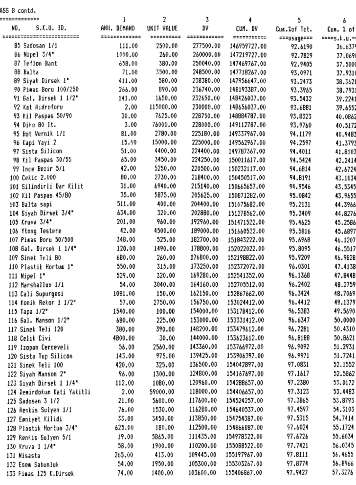
3.3. C L AS S I F I C A T I O N
The first step in c 1assification was to multiply the annual
demand (D) of each item (Table 1-column 1), with its value(v)
(Table 1— column 2), and obtain the annua 1- u s a g e - v a 1ue (D v )
(column 3). We, then, sorted the previous list of items with
respect to annua 1- u s a g e - v a 1ue in descending order; that is
from highest Dv to lowest ( all figures in Table 1 are in
sorted order). Next, we listed the cumulatives of the D v 's
(column 4), and converted those values into percentages
(column 5) in order to express the value of each item as the
percentage of the total value of all items- We also converted
cumulatives of the number of items to percentages of the
total number of items (column 6).
In order to construct the distribution-by-value graph (figure
1), we placed the values in column 5 on y-axis, and column
6 on x-axis, and obtained a concave graph, which helped us in
dividing the inventory into classes (A-B-C), and calculating
the percentages of each class.
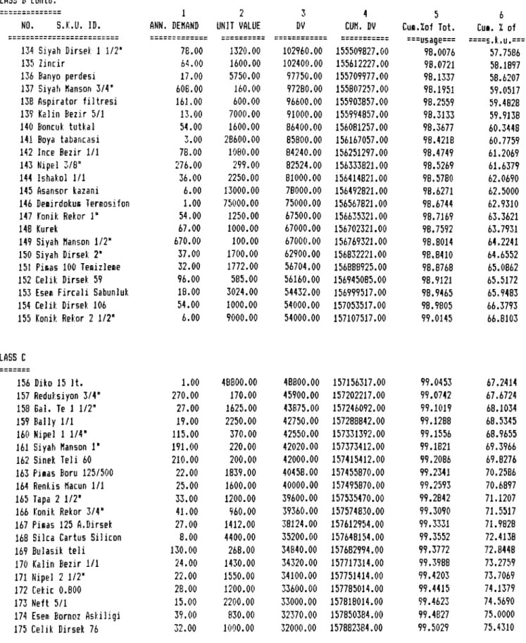
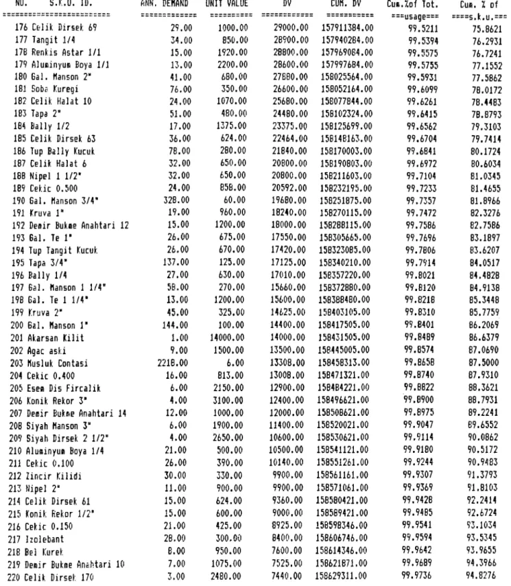
Since there is no specific rule on how to make the division
process, we consulted the store management at that stage.
Their familiarity and experience with the nature of items,
and the already existing examples of ABC c 1assifications in
the literature lead us to make the following c a t e g o r i z a t i o n :
The first 22 of the sample of 232 items were identified as
Class A, the next 133 items as Class B, and the last 77 items as C 1 ass C .
3.4. RESULTS
Such a c 1as5ification yields the following results, and Figure 2.
Classification N o . of s . k . u A 22 s .k .u with Dv > 1,338,930 Percen t s . k . u 9-487. E Dv (TL) 111,794,558 E Dv percent of tot. Dv 70.57. B 133 s .k .u with 1 ,066,240<Dv<54,000 57.327. 45,312,959 28.67. 77 s .k .u with Dv < 48,800 TOTALS 232 33,207. 100.007. 1,563,674 158,671,191 0.97. 100.007.
The figures above show that a very small portion of total
sample, i.e., 9.487., is accounting for 70.57. of total value.
This is class A. The next set of items is class B, containing
133 items, which is 57.327. of all s.k.u, and constitutes
28.67. of total value. The last group is class C, which proves
itself to be very low in total annua 1- u s a g e - v a 1u e . The 77
items in this class, which is 33.27. of all s.k.u, account for only 0.97. of total value.
The division points were also traced on the distribution-by-
value graph and it was observed that they reflect the points
where the slope of the curve changes s i g n i f i c a n t 1y . This
constituted a control of reliability of our c 1a s s i f i c a t i o n .
The increasing concave nature of DBV curve reveals the
different characteristic groups, by its changing slope
a r e a s -(Figure 2)
Class A constitutes the part of the curve where the slope is
high. This is directly related with high cumulative
percentage of Dv of such a small group. Class B items are in
the area of a less steep slope, with a long range. High
number of items in this group (133), compared with 22 of
class A, has much lower percentage of total Dv. This is
reflected on the change of the slope. Class C items are
placed on the last part of the curve, where the slope is
very close to zero. The small percentage of cumulative Dv
causes a very slight increase on the y~axis (0.9’/.).
4. CONCLUSION
The application study was intended to classify the
inventory of Ozdemirler with respect to a n n u a 1- u s a g e ~ v a 1u e ,
in order to set the basis for a feasible inventory control
system. The results revealed that practicing the same level
of control effort on all items was not feasible. While 10
percent of all items was accounting for 71 percent of total
value, 33 percent of items was accounting for only 1 percent.
This result is expected to be effective in convincing the
store management for implementing appropriate control systems
explained in part 2. If the management decides on
с о т р и terizing the control facilities, the range of class В
can be extended to make better use of on-line c o n t r o l . (1).
The sample used in this study contained 232 items. Taking the explained classification procedure as a base, the study needs
to be continued to capture total inventory of the store.
While doing that, data on order costs, reorder points, and
lead times should also be collected or estimated, for
the purposes of improving the inventory decision making
process as well as inventory control.
The resulting table of items may guide the management in
eliminating some of the items from the inventory. Those at
the very end of the list seem to be the candidates for that.
However the management should take into account the needs of
the customers, the service level, and if the items áre complimentary or not.
The classification of the inventory may also help in planning
the placement of the items in the store. Class A and B items
can be placed in heavy traffic parts , while C items can be
stored in the back or the second floor. Groups should not be
divided, when placing with respect to classes; that is, if
members of a group (i-e. water pipes) are seperated in
classification (0.5 inch in class A, 1.25 inch in class B),
they should not be placed seperately since this will cause
bigger problems in control (5).
This classification study, and allocation of appropriate
control effort among classes will certinly improve the
current situation of Ozdemirler. Planning the future will be
possible with the u p - t o-date inventory reports available any
time, and the investment decisions will have a reliable base.
TABLE 1
CLASS A
NO. S.K.U. ID.
1 2
ANN. DEMAND UNIT VALUE 1 Cinto Levha 2 Izocati 6cit. 3 Insaat Çivisi 4 Naylon Branda 5 Su Saati 6 El Arabasi
7 Onduline Oluklu Levh; 8 Stropor 9 Gal. Boru 1/2* 10 talip Kelepçesi 11 Çelik Evye 12 Bos Gidon 13 Silindirli Kilit 14 Aspirator
15 Kutlu Kapak Desenli 16 Yagnurluk 17 Ziftsan 20/1 IB Oluklu Nukavva 19 Gal. Dirsek 1/2* 20 Kisa Cizae 21 Bal. Boru 3/4' 22 Pieas Boru 100/1000 14384.00 890.00 27216.00 5802.00 532.00 296.00 1476.00 109.00 3686.00 4919.00 108.00 633.00 353.00 42.00 287.00 510.00 162.00 2612.00 4341.00 710.00 1310.00 551.00 1600.00 15840.00 490.00 1525.00 15650.00 17500.00 3500.00 40000.00 1128.00 600.00 24000.00 4000.00 6750.00 52920.00 7250.00 3500.00 10000.00 600.00 340.00 1950.00 1045.00 2430.00 3 DV 23014400.00 14097600.00 13335840.00 8846050.00 8325800.00 5180000.00 5173000.00 4360000.00 4157808.00 2951400.00 2592000.00 2532000.00 2382750.00 2222640.00 2080750.00 1785000.00 1620000.00 1567200.00 1475940.00 1384500.00 1368950.00 1333930.00 4 CUM, DV 23014400.00 37112000.00 50447840.00 59295890.00 67621690.00 72801690.00 77974690.00 82334690.00 86492498.00 89443898.00 92035898.00 94567898.00 96950648.00 99173288.00 101254038.00 103039038.00 104659038.00 106226238.00 107702178.00 109086678.00 110455628.00 111794558.00 5 Curı.Zof Tot. ===usage=== 14,5045 23.3892 31.7940 37.3703 42.6175 45.8821 49.1423 51.8901 54.5105 56.3706 58.0042 59.5999 61.1016 62.5024 63.8138 64,9387 65.9597 66.9474 67.8776 68.7501 69.6129 70.4567 Cuı. l of ===s.k.u.=== 0.4310 0.8621 1.2931 1.7241 2.1552 2.5862 3.0172 3.4483 3.8793 4,3103 4.7414 5.1724 5,6034 6.0345 6.4655 6.8966 7.3276 7.7586 8.1897 8.6207 9.0517 9.4828 CLASS B
23 Esen Banyo Dolabi 40.00 26656.00 1066240.00 112860798.00 71.1287 9.9138
24 Ustupu 1414,00 750.00 1060500.00 113921298.00 71.7971 10.3448
25 Terioteknifc 70 İt. 9.00 116000.00 1044000.00 114965298.00 72.4551 10.7759
26 Kutlu Kapak Duz 190.00 5480.00 1041200.00 116006498.00 73.1113 11,2069
27 Bezli Hortuffl 3/4" 1123,00 905.00 1016315.00 117022813.00 73.7518 11.6379 28 Bal. Boru 1* 626,00 1620.00 1014120.00 118036933.00 74.3909 12,0690 29 Cakmakli Terıt. 12.00 78600.00 943200.00 118980133.00 74.9853 12.5000 30 Karshallux 5/1 56.00 16250.00 910000.00 119890133.00 75.5589 12.9310 31 Pifas Boru 125/2000 141.00 6400.00 902400.00 120792533.00 76.1276 13.3621 32 Nipel 1/2" 2121.00 400.00 848400.00 121640933.00 76.6623 13.7931 33 Pilsas Boru 70/1000 655.00 1260.00 825300,00 122466233.00 77,1824 14,2241 34 Siyah Boru 3/4" 980.00 780.00 764400.00 123230633.00 77.6642 14.6552 35 Pisas Boru 70/2000 302.00 2510.00 758020.00 123988653.00 78.1419 15.0862 36 Inegal Te 1 1/4" 600.00 1250.00 750000.00 124738653.00 78.6146 15,5172 37 Renkis Antipas 5/1 94.00 7850.00 737900.00 125476553.00 79.0796 15,9483 38 Gal. Te 1/2" 1308.00 560.00 732480.00 126209033.00 79.5412 16.3793 39 Siyah Boru 1" 632.00 1133.00 716056.00 126925089.00 79.9925 16.8103 40 Elektrik Sayaci 50.00 14100.00 705000.00 127630089.00 80.4368 17.2414 29
TABLE 1 CONTD. CLASS В contd.
1 2 3 4 5 6
NO. S.K.U. ID. ANN. DEHAND UNIT VALUE DV CUH. DV Cum.Kof Tot. Cum. l of
41 Саш Çivisi 254.00 2750.00 698500.00 128328589.00 ===usage=== 80,8771 ====5.k,u.==· 17.6724 42 Ziftsan 5/1 260.00 2640.00 686400.00 129014989.00 81.3096 18.1034 43 Gal. Boru 1 1/2' 273.00 2252.00 659836.00 129674825.00 81.7255 18.5345 44 Siyah Boru 1 1/2" 425.00 1500.00 637500.00 130312325.00 82.1273 18.9655 45 Bal. Boru 1 1/4" 302.00 1967.00 594034.00 130906359.00 82.5017 19.3966 46 Bal. Dirsek 3/4’ 1030.00 560.00 576800.00 131483159,00 82.8652 19.8276 47 Piffias Boru 50/1000 709.00 800.00 567200.00 132050359.00 83.2226 20.2586 4B Pinıas 100 A.Dirsek 486.00 1113.00 540918.00 132591277.00 83.5635 20.6897 47 Бовше Kilit 621.00 870.00 540270.00 133131547.00 83.9040 21,1207 50 Terfflodin Yedeği 709.00 750.00 531750.00 133663297.00 84,2392 21.5517 51 Fian Kilit 40.00 13125.00 525000.00 134188297.00 84.5700 21.9828 52 Kapi Yayi 3 32.00 16000.00 512000.00 134700297.00 84.8927 22.4138 53 Tel Çivi 858.00 585.00 501930.00 135202227.00 85.2091 22.8448 54 Diko 60 İt. 4.00 120000.00 480000.00 135682227.00 85.5116 23.2759 55 Pieas 100 K.Dirsek 490.00 969.00 474810.00 136157037.00 85.8108 23.7069 56 Inegal Te 1" 515.00 900.00 463500.00 136620537.00 86.1029 24.1379 57 Krep Cizee 38.00 12000.00 456000.00 137076537.00 86.3903 24,5690 5B Bezli Hortum 1/2" 771.00 584.00 450264.00 137526801.00 86.6741 25.0000 59 Pieas Boru 50/2000 289.00 1541.00 445349.00 137972150.00 86.9548 25.4310 60 Siyah Boru 2" 217.00 2016.00 437472.00 138409622.00 87.2305 25.8621 61 Bal. Dirsek Г 530.00 810.00 429300.00 138838922.00 87.5010 26.2931 62 Siyah Boru 1 1/4“ 339.00 1248.00 423072.00 139261994.00 87.7677 26.7241 63 Kapi Kolu 242.00 1650.00 399300.00 139661294.00 88.0193 27.1552 64 Pimas Boru 100/500 275.00 1425.00 391875.00 140053169.00 88.2663 27.5862 65 Siyah Boru 1/2" 655.00 590.00 386450.00 140439619.00 88.5098 28,0172 66 Kil Paspas 55/100 41.00 9375.00 384375.00 140823994,00 88.7521 28.4483 67 Kil Paspas 40/70 65.00 5875.00 381875.00 141205869.00 88.9928 28.8793 6B Diko 40 İt. 3.00 125000.00 375000.00 141580869.00 89.2291 29.3103 69 Bal. Boru 2’ 117.00 3183.00 372411,00 141953280.00 89.4638 29.7414 70 Pimas Boru 125/1000 120.00 3094.00 371280.00 142324560.00 89.6978 30.1724 71 Bezli Hortum 5/8" 546.00 662.00 361452.00 142686012.00 89.9256 30.6034
72 Kovali Soba Amasyali 9.00 38000.00 342000.00 143028012.00 90.1411 31.0345
73 Bal. Te 3/4" 456.00 730.00 332880.00 143360892,00 90.3509 31,4655 74 Kil Paspas 35/60 75.00 4375.00 328125.00 143689017.00 90.5577 31.8966 75 Renkis Antipas 1/1 200.00 1620.00 324000.00 144013017.00 90.7619 32.3276 76 Kil Paspas 60/120 21.00 15000.00 315000.00 144328017.00 90,9604 32,7586 77 Tangit 1/2 107.00 2850.00 304950.00 144632967.00 91.1526 33.1897 7B Toz Boya 442.00 675.00 298350.00 144931317.00 91.3407 33.6207 79 Kapi Yayi 4 17.00 17500.00 297500.00 145228817.00 91.5282 34,0517 Ѳ0 Cekic 1.500 82.00 3600.00 295200.00 145524017.00 91.7142 34.4828 81 Renkis Astar 5/1 38.00 7700.00 292600.00 145816617.00 91.8986 34.9138 82 Seli. Tiner 4/1 77.00 3800.00 292600.00 146109217,00 92.0830 35,3448 83 Kuzine Amasyali 4.00 73000.00 292000.00 146401217.00 92.2670 35.7759 84 Beton Çivisi 551.00 510.00 281010.00 146682227.00 92.4441 36.2069 30