On stock rationing policies for continuous review inventory systems

(1)

ON STOCK RATIONING POLICIES FOR CONTINUOUS REVIEW INVENTORY SYSTEMS

A THESIS

SUBMITTED TO THE DEPARTMENT OF INDUSTRIAL ENGINEERING

AND THE INSTITUTE OF ENGINEERING AND SCIENCES OF BILKENT UNIVERSITY

IN PARTIAL FULFILLMENT OF THE REQUIREMENTS FOR THE DEGREE OF

MASTER OF SCIENCE

By Önder Bulut

(2)

I certify that I have read this thesis and that in my opinion it is fully adequate, in scope and in quality, as a thesis for the degree of Master of Science.

Asst. Prof. M. Murat Fadıloğlu (Advisor)

Prof. Nesim Erkip

Asst. Prof. Osman Alp

Approved for the Institute of Engineering and Sciences:

Prof. Mehmet Baray

(3)

iii

ABSTRACT

ON STOCK RATIONING POLICIES FOR CONTINUOUS REVIEW INVENTORY SYSTEMS

Önder Bulut

M.S. in Industrial Engineering Supervisor: Asst. Prof. M. Murat Fadıloğlu

July 2005

Rationing is an inventory policy that allows prioritization of different demand classes. In this thesis, we analyze the stock rationing policies for continuous review systems. We clarify some of the ambiguities present in the current literature. Then, we propose a new method for the exact analysis of lot-for-lot inventory systems with backorders under rationing policy. We show that if such an inventory system is sampled at multiples of supply leadtime, the state of the system evolves according to a Markov chain. We provide a recursive procedure to generate the transition probabilities of the embedded Markov chain. It is possible to obtain the steady-state probabilities of interest with desired accuracy by considering a truncated version of the chain. Finally, we propose a dynamic rationing policy, which makes use of the information on the status of the outstanding replenishment orders. We conduct a simulation study to evaluate the performance of the proposed policy.

Keywords: Stochastic inventory models, stock rationing, multiple demand classes, embedded Markov chains, solution of infinite state space Markov chains

(4)

ÖZET

SÜREKLİ GÖZDEN GEÇİRİLEN ENVANTER SİSTEMLERİNDE STOK TAYINLAMA POLİTİKALARI ÜZERİNE

Önder Bulut

Endüstri Mühendisliği, Yüksek Lisans Tez Yöneticisi: Yrd. Doç. M. Murat Fadıloğlu

Temmuz 2005

Stok tayınlama politikaları, farklı talep sınıfları için bir tür öncelik mekanizması oluşturulmasına yarar. Bu tez çalışmasında sürekli gözden geçirilen envanter sistemleri için stok tayınlama politikaları incelenmiştir. Konuyla ilgili şu ana kadar yapılmış önemli çalışmalardaki muğlaklıklar giderildikten sonra ardısmarlamalı bire-bir envanter sisteminde kritik seviye stok tayınlama politikası için kesin analize imkan veren yeni bir yöntem önerilmektedir. Bu yöntemle gömülü bir Markov zinciri tanımlanmakta ve bu zincirinin geçiş olasılıkları bir özyineli prosedürle üretilmektedir. Kalıcı durum olasılıklarının Markov zincirinin bir bölümü kullanılarak istenilen doğrulukta bulunabileceği gösterilmiştir. Son olarak, beklenen siparişlerin ulaşmalarına kalan zaman bilgisini kullanan dinamik bir stok tayınlama politikası önerilmektedir. Önerilen politikanın performans değerlendirilmesi benzetim deneyleri kullanılarak yapılmıştır.

Anahtar sözcükler: Rassal envanter modelleri, stok tayınlama, çoklu talep sınıfları, gömülü Markov zinciri, sonsuz durum uzaylı Markov zincirlerinin çözümü

(5)

v

ACKOWLEDGEMENT

I would like to express my sincere gratitude to my advisor Asst. Prof. M. Murat Fadıloğlu for all the trust and encouragement.

I am indebted to Prof. Nesim Erkip and Asst. Prof. Osman Alp for accepting to read and review this thesis and for their invaluable suggestions

(6)

CONTENTS

1 Introduction ...1

2 Literature Review...7

3 Notes On The Critical Level Policy and Related Literature ...15

3.1 Priority Clearing Mechanism vs. Other Clearing Mechanisms ...17

3.2 Notes on Dekker et al. (1998) and Deshpande et al. (2003) ...20

4 An Embedded Markov Chain Approach...30

4.1 The Embedded Markov Chain...31

4.2 Steady-State Analysis ...41

5 Rationing With Continuous Replenishment Flow ...53

5.1 Performance Evaluation of RCRF With Simulation...59

6 Conclusion...68

(7)

vii

LIST OF FIGURES

3-1: Threshold Clearing Mechanism... 24 5-1: The ratio of the age of an outstanding order and the leadtime for

(8)

LIST OF TABLES

2-1: Stock Rationing Literature ... 14

3-1: Comparison of the class 2 fill rates that are obtained with threshold clearing and priority clearing ... 26

3-2: Comparison of the class 1 fill rates ... 28

4-1: Numerical experiment (S = 6, K = 3, λ1 = 3, λ2 = 2, L = 1)... 51

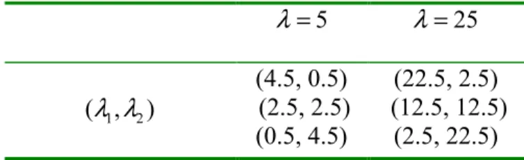
5-1: Arrival rates for the simulation study ... 60

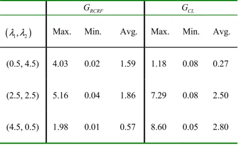
5-2: Percent gain of RCRF over the critical level policy and percent gain of the critical policy over common stock policy when λ = 5... 62

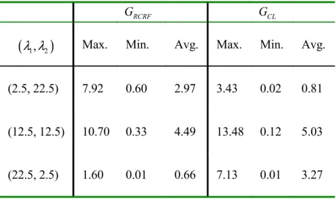
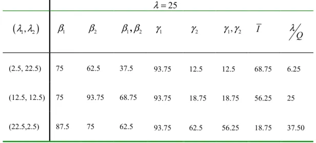
5-3: Percent gain of RCRF over the critical level policy and percent gain of the critical policy over common stock policy when λ = 25... 65

5-4: Percentage of the cases where RCRF provides improvements in cost components when λ = 5 ... 67

5-5: Percentage of the cases where RCRF provides improvements in cost components when λ = 25... 67

(9)

1

C h a p t e r 1

INTRODUCTION

For inventory systems that experience classes of demand for a single item, stock rationing is a well-known tool to differentiate customers. More specifically, stock rationing is an inventory policy that allows prioritization of different demand classes in order to provide different levels of service and to achieve higher operational efficiency. It is possible to maintain high service levels for certain demand classes while keeping inventory costs at bay by providing lower service levels to certain other demand classes. Demand classes are categorized on the basis of their shortage costs. The highest priority class is the one with the largest shortage costs, and the lowest priority has the smallest shortage costs. If there are n demand classes then class 1 has the highest priority, class n has the lowest. In an inventory system with backordering, the ordering of the unit backordering costs is

n

π π

π₁ > ₂ >...> and similarly the ordering of the time dependent backordering costs is πˆ₁ >πˆ₂ >...>πˆ_n.

The systems that have multiple customer classes generating demand for a unit product are frequently observed in real life. For example, in spare parts inventory management, system can experience urgent and critical orders in case of breakdowns that have high shortage costs. On the other hand, the orders due to the planned maintenance activities may be less critical and

(10)

CHAPTER 1 INTRODUCTION

usually have less shortage costs. Again for the spare parts inventory system with multiple end products, same part can be used in many end products that have different importance and criticality. Thus, the demand for any spare part from these end products should be prioritized.

Another example is a two-echelon inventory system consisting of a warehouse and many retailers. In case of stockouts, retailers may place urgent, more critical orders to the warehouse. Again in this setting, if the retailers are located on the basis of regional characteristics of the market area, this situation possibly implies different demand classes and the prioritization of retail orders are beneficial. As another example, in multi- echelon systems the inventory locations in the same echelon can allow shipments between themselves in order to increase the service levels for their direct customers. However, for any inventory location, direct customer orders have superiority over those intershipment orders that are placed by other locations.

Rationing is also a well-known tool in service sectors for customer differentiation. Hotel or airline companies ration their limited capacity according to the priorities of their different customer classes. In this setting, in addition to the rationing decision the key concern is deciding the prices charged to each demand classes. Since the capacity is fixed, in these problems the decisions of when to order and how much to order are irrelevant.

For the systems with multiple demand classes, the most common and easiest strategies are managing individual, separate stock systems for each customer class and managing a common stock pool to serve all the classes without any differentiation. The separate stock strategy permits to assign

(11)

3 different service levels to each customer class, but the positive effect of risk pooling is disregarded. The variability of the demand is higher in this strategy and therefore the whole system has to hold more safety stock to guarantee the desired service levels. On the other hand, common stock strategy uses the pooling effect. Yet this policy causes unnecessary inventory investments for the lower priority classes, because the system provides the highest service level required by the higher priority classes to all demand classes. Inventory rationing policies capture the pooling effect of the demand and in addition to this, they have the flexibility of providing different service levels to different customer classes.

It is possible to define many different kinds of rationing policies, but the mechanism through which any rationing policy is implemented is to stop serving a lower priority class when the inventory on hand inventory drops below a certain threshold level. Under this level only higher priority classes are served and this results in higher service levels for these classes. If there are more than two demand classes, then there is more than a single threshold level. The threshold levels may change dynamically according to the number and the ages of outstanding orders or static threshold levels may be used. The rationing policy with static threshold levels is known as the critical level policy in the literature. For the classic (r, Q) system with critical level rationing, the policy can be defined by the decision variables

(

K,r,Q

)

r

where K

r

represents the vector which consists of (n-1) critical levels. The critical level for the highest priority class is not specified since it is always set to 0. If n = 2 then the policy is

(

K,r,Q

)

.

(12)

structure for the stock rationing problem except for the capacitated make-to-stock production systems. For exponential leadtime Ha (1997a) characterize the optimum policy for lost sales case and Ha (1997b) does for the backordering case. Ha (2000) describes the optimum policy for Erlang distributed leadtime and lost sales case, later Gayon et al. (2005) partially define the optimum policy for the backordering case.

In this thesis, we are interested in traditional inventory systems, which have uncapacitated supply channels. It is obvious that dynamic policies that adjust the critical levels continuously in time by utilizing the information on the number of outstanding orders and their remaining times to arrive, are closer to the unknown optimum structure than the (static) critical level policy. To motivate this fact let us consider an inventory system in which there is an outstanding order that is about to arrive. If the probability of stockout for the higher priority classes in the remaining order arrival time is negligible, then we should choose to satisfy a demand of lower priority class even if the inventory on hand is below the critical level. On the other hand, dynamic decisions considerably complicate the performance evaluation and the optimization of policy parameters. Thus the common practice is to use static threshold levels, i.e. employing critical level policy.

In a backordering environment, stock rationing introduces the problem of making allocation decision of incoming replenishment orders between increasing the stock level and clearing the backorders of different customer classes. The rule that governs this allocation decision is called the clearing mechanism. Without specifying the clearing mechanism, the rationing policy cannot be fully defined for inventory systems with backordering. Consider a system with two demand classes, class1 and class 2, when a replenishment order arrives it is optimal first to clear class 1 backorders due to high

(13)

5 backorder costs of this class. After clearing all class 1 backorders one can give the priority to increasing the stock level up to the critical level. Then if all the order quantity has not been used, s/he can clear the backorders of class 2 starting from the oldest one until using all the remaining order quantity or until the class 2 backorders are depleted. If any units left from the order quantity after all class 2 backorders are filled, those units are added to the inventory to increase the stock level. This clearing mechanism is called priority clearing in the literature. Under priority clearing, inventory level cannot exceed K before clearing all backorders. One possible alternative to priority clearing is, after clearing class 1 backorders one can fulfill the backordered demands of class 2 then increase the stock level. One can come up with many other clearing mechanisms. Some different kinds of clearing mechanisms have already been suggested in the literature mostly due to the fact that exact analysis of stock rationing problem with priority clearing is not available. In a lost sales environment there is no clearing concept.

In this thesis, following a general review of stock rationing literature, we present a detailed analysis of the critical level policy based on our observations in parallel with some notes on the main works in the literature that considered critical level policy and different clearing mechanisms. Then we present our contributions to the literature. The setting we consider is a continuously reviewed single location, and single product inventory system with backordering under rationing. We assume deterministic leadtime, L , and two customer classes that generate Poisson demand arrivals with rates

1

λ and λ₂. We first introduce an Embedded Markov Chain approach to the analysis of (S-1, S) policy under rationing with the priority clearing mechanism. With this approach we are able to obtain the steady state probabilities of the system with desired accuracy by considering a truncated version of an infinite state space Markov chain. These state probabilities

(14)

permit the computation of any long-run performance measure of interest for the system. Finally for the (r, Q) policy, we present a dynamic rationing policy that utilizes the information of the number of outstanding orders and their ages. We conduct a simulation study to quantify the gains through this dynamic policy.

We organized the thesis in six chapters. In the following chapter we discuss the related literature, then in Chapter 3 we present our observations on critical level policy and on some of the important works in the literature. In Chapter 4 we present our embedded Markov chain approach for the (S-1, S) policy under rationing and in Chapter 5 we introduce a dynamic rationing policy. Finally, we provide an overall summary of the study and address future research directions in Chapter 6.

(15)

7

C h a p t e r 2

LITERATURE REVIEW

Similar to other stochastic inventory problems, stock rationing literature can be categorized based on the review policy (continuous/periodic) and on the consequence of shortages (backorders/lost sales). However, in addition to this general categorization research on stock rationing is also classified according to the assumed rationing policy and by the clearing mechanism for the backorders that defines how to handle the arriving replenishment orders. There is also a parallel literature on the production environment, which effectively considers a capacitated replenishment channel.

Rationing models deal with the prioritization of different demand classes and the initial research on this topic were at 1960s, which generally considered the periodic review systems. Veinott (1965) is the first who analyze a periodic review setting with zero leadtime and backordering. He introduces the concept of critical levels as a rationing policy for multiple demand classes. Topkis (1968) worked on the same model and proved the optimality of time remembering critical level policy for both lost sales and backordering cases. His policy is based on dividing every review period into a finite number of subperiods. By using dynamic programming, he finds a critical level for each subperiod and for each demand class that depends on the time to the next review. Critical level is decreasing with the remaining time to review. For the lost sales case Evans (1968) and for the backordering

(16)

CHAPTER 2 LITERATURE REVIEW

case Kaplan (1969) derive essentially the same results for two demand classes.

Nahmias and Demmy (1981) consider a stationary, fixed critical level policy for two demand classes and derive the expected number of backorders for both types of the customer classes for a single period problem and extended the results to an infinite horizon multiperiod problem with the assumed (s, S) policy and zero lead time. They assume that demand is realized at the end of each period. Moon and Knag (1998) generalize the work of Nahmias and Demmy (1981) by considering multiple critical levels and by presenting a simulation analyses.

Cohen et al. (1989) consider a periodic review (s, S) policy with lost sales and two demand classes. At the end of each period, after the realization of demands, they use the on hand stock to meet the demands of customer classes in the order of priorities.

Frank et al. (2003) analyze a periodic review model with two demand classes, one is stochastic and the other is deterministic. High priority class is the one with deterministic demand. Any unsatisfied stochastic demand is lost. They characterize the complex structure of the optimal policy and propose a much simpler critical level policy for (s, S) type replenishment. They assume that the orders arrive instantaneously and aim to use the rationing to gain from fixed ordering cost instead of saving stock for future deterministic demand.

Atkins and Katircioglu (1995) consider service level requirements for each demand classes and propose a heuristic rationing policy that is hard to implement. They have a periodic review setting with fixed lead time and backordering.

(17)

9 In continuous review setting, multiple demand classes and rationing first analyzed by Nahmias and Demmy (1981). Under a

(

r Q,

)

policy they consider a setting with unit Poisson arrivals, two demand classes, constant leadtime, and full backordering. They assume a critical level rationing policy and at most one outstanding replenishment order. Instead of finding the optimum policy parameters, i.e.

(

K r Q, ,

)

and K stands for the critical level, they focus on deriving the expected number of backorders and fill rates for any given parameter set for both demand classes. Moon and Kang (1998) extend the model of Nahmias and Demmy (1981) by considering compound Poisson demand. They analyze the system with a simulation model.

Deshpande et al. (2003) work on exactly the same problem that Nahmias and Demmy (1981) analyze with the exception that they do not have any restriction on the number of outstanding orders. However, in order to get the analytical results of this more general critical level rationing model they do not use the priority clearing mechanism. To derive the steady state inventory level probabilities and to get the operating characteristics of the system they introduce the threshold clearing mechanism that allows clearing low priority backorders before clearing all class 1 backorders and raising the inventory above the critical level. They provide an algorithm to obtain the optimal policy parameters, which result in the minimum expected cost rate. They compare the performance of the threshold clearing with the performance of priority clearing. For the priority clearing, they obtain the optimum levels via simulation.

Melchiors et al. (2000) analyze the model of Nahmias and Demmy (1981) for the lost sales case by preserving the assumption of at most one outstanding order. They allow the critical level to be above the reorder level

(18)

and observe some situations that this case is optimal. Melchiors (2003) extends this model by considering multiple Poisson demand classes and they propose the restricted time remembering policy. He divides the constant leadtime in subintervals and by considering the remaining lead time of the outstanding order finds the critical levels which are restricted to be constant over the subintervals.

Teunter and Haneveld (1996) also consider a time remembering policy in the continuous review setting for two demand classes and backordering. They determine the set of remaining lead time values (L1, L2…) which imply

to reserve 0,1,2… units of stock for high priority customers, i.e. if the remaining time is less than L1 they do not ration the stock, if it is between L1

and (L1+L2) one item is reserved for the high priority class and so on. They

showed that this policy outperforms the critical level policy.

Dekker et al. (1998) work on a spare parts stocking environment with two demand classes and consider (S-1, S) inventory policy that allows backordering. They state that they do not have any restriction on the number of outstanding orders. For the critical level rationing, without assuming any clearing mechanism they derive the exact fill rate expression for the non-critical demand class and make an approximation for the non-critical class fill rate by conditioning on the time that stock level hits the critical level. Afterwards they consider three different clearing mechanisms including the priority clearing and test their approximation under each of these mechanisms using simulation. They also present another approximation for the service level of the critical class, which accounts the effect of the way that the incoming orders are handled.

(19)

11 policy and critical level rationing. However, they assume generally distributed leadtime, multiple demand classes and lost sales. In lost sales case, there is no discussion about clearing. Using queueing results they derive the state probabilities and operating characteristics of the system. They introduce a numerical solution method for optimization.

Ha (1997a) considers a make-to-stock production system with a single production facility, zero setup cost, multiple demand classes and lost sales. He assumes exponentially distributed production leadtime. His system is a capacitated one and order crossing is not possible. Using a queueing model he shows that lot-for-lot policy is optimal for production decision and the critical level policy is optimal for stock rationing decision. Intuitively, for a memoryless system the elapsed time does not provide any information for the arrival time of the replenishment order. Ha (1997b) analyzes the same setting but he allows backordering. He defines the optimal control policy as a monotone switching curve which says that production decision is based on a based stock policy and rationing decision determined by critical level policy which is decreasing in the number of backorders of the non-critical class. Vericourt (2002) considers the multiple demand class extension of Ha (1997b).

Ha (2000) extends Ha (1997a) to an Erlangian production times. He defines the work storage level concept that keeps track of the number of completed Erlang stages for the items in the system. He proves that a critical work storage level is optimal for both production and stock rationing. With a numerical analysis he shows that the critical level policy performs well for the same setting.

(20)

backordering. Using the work storage level concept, they partially characterize the optimal policy. In addition, when they assume a salvage market without a backorder cost they fully characterize the optimal stock rationing policy.

Kocaga (2004) works on the spare parts service system of a leading semiconductor equipment manufacturer. He considers the same setting of Dekker et al. (1998). However, the non-critical orders allow a fixed demand leadtime to be fulfilled. After deriving the service level expressions for both classes, with a numerical study he shows that significant savings are possible through incorporation of demand leadtimes and rationing.

Arslan et al. (2005) considers a continuous review ( , )r Q policy with multiple demand classes, unit Poisson demands and deterministic leadtime. They assume the critical level rationing and analyze this single location inventory system by constructing an equivalent multi stage serial system. The stages in the serial system are defined as inventory systems that face the external demand of corresponding customer class of the original problem. Each stage also sees internal demands from the lower level stages. By assuming a clearing mechanism that clears the backorders at each stage in the order of occurrence, they derive the state probabilities of the system. However, this clearing mechanism allocates the replenishment quantity fairly between the reserve stock for higher classes and the backorders of lower level classes. Thus, it deviates from the priority clearing. They also provide a heuristic for the optimization and describe how their model can be extended to a multi echelon setting.

Zhao et al. (2005) consider a decentralized dealer network in which each dealer can share its inventory with the others. Each dealer gives the high

(21)

13 priority to its own customers and the low priority to other dealers. They assume the critical level rationing and use the threshold clearing mechanism that Dehpande et al. (2003) propose. They analyze the system by constructing an inventory sharing game.

We conclude the chapter with Table 2.1. It summarizes the stock rationing literature. The literature is classified on the basis of the backordering and lost sales cases. Moreover, the works on the production environment, i.e. capacitated replenishment channel, are also provided.

(22)

CHAPTER 2 LITERATURE REVIEW Table 2.1 Stock Rationing Literature

Periodic review Continuous review Production environment

Backordering

Veinott(1965)

Topkis (1968)

Kaplan (1969)

Nahmias and Demmy (1981)

Moon and Kang (1998)

Atkins and Katircioglu (1995)

Nahmias and Demmy (1981)

Teunter and Haneveld (1996)

Dekker et al. (1998)

Moon and Kang (1998)

Deshpande et al. (2003) Melchiors (2003) Kocaga (2004) Arslan et al. (2005) Zhao et al. (2005) Ha (1997b) Ha (2000) Vericourt (2002) Gayon et al. (2005)

Lost sales Topkis (1968)

Evans (1968)

Cohen et .al (1989)

Melchiors et al. (2000)

Dekker et al. (2002)

(23)

15

C h a p t e r 3

NOTES ON THE CRITICAL

LEVEL POLICY AND RELATED

LITERATURE

In this chapter, we present our observations on the critical level policy with two demand classes and backordering under continuous review. These observations can also be extended easily to multiple demand class systems. We clarify many ambiguities resulting from the literature and position the contributions of Dekker et al (1998) and Deshpande et al. (2003), the two important works in the area.

For the stock rationing problem, even with the exponential lead times, i.e. the simplest setting, there is no work in the literature that characterizes the optimal policy structure. Related literature concentrates on the critical level policy, which assumes static threshold level. Although it is known that critical level policy is not optimal, having a fixed threshold level makes it the easiest policy to analyze and implement. Moreover, in literature there is no agreement on the backorder clearing mechanism to be used within the critical level policy. An important reason for assuming clearing mechanisms other than the priority clearing is to make the analytical analysis possible. However, there is no work that clarifies the connection between the critical level policy and the priority clearing mechanism. Although Deshpande et al.

(24)

CHAPTER 3 NOTES ON THE CRITICAL LEVEL POLICY

(2003) state that they propose a different clearing mechanism because they could not get any analytical results with the priority clearing mechanism, they do not assess the necessity of priority clearing when the critical level policy is used.

We organize this chapter in two sections. In section 3.1, we explain why the priority clearing mechanism should be the natural consequence of the critical level policy. In section 3.2, we discuss different clearing mechanisms considered in the literature and also show that when Q= , the fill rate 1 expressions of Deshpande et al. (2003) turn out to be the expressions given in Dekker et al (1998).

Before proceeding with the sections of the chapter, we provide the following notation:

i

β = P

{

an arriving class i customer is served immediately

}

, i.e. fill rate for class i and i = 1,2.

PC i

β = fill rate for class i when the critical level policy is used with the priority clearing mechanism, i = 1,2.

AC i

β = fill rate for class i when the critical level policy is used with an alternative clearing mechanism, i = 1,2.

i

γ = average backorder time per customer for class i, i = 1,2.

PC i

γ = average backorder time per customer for class i when the critical level policy is used with the priority clearing mechanism, i = 1,2.

(25)

17

AC i

γ = average backorder time per customer for class i when the critical level policy is used with an alternative clearing mechanism, i = 1,2.

[ ]

1 2 1(1 1) 1 2(1 2) 2 ˆ1 1 1 ˆ2 2 2 E TC A hI Q λ λ π β λ π β λ π γ λ π γ λ + = + + − + − + + is the

expected total cost rate whereA is the fixed ordering cost, h is the unit holding cost and I is the average inventory.

In this chapter and also in chapter 5, we use simulation results for comparison and performance evaluation purposes. The simulation runs are controlled by the total number of arrivals. We run the simulation until 500,000 total arrivals in order to observe the steady state behaviors of the policies. To verify the accuracy of our simulation, we simulate the critical level policy with the following parameter set;

1 2

5, 1, 3, 3, 2, 1

r= Q= K = λ = λ = L= where L is the leadtime. With the significance level 0.05 and 10 replications, for the fill rate for class 1 we obtained a confidence interval (0.92024, 0.920455) and for the fill rate for class 2 we obtained (0.124471, 0.124742). These confidence intervals are small enough to allow us to use the average of 10 replications for each case.

3.1 The Priority Clearing Mechanism vs. Other Clearing Mechanisms It is possible to define many different clearing mechanisms under the critical level policy. Each policy results in different service levels and expected cost rate due to allocating the order quantity in different ways between increasing the stock level and clearing the backorders of different customer classes. However, the critical level policy provides service to class 2 when the on hand stock is above K and reserves all the stock below K for class 1 customers. Thus, we think that the natural clearing mechanism of the critical

(26)

level policy should be the one that postpones the clearance of class 2 backorders until the on hand inventory reaches K , i.e. until filling the reserve stock of class 1 customers. This clearing mechanism exactly corresponds to the priority clearing. Hence, to make it a well-defined policy, the critical level policy should be defined with the priority clearing mechanism. With any other clearing mechanism, K does not really corresponds to a threshold level under which all the stock reserved for class 1.

We verify the idea mentioned above by considering the effects of clearing mechanisms on the service levels, which are the performance measures of the system, for any fixed set of input policy parameters. It is obvious that upon arrival of replenishment order, the system should first clear class 1, high priority, backorders if there is any, because the time dependent backorder cost of class 1 is higher, that is πˆ₁ >πˆ₂. After the clearance of class 1 backorders, if the order quantity is not depleted, one can choose to clear some class 2 backorders before inventory level reaches K or s/he can first choose to increase the stock level up to K and then clear class 2 backorders. The latter one corresponds to the priority clearing mechanism. If any class 2 backorder is cleared before increasing the stock level up to K , let us call it alternative clearing, the resulting fill rate for class 1, β₁AC, is less than _β₁PC

. This is so because when the priority is given to clearing some or all class 2 backorders, the remaining order quantity may not be enough to increase the inventory up to K . Therefore, compared to the priority clearing, the number of future class 1 demands that finds the system in stockout increases.

(27)

19 backorders before the inventory hits K does not provide any increase in the fill rate for class 2, i.e. β₂AC =β₂PC. This is so because fill rate gives the ratio of customers that are served immediately when they arrive. Under the critical level policy, class 2 arrivals are satisfied when the on hand stock level is between K and (r+Q). Therefore, not only the priority clearing mechanism, any mechanism that requires the clearing of all backorders before increasing the stock level above K results in a class 2 fill rate same asβ₂PC, i.e. the fill rate for class 2 is independent from the clearing mechanism if the stock level increases above K after the clearance of all backorders. These kinds of policies fully allocate the on hand inventory above K to the future arrivals of both classes.

Deviating from the priority clearing mechanism and using an alternative clearing provides some decrease in the total backorder time of class 2 demands. Giving priority to clear some class 2 backorders decreases average backorder time for class 2, i.e. γ₂AC <γ₂PC. However, as we discussed above, compared to the priority clearing, such a clearing mechanism decreases the fill rate for class 1. Thus, there are more backorders from class 1 and so average backorder time for class 1 increases, i.e. γ₁AC >γ₁PC. Increasing average backorder time for class 1 is not rational because πˆ₁ >πˆ₂. Therefore, from the perspective of service levels, the fill rates and the average backorder times, priority clearing should be the natural consequence of critical level policy.

(28)

3.2 Notes on Dekker et al. (1998) and Deshpande et al. (2003)

Nahmias and Demmy (1981) work on the critical level policy for continuous review systems with backordering for the first time in the literature. They assume Poisson arrivals of two demand classes, deterministic leadtime and at most one outstanding replenishment order. The two most important works that generalize the setting of Nahmias and Demmy (1981) are Dekker et al (1998) and Deshpande et al. (2003). Without having any restriction on the number of outstanding orders, Dekker et al (1998) analyze the

(

K S, −1,S

)

policy and Deshpande et al. (2003) consider the more general

(

K r Q, ,

)

policy. However, there are some ambiguities in these works. To point out those ambiguities and to set the connection between these two works we present a deeper analysis in this section.

For the

(

K S, −1,S

)

policy, i.e. the order quantity Q is 1, Dekker et al. (1998) discuss three clearing mechanisms including the priority clearing after deriving expressions for the fill ratesβ₁ andβ₂. Similar to the priority clearing, the other two mechanisms that Dekker et al. (1998) suggest also use the arriving order quantity to clear the oldest class 1 backorder first. However, if there is no class 1 backorder and the stock level is below K, one of the mechanisms gives the priority to clearing the oldest class 2 backorder instead of increasing the stock level. But the other mechanism gives the priority to increasing the stock if a class 1 demand triggered the arriving order; otherwise it gives the priority to clear the oldest class 2 backorder. If the stock level is at K , then both of the mechanisms clear the oldest class 2 backorder if there is any, if not, they increase the stock. Thus, as in the case of the priority clearing, the stock level cannot be increased above K before clearing all the backorders. Therefore, all the three mechanisms result in the

(29)

21 same fill rate for class 2 as we discussed in Section 3.1.

The fill rate expression for class 2 that Dekker et al. (1998) provide is the following: 1 2 0 ( , ) S K x p x L β λ − − = =

∑

(3.1)

In (3.1) p x

(

,λL

)

is the Poisson probability of x arrivals in the leadtime, and

1 2

λ =λ +λ

The logic behind equation (3.1) is as follows: We know that the inventory position is at the order-upto-level S for at any time point t . As in the analysis of Hadley and Whitin (1963), to satisfy a class 2 demand that arrives at t+L, the leadtime demand should be at most inventory position at t minus K− . 1

Dekker et al. (1998) get the fill rate expressions without considering any clearing mechanism. They claim that the expression given in equation (3.1) is exact because the fill rate for class 2 is independent of the clearing mechanism. However, we should point out that β₂ also depends on the clearing mechanism. The independence of β₂ only holds for the clearing mechanisms that clear all class 2 backorders before increasing the inventory level above K. The logic behind the equation (3.1) is only valid for the clearing mechanisms that belong to this category. As noted before, the clearing mechanisms of Dekker et al. (1998) all belong to this category. However, it is easy to show that their claim is not true in general by considering a counter example. If we define a mechanism in such a way that we clear the oldest class 2 backorder after the on hand inventory level reaches K+1, then under this clearing the fill rate for class 2 would be

(30)

certainly greater than the expression given in equation (3.1). Because the ratio of the time that the inventory level is above K increases due to the postponement of clearing class 2 backorders. Then, the probability of satisfying an arriving class 2 demand, i.e. β₂, increases.

The expression that Dekker et al. (1998) suggest for the class 1 fill rate is

(

)

1( ) 1 1 1 1 2 0 ₀ [ ( )] 1 ! ! L S K L y i K S K y i e L y y e dy S K i λ λ λ β β λ − − − − − − − = − = + − −

∑ ∫

(3.2)

The logic behind equation (2) is as follows: Class 1 demands are satisfied in the region that class 2 demands are satisfied. In addition, a class 1 demand that arrived a leadtime later than the time the system observed will be filled if there will be at least one stock on hand, i.e. there should be at most K− 1 class 1 demands within the leadtime. Equation (3.2) tries to capture this fact by conditioning on the “hitting time” of the critical level. Dekker et al. (1998) claim that “hitting time” is

(

S−K

)

stage Erlang random variable with parameter λ₁+λ₂.

As Dekker et al. (1998) state that the expression in (3.2) is independent of the clearing mechanism and so it is an approximation of the realized fill rate for class 1. However, there are some other problems related to this approximation. It is true that at any time point the inventory position is S, but rationing decision depends on the on-hand stock level. Therefore, their “hitting time” is not the real hitting time of critical level K if the on hand level is not S at the time when the system is observed. The inventory level hits K after

(

S−K

)

demand arrivals only if it starts at S. Moreover, even though it is not mentioned, the expression in (3.2) assumes that rationing continues until the end of the leadtime once it starts. This means that the

(31)

23 effect of incoming replenishment orders within the leadtime are ignored. Replenishment orders may increase the inventory level above K . Therefore, within the leadtime system may again start to satisfy class 2 demands. No replenishment order arrival within the leadtime is only possible if the inventory level is at S when the system is observed, i.e. no outstanding orders. This is equivalent to at-most-one-order-outstanding assumption although the authors claim the otherwise. Therefore, if the steady state probability of being at level S decreases, the approximation gets worse dramatically. By increasing the traffic rate this situation can be observed.

Before the comparison of the realized fill rate for class 1 and the approximation of Dekker et al. (1998), let us analyze the clearing mechanism and the fill rate expressions of Deshpande et al. (2003). They consider

(

K r Q, ,

)

policy and proposes the threshold clearing mechanism that allow clearing some class 2 backorders before the inventory level reaches to K . Later Deshpande and Ryan (2005) also use the threshold clearing mechanism. Under this mechanism Deshpande et al. (2003) define a clearing position that starts at r+Q when an order is placed. Up to the threshold level K clearing position decreases with the total demand rateλ =λ₁ +λ₂. Then, it continuous decreasing at rateλ₁. When a replenishment order of size Q arrives, the rules to apply the threshold clearing are as follows:

1. Clear all class 1 and class 2 backordered demand that arrived before the clearing position hits K on the basis of FCFS rule.

2. Clear any remaining class 1 backordered demand if possible with the remaining order quantity. Continue to backorder all class 2 demand that arrive after the clearing position hits K .

(32)

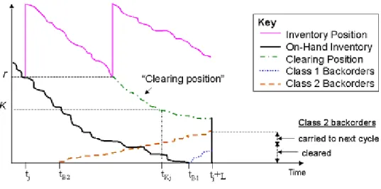
Figure 3.1 summarizes the threshold clearing mechanism for a typical cycle. At time t_j, jthorder is placed. At t_B₂on hand stock hits K and the system start to backorder the class 2 demands. At t_B₁ the on hand stock is depleted. And t_Kjis the time that the clearing position of this specific order hits K . After the completion of the clearing procedure, clearing position and the on hand inventory meet at the same level.

With the threshold clearing mechanism, Deshpande et al. (2003) enables to get the exact steady state characteristics of the system. However, in contrast to the priority clearing, threshold clearing fills some class 2 backlogged demand before filling all class 1 backlogged demands.

FIGURE 3.1 Threshold Clearing Mechanism

As in the case of Figure 3.1, if an order is placed at time t , it will arrive at time t+L. Deshpande et al. (2003) define D(t,t+L)to denote the total demand between the placement and the arrival of the replenishment order. Then, if D(t,t+ )L ≤r+Q−K then all type of backorders are cleared and on hand stock is increased to r+Q−D(t,t+L), which is greater or equal to

(33)

25 K. This is so because, r−D(t,t+L) corresponds to the level after subtracting all satisfied and backordered demands, and this level plus the order quantity Q carried the stock level to at least K . This implies that if the stock level is at or above K , there is no backorders of any type. As in the case of the clearing mechanisms that Dekker et al. (1998) suggested, from the discussion in Section 3.1, the threshold clearing mechanism must result in the same fill rate for class 2 with the priority clearing mechanism. Consequently, the expression in Equation (3.3), which Deshpande et al. (2003) derive under the threshold clearing, must be exactly the same for the priority clearing mechanism.

1 2 1 0 1 ( , ) r Q y K y r x p x L Q β λ + − − = + = =

∑ ∑

(3.3)

Therefore, we can get (3.3) directly without assuming any specific clearing mechanism: As in the analysis of Hadley and Whitin (1963), by conditioning on the inventory position at any time point t , which is uniform on

] , 1

[r+ r+Q , we can get the distribution of on hand stock level by considering the lead time demand. Furthermore, to satisfy a class 2 demand that arrives at t+L, the leadtime demand should be at most inventory position at t minus K-1. This logic is only valid for the clearing mechanisms that our observation is applicable, i.e. β₂ is independent from the clearing mechanism if the stock level increases above K after the clearance of all backorders.

Note that, by assuming Q= and 1 r=S−1, we can get equation (3.1), β₂ of Dekker et al. (1998), from equation (3.3). This is a verification of our observation. Moreover, we test the validity of our observation using simulation results. For 5 cases, which illustrate totally different scenarios by

(34)

considering different arrival rates, leadtimes and

(

K r Q, ,

)

values, Table 3.1 shows the simulation results of β₂ under the priority clearing and the expression given in equation (3.3).

TABLE 3.1 Comparison of the class 2 fill rates that are obtained with threshold clearing and priority clearing

(

λ λ1, 2,L

)

(

K r Q, ,

)

β2 (threshold clearing) 2 β (priority clearing) (0.3, 0.7, 8) (1,10,20) 0.964 0.964 (0.3, 0.7, 8) (5,15,20) 0.978 0.978 (1, 1, 1) (1,1,1) 0.135 0.135 (3, 2, 1) (5, 3, 4) 0.011 0.011 (4, 6, 1) (2, 8, 5) 0.344 0.344

As the last observation, it is important to note that when Q=1, the fill rate expression for class 1 that Deshpande et al. (2003) provides for the threshold clearing turns out to be the approximation of Dekker et al. (1998), which is given in equation (3.2). Interestingly, Dekker et al. (1998) construct the expression in (3.2) without assuming any clearing mechanism, but it gives the exact β₁ under threshold clearing mechanism when Q=1.

When Q=1and r = S−1, β₁ expression of Deshpande et al. (2003) is

1 1 0 1 ( ; ; ) ( , ) x S x S j b x S K K j p x L β α λ ∝ − = = = −

∑∑

− + + (3.4) In (3.4), K j x S j J S x j K K S x j K K S x b + − − − − − + + − = + + − (1 ) )! ( )! ( )! ( ) ; ; (α₁ α₁ α₁ , i.e.

a binomial probability, and 1 1

λ α

λ

= .

(35)

27 probability that the leadtime demand for both classes is at least Sand at least

Kof the leadtime demand is from class 1. But, we can interpret equation (3.4) in a different way.β₁of (3.4) is composed of two parts. First part is the probability that the leadtime demand for both classes is at mostS−K−1. The second part is the probability of S−K total demand within the leadtime, i.e. probability of hitting K within the leadtime, plus at most K-1 class 1 demands in the remaining part of the leadtime. Then at least one unit of inventory is available at the end of the leadtime, i.e. the total demand that decreases the inventory is S− =1

(

S−K

) (

+ K−1

)

. This interpretation of (3.4) is exactly what the equation (3.2) says, which is the class 1 fill rate approximation of Dekker et al. (1998).

As mentioned before, Dekker et al. (1998) derive the approximate β₁

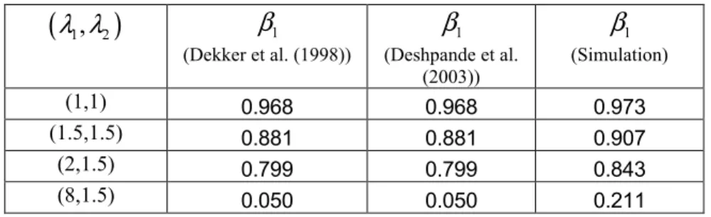
expression, equation (3.2), without assuming any clearing mechanism and Deshpande et al. (2003) work with the threshold clearing mechanism because they are “unable to perform an analysis under the priority clearing”. Moreover, for some parameter sets they test the performance of the threshold clearing mechanism by comparing it with the simulation results of priority clearing. Therefore, for Q=1, we compare their class 1 fill rate expressions, which are equal to each other, with simulation results of the system under the critical level policy with priority clearing mechanism. Table 3.2 demonstrates this comparison for different arrival rates. We choose L= 1 and K = , 1 r= . As we noted before, if the steady state probability of being 4 at level S decreases, the approximation of Dekker et al. (1998) gets worse dramatically. And by increasing the traffic rate this situation can be observed. Table 3.2 illustrates this fact. Moreover it shows that equation (3.2) and (3.4) gives the same results as expected.

(36)

As seen from Table 3.2, for the priority clearing mechanism, equations (3.2) and (3.4) always underestimate the class 1 fill rate. We already stated that the threshold clearing mechanism results in a lower fill rate for class 1 compared to the priority clearing mechanism. However, we can also explain the situation by just considering the approximate fill rate expression for class 1 that is provided by Dekker et al. (1998). Equation (3.2) assumes that the inventory level is at Swhen the system is observed and it decreases with rate

1 2

λ +λ until K , and then decreases with λ₁. Equivalently, this is same as starting at any inventory level and assuming that the replenishment orders clear all the backorders within the leadtime and increases the inventory level up to S. This is a direct application of the logic that is used to derive the steady-state distribution of the inventory level for the

(

S−1,S

)

policy without rationing, i.e. inventory level is S minus the leadtime demand, because if no demand arrives replenishment orders carries the inventory level to S. However, for the

(

K S, −1,S

)

policy, replenishment orders do not clear class 2 backorders and increase the inventory level if it is below K . Increasing the stock instead of clearing a class 2 backorder increases the fill rate for class 1. Therefore, by assuming that all the backorders are cleared within the leadtime, Equation (3.2) underestimates the fill rate for class 1.

TABLE 3.2 Comparison of the class 1 fill rates

(

λ λ1, 2

)

β1 (Dekker et al. (1998)) 1 β (Deshpande et al. (2003)) 1 β (Simulation) (1,1) 0.968 0.968 0.973 (1.5,1.5) 0.881 0.881 0.907 (2,1.5) 0.799 0.799 0.843 (8,1.5) 0.050 0.050 0.211

(37)

29 Before concluding the chapter we summarize our observations:

1. Priority clearing should be the natural clearing mechanism of the critical level policy. Any alternative mechanism negatively affects the service levels for class 1 without any increase in the fill rate for class 2.

2. All clearing mechanisms that clear all backorders before increasing the inventory level above K result in the same fill rate value for class 2.

3. Class 2 fill rate expression of Dekker et al. (1998) is exact only for the clearing mechanisms that clear all backorders before increasing the inventory level above K .

4. The approximation of Dekker et al. (1998) for the fill rate for class 1 is valid if we assume at-most-one-order-outstanding.

5. For Q= , fill rate expressions of Deshpande et al. (2003) turn out to 1 be the expressions that Dekker et al. (1998) provide.

6. For the priority clearing mechanism, class 1 fill rate expressions provided by Deshpande et al. (2003) and Dekker et al. (1998) always underestimate the realized fill rate for class 1.

(38)

C h a p t e r 4

AN EMBEDDED MARKOV

CHAIN APPROACH

In this chapter, we present a new method for the exact analysis of continuous-review lot-per-lot inventory systems with backordering under the critical level rationing policy on two priority classes. This method is based on the observation that the state of the inventory system sampled at multiples of the supply leadtime evolves according to a Markov chain. Our analysis yields the steady-state distribution for the inventory system, which can be used to obtain any long-run performance measure. An exact steady-state analysis for the inventory system was not available up to this point.

The one-step transition probabilities of the embedded Markov chain corresponding to the inventory system are generated using a recursive procedure we develop in Section 4.1. This procedure is based on four recursion equations that are valid in different regions of the state space of the Markov chain and two equations for the boundaries of the state space. Section 4.2 is devoted to steady-state analysis of the chain. In this section, we show that we can get steady-state probabilities of interest with desired accuracy by considering transition probabilities corresponding to a subset of the state space. The application of this technique is mandatory for our problem since the state space for the embedded Markov chain is infinite. Finally, we demonstrate that the technique converges to acceptable accuracy levels fairly quickly by reporting the results of the technique on an instance

(39)

CHAPTER 4 AN EMBEDDED MARKOV CHAIN APPROACH

31 of the inventory system considered.

4.1. The Embedded Markov Chain

We assume inventory for an item is held and replenished over time in order to keep up with the demand from two customer classes, which occur according to two Poisson processes with rates λ₁and λ₂, accordingly. This means that the total demand also follows a Poisson process with rate

1 2

λ =λ +λ . Any unmet demand is backlogged. The inventory policy is a lot-per-lot

(

S−1,S

)

with the critical level rationing and the priority clearing mechanism.

In the analysis of continuous-review inventory systems, the state of the system is usually selected as the inventory level. But under rationing policy, there may be class 2 backorders when the inventory level is under the support level. Thus, one needs a two-dimensional state-space to keep track of the inventory level and the number of class 2 backorders.

To define the state of the system not in terms of the inventory level, but in terms of the number of outstanding replenishment orders lends itself better to analysis. Therefore, we define the state of the system at time t as

(

X t B t( ), ( )

)

, where X t( ) is the number of outstanding replenishment orders at time t and ( )B t is the number of class 2 backorders at time t. Under a lot-for-lot inventory policy, X t( ) is also equal to the number of demand arrivals of both types in (t−L t, ], since each demand arrival triggers a replenishment order. Notice that the inventory level at time t,

( ) ( ) ( ),

(40)

since demand during (t−L t, ] reduces the inventory level from the inventory position at time t−L, which is S, given that it does not correspond to a class 2 backorder. There is no backorder if the inventory level is above the support level K, since all backorders need to be cleared at the support level, i.e.

( ) 0 ( )

B t = if X t <S−K (4.2)

If the inventory level is at K or lower, only class 2 demands that arrive after the inventory level hits K would be backordered. Even if all the demand arrivals in (t−L t, ] belong to class 2, the maximum number of backorders would be X t( ) (− S−K). Thus,

0≤B t( )≤ X t( ) (− S−K) if X t( )≥S−K (4.3) Conditions (4.2) and (4.3) specify the feasible states and thereby the state space of the embedded Markov chain, while Equation (4.1) specifies the inventory level corresponding to each state of the state space.

Given that we know the state of the system at time t, it is possible to derive the probability that the system reaches a certain state at time t+L. If we derive this probability for all feasible states at time t, and at time t+L, then we obtain an embedded Markov chain for the inventory system. These probabilities are the one-step transition probabilities of the Markov chain. They determine the probabilistic evolution of the inventory system at multiples of leadtime. One should note that the original continuous-time process describing the evolution of the states at any point in time is regenerative. The process regenerates itself every time there is no outstanding replenishment order in the inventory system, i.e., when X t( )= 0 and ( )B t = . Since the underlying continuous-time process is regenerative, 0

(41)

33 the process is ergodic and the limiting distribution of the process exists (See Stidham 1974). When the number of transitions for the embedded Markov chain tends to infinity, the probabilities observed will be the probabilities for the continuous-time process as t→ ∞ . Thereby, the limiting distribution of the embedded Markov chain has to be the same with the underlying continuous-time process, i.e.,

{

}

{

}

lim ( ) , ( ) lim ( ) , ( )

t→∞P X t =x B t =b =n→∞P X nL =x B nL =b .

Thus, the limiting distribution of the embedded Markov chain is sufficient for statistical characterization of the inventory system in the long run.

One can observe that one of our state variables X(t), sampled at multiples of leadtime, evolves itself according to an embedded Markov chain. Moreover, the one-step transition probabilities of this embedded Markov chain are independent of the origin state, i.e.

{

( ) | ( ) 0

}

_{

( , ]

_}

(

)

0,1, 2,... ! L x L L t t L L L L L P X t L x X t x P D x e for x x λ λ − + + = = = = = = (4.4) The evolution of X(t), number of outstanding replenishment orders, is fully independent of the rationing policy. The result stated in (4.4) is the basis of the steady-state analysis of

(

S−1,S

)

inventory systems (see Hadley and Whitin (1963) pages 204-205). A direct implication of (4.4) is that the distribution of X(t) converges to its limiting distribution at t=L. Thus, we are able to decouple one of the dimensions of the two-dimensional chain, and solve it independently. This simplifies our analysis considerably.

(42)

CHAPTER 4 AN EMBEDDED MARKOV CHAIN APPROACH We can express all first step probabilities as

(

)

( )

{

( ) L, L| ( ) 0, 0

}

P X t L+ =x B t L+ =b X t =x B t =b

The probabilities that relate to reaching an inventory level above the support level K can be obtained directly from (4.4) as

(

)

( )

{

0 0

}

{

( , ]

}

(

)

0 0

( ) , 0 | ( ) ,

! for 0 , for all feasible ( , ) pairs,

L x L L t t L L L L L P X t L x B t L X t x B t b P D x e x x S K x b λ λ − + + = + = = = = = = ≤ ≤ − (4.5)

since there will be no backorders at time t+L.

One needs considerably more effort in order to obtain other one-step transition probabilities. Since we know the distribution of X(t+L) and the fact that the distribution is independent of X(t) and B(t), we can use this for our objective in

(

)

( )

{

}

(

)

( )

{

}

(

)

0 0 0 0 0 ( ) , | ( ) , | ( ) , ( ) , ! L L L L x L L L x L P X t L x B t L b X t x B t b L P B t L b X t L x X t x B t b e x λ λ ∞ − = + = + = = = = + = + = = =

∑

. (4.6)

Thus, we need to compute

(

)

( )

{

L| ( ) L, ( ) 0, 0

}

P B t+L =b X t+L =x X t =x B t =b (4.7)

for all feasible state pairs

(

x b₀, ₀

)

and

(

x b_L, _L

)

. This is the probability that there are bL units of backorder at time t+L, given that there are b0 units of

(43)

35 backorder at time t, x0 demand arrival occurs in (t−L t, ], and xL demand

arrivals occurs in ( ,t t+L]. Since arrivals occur according to a Poisson process, the unordered arrival times in (t−L t, ] are x0 independent random

variables with uniform distribution on (t−L t, ] and the unordered arrival times in ( ,t t+L] are xL independent random variables with uniform

distribution on ( ,t t+L]. Each demand arrival in (t−L t, ] triggers a replenishment order that arrives exactly in L units of time. This means that replenishment order arrival times in ( ,t t+L] are x0 independent random

variables with uniform distribution on ( ,t t+L]. Moreover, since demand arrival times in (t−L t, ] and ( ,t t+L] are independent, the xL demand and

the x0 replenishment arrival times in ( ,t t+L] are all independent from each

other.

Since the number of order and replenishment arrivals during ( ,t t+L] is known, it is the order of the replenishment and demand arrivals, and the class of the demand arrivals, which determines the number of backorders reached at time t+L. Unfortunately, it is not possible to obtain a closed form expression for the probability expression (4.7). Yet, it is still possible to compute these probabilities using a recursive procedure. This procedure is based on a related probability expression, which can be expressed as

(

)

(

)

( )

{

| , ' , ' , '

}

for ' L L P B t L b X t L x B t b Y t y Z t z t t t L + = + = = = = ≤ ≤ + (4.8)

where Y(t’) is the number of demand arrivals in ( ',t t+L], and Z(t’) is the number of replenishment arrivals in ( ',t t+L], whose occurrence times are

(44)

all independent and identically distributed on ( ',t t+L]. The reader should note that the probabilities in (4.8) do not depend on t’. This independence is due to fact that once the number of arrivals during ( ',t t+L] is known, the duration of the period does not change anything. We can now express (4.7) in terms of (4.8) as

(

)

(

)

( )

{

}

(

)

(

)

( )

{

}

0 0 0 0 | , , | , ' , ' , ' for ' . L L L L L P B t L b X t L x X t x B t b P B t L b X t L x B t b Y t x Z t x t t t L + = + = = = = + = + = = = = ≤ ≤ + (4.9)

The conditions of the conditional probability (4.8), do not include the number of outstanding replenishment orders at time t’. But, given

(

)

_L,

( )

' ,

( )

'

X t+L =x Y t = y Z t =z, this quantity is readily determined by

( ') ( ) ( ') ( ') _L

X t = X t+L +Z t −Y t =x + − z y (4.10) The logic behind Equation (4.10) can be explained as follows: In order to find the number of outstanding replenishment orders at the end of the period ( ',t t+L], i.e., X t

(

+L

)

, one should add the difference between the number of demand arrivals in ( ',t t+L] (which trigger new replenishment orders) and the number of replenishment arrivals in ( ',t t+L] (which clear the outstanding replenishment orders) to the number of outstanding replenishment orders at the beginning of the period.

The recursive procedure devised to compute the probabilities defined by (4.8) is based on the fact that the probabilities conditioned on the number of arrivals that occur in ( ',t t+L], can be written in terms of the same kind of probabilities conditioned on fewer arrivals during the same period. In order to write these relations, we need to consider what happens next depending on

(45)

37 the nature of the first arrival in ( ',t t+L]. There are three possible events that can take place: a replenishment order arrival, a class 1 demand arrival, and a class 2 demand arrival. Since the arrivals in ( ',t t+L] will be uniformly distributed on ( ',t t+L], the probability that a replenishment order arrives first is the proportion of outstanding replenishments to the total number arrivals, i.e. Z t( ') /

(

Z t( ')+Y t( ')

)

. The complement of this probability,

(

)

( ') / ( ') ( ')

Y t Z t +Y t , is the probability that a demand arrival occurs first. This demand arrival will be of class 1 with probability p₁=λ₁/

(

λ₁+λ₂

)

and will be of class 2 with probability p₂ = −1 p₁.

The effect of this first arrival depends on the number of outstanding replenishment orders at that time as a result of rationing policy. If the number of outstanding replenishment orders is less than S-K, then there is no backorder in the system and a demand arrival does not cause any backorder either, i.e.,

(

)

(

)

( )

{

}

(

)

(

)

( )

{

}

(

)

(

)

( )

{

}

if 0 1, then | , ' 0, ' , ' | , ' 0, ' , ' 1 | , ' 0, ' 1, ' . L L L L L L L x z y S K P B t L b X t L x B t Y t y Z t z z P B t L b X t L x B t Y t y Z t z z y y P B t L b X t L x B t Y t y Z t z z y ≤ + − ≤ − − + = + = = = = = + = + = = = = − + + + = + = = = − = + (4.11)

If the number of outstanding replenishment orders is exactly S-K, again there is no backorder at the system. If a replenishment order arrives first, then the state will move to the region of Equation (4.11). If a class 1 demand