Copyright © 2007 Inderscience Enterprises Ltd.
Climbing depth-bounded discrepancy search for
solving hybrid flow shop problems
Abir Ben Hmida*
Université de Toulouse, LAAS-CNRS,
7 avenue du Colonel Roche, Toulouse, France
Ecole Polytechnique de Tunisie, Unité ROI, La Marsa, Tunisia E-mail: [email protected] *Corresponding author
Marie-José Huguet and Pierre Lopez
Université de Toulouse, LAAS-CNRS,
7 avenue du Colonel Roche, Toulouse, France
E-mail: [email protected] E-mail: [email protected]
Mohamed Haouari
Ecole Polytechnique de Tunisie, Unité ROI, La Marsa, Tunisia Faculty of Business Administration Bilkent University, Ankara, Turkey E-mail: [email protected]
Abstract: This paper investigates how to adapt some discrepancy-based search methods to solve Hybrid Flow Shop (HFS) problems in which each stage consists of several identical machines operating in parallel. The objective is to determine a schedule that minimises the makespan. We present here an adaptation of the Depth-bounded Discrepancy Search (DDS) method to obtain near-optimal solutions with makespan of high quality. This adaptation for the HFS contains no redundancy for the search tree expansion. To improve the solutions of our HFS problem, we propose a local search method, called Climbing Depth-bounded Discrepancy Search (CDDS), which is a hybridisation of two existing discrepancy-based methods: DDS and Climbing Discrepancy Search (CDS). CDDS introduces an intensification process around promising solutions. These methods are tested on benchmark problems. Results show that discrepancy methods give promising results and CDDS method gives the best solutions.
[Received 27 October 2006; Revised 27 February 2007; Accepted 8 March 2007]
Keywords: scheduling; hybrid flow shop; HFS; discrepancy search methods; climbing depth-bounded discrepancy search; CDDS; lower bounds; LBs; heuristics.
Reference to this paper should be made as follows: Ben Hmida, A., Huguet, M-J., Lopez, P. and Haouari, M. (2007) ‘Climbing depth-bounded discrepancy search for solving hybrid flow shop problems’, European J.
Industrial Engineering, Vol. 1, No. 2, pp.223–240.
Biographical notes: Abir Ben Hmida is pursuing her PhD in the University of Tunis El Manar (Tunisia). Currently, she is pursuing her dissertation on scheduling problems with resource flexibility (Hybrid Flow Shop, Flexible Job Shop and Resource-Constrained Project Scheduling). She received her Bachelor’s Degree (2001) from Monastir University, Tunisia and also received her MSc from Tunis El Manar University (2004). Her research interests are in the areas of production planning and scheduling.
Marie-José Huguet is an Assistant Professor in Computer Science at the University of Toulouse (INSA), France. Her research works deal with scheduling problems, constraint propagation and tree search procedures. She teaches in the area of combinatorial optimisation, graphs and algorithms. Pierre Lopez received an MS and a PhD in Control Engineering from the University Paul Sabatier, Toulouse, France. During his Doctoral thesis he developed methods of energy-based reasoning applied to task scheduling. Since 1992, he has held a research position at the ‘Laboratoire d'Analyse et d'Architecture des Systèmes’ of the French Center of Scientific Research (LAAS-CNRS). His research area includes constraint programming and temporal reasoning under resource constraints applied to scheduling problems. Mohamed Haouari is a Professor of Operations Research at the Tunisia Polytechnic School. He received a PhD in Industrial Engineering from the Ecole Centrale de Paris (France). His research interests include the design and analysis of exact and approximate solution procedures for combinatorial optimisation problems, with applications in: scheduling and planning, network design, airline operational planning, vehicle routing and supply chain management.
1 Introduction
In this paper, we consider the Hybrid Flow-Shop (HFS) scheduling problem which can be stated as follows. Consider a set J = {J1, J2, …, JN} of N jobs and a set E = {1, 2, …, L} of L stages, each job is to be processed in the L stages. Solving the HFS problem consists in assigning a specific machine to each operation of each job as well as sequencing all operations assigned to each machine. Machines used at each stage are identical and let M(s) be the number of machines in the stage s. Successive operations of a
job have to be processed serially through the L stages. Job preemption and job splitting are not allowed. The objective is to find a schedule which minimises the maximum completion time, or makespan, defined as the elapsed time from the start of the first operation of the first job at stage 1 to the completion of the last operation of the last job at stage L.
The HFS problem is NP-hard even if it contains two stages and when there is, at least, more than one machine at a stage (Gupta, 1988). Using popular three-field notation (see e.g. Hoogeveen et al., 1996), this problem can be denoted by FL(P)||Cmax.
Detailed reviews of the applications and solution procedures of the HFS problems are provided in Gupta (1992), Kis and Pesch (2005), Lin and Liao (2003) and Moursli and Pochet (2000).
Most of the literature has considered the case of only two stages. In Lin and Liao (2003), authors presented a case study in a two-stage HFS with sequence-dependent setup times and dedicated machines. For more general cases (i.e. with more than two stages), some authors developed a Branch and Bound (B&B) method for optimising makespan, which can be used to find optimal solutions of only small-sized problem instances (Brah and Hunsucker, 1991). Later, this procedure has been improved in Portmann et al. (1992). In this latter study, several heuristics have been developed to compute an initial upper bound and a genetic algorithm improves the value of this upper bound during the search. In order to reduce the search tree, new branching rules are proposed in Vignier (1997). Another B&B procedure for this problem is proposed by Carlier and Néron (2000). They proved that their algorithm is more efficient than previous exact solution procedures.
Different heuristic methods were developed to solve HFS problems. Brah and Loo (1999) expanded five standard flow shop heuristics to the HFS case and evaluated them with respect to Santos et al.’s (1995) Lower Bounds (LBs). Recently, a new heuristic method based on Artificial Immune System (AIS) has been proposed to solve HFS problems (Engin and Döyen, 2004) and proves its efficiency. Results of AIS algorithm have been compared with Carlier and Néron’s LBs.
LBs are developed in the literature which can be used to measure the quality of heuristic solutions when the optimal solution is unknown. Various techniques were proposed for obtaining LBs. In Lee and Vairaktarakis (1994), authors reduce the HFS problem to the classical one and the optimal makespan of the latter one is a LB on the optimal makespan of the original problem. In Linn and Zhang (1999), authors defined LBs based on the single-stage subproblem relaxation. The aggregation of the work yields a very rich class of LBs based on computing the total amount of work on some stages or machines (Guinet et al., 1996). Brah and Hunsucker proposed two bounds for the HFS problem, one based on machines and another based on jobs (Gupta, 1988). Their LBs have been improved, later, by Portmann et al. (1992).
The rest of this paper is organised as follows. Section 2 gives an overview of discrepancy-based search methods. Section 3 presents how to adapt some of these methods to solve the HFS problem and details the LBs used. Section 4 is dedicated to an illustrative example to explain the proposed search methods. In Section 5, evaluations of the proposed methods on usual benchmarks are detailed. Finally, we report some conclusions and open issues to this work.
2 Discrepancy-based search methods
Discrepancy-based methods are tree search methods developed for solving combinatorial problems. These methods consider a branching scheme based on the concept of discrepancy to expand the search tree. This can be viewed as an alternative to the branching scheme used in a Chronological Backtracking method.
The primal method, Limited Discrepancy Search (LDS), is instantiated to generate several variants, among them, Depth-bounded Discrepancy Search (DDS) and Climbing Discrepancy Search (CDS).
2.1 Limited discrepancy search
The objective of LDS proposed by Harvey (1995) is to provide a tree search method for supervising the application of some instantiation heuristics (variable and value ordering). It starts from an initial variable instantiation suggested by a given heuristic and successively explores branches with increasing discrepancies from it, that is, by changing the instantiation of some variables. This number of changes corresponds to the number of discrepancies from the initial instantiation. The method stops when a solution is found (if such a solution does exist) or when an inconsistency is detected (the tree is entirely expanded).
The concept of discrepancy was first introduced for binary variables. In this case, exploring the branch corresponding to the best Boolean value (according a value ordering) involves no discrepancy while exploring the remaining branch implies one discrepancy. It was then adapted to suit to non-binary variables in two ways. The first one considers that choosing the first ranked value (rank 1) leads to 0 discrepancy while choosing all other ranked values implies 1 discrepancy. In the second way, choosing value with rank r implies r − 1 discrepancies.
Dealing with a problem defined over N binary variables, an LDS strategy can be described as shown in Algorithm 1.
Algorithm 1 Limited discrepancy search
k ← 0 -- k is the number of discrepancies kmax ← N -- N is the number of variables
Sref ← Initial_solution() -- Sref is the reference
solution
while No_Solution() and (k < kmax) do
k ← k+1
-- Generate leaves at discrepancy k from Sref -- Stop when a solution is found
Sref’ ← Compute_Leaves(Sref, k)
Sref ← Sref’ end while
In such a primal implementation, the main drawback of LDS is to be too redundant: during the search for solutions with k discrepancies, solutions with 0 to k − 1 discrepancies are revisited. To avoid this, Improved LDS method (ILDS) was proposed by Korf (1996). Another improvement of LDS consists in applying discrepancy first at the top of the tree to correct early mistakes in the instantiation heuristic; this yields the DDS method proposed by Walsh (1997). In the DDS algorithm, the generation of leaves with k discrepancies is limited by a given depth.
All these methods (LDS, ILDS, DDS) lead to a feasible solution, if it exists and are closely connected to an efficient instantiation heuristic. These methods can be improved
by adding local constraint propagation such as Forward Checking (Haralick and Elliot, 1980). After each instantiation, Forward Checking suppresses inconsistent values in the domain of not yet instantiated variables involved in a constraint with the assigned variable.
2.2 Climbing discrepancy search
CDS is a local search method which adapts the notion of discrepancy to find a good solution for combinatorial optimisation problems (Milano and Roli, 2002). It starts from an initial solution suggested by a given heuristic. Then nodes with discrepancy equal to one are explored first, then those at discrepancy equal to 2 and so on. When a leaf with an improved value of the objective function is found, the reference solution is updated, the number of discrepancies is reset to 0 and the process for exploring the neighbourhood is again restarted (see Algorithm 2).
Algorithm 2 Climbing discrepancy search
k ← 0 -- k is the number of discrepancies kmax ← N -- N is the number of variables
Sref ← Initial_Solution() -- Sref is the reference
solution
while (k < kmax) do
k ← k+1
-- Generate leaves at discrepancy k from Sref
Sref’ ← Compute_Leaves(Sref, k)
if Better(Sref’, Sref) then
-- Update the current solution
Sref ← Sref’
k ← 0
end if end while
The aim of CDS strategy is not to find only a feasible solution, but rather a high-quality solution in terms of criterion value. As mentioned by their authors, the CDS method is close to the Variable Neighbourhood Search (VNS) (Hansen and Mladenovic, 2001). VNS starts with an initial solution and iteratively explores neighbourhoods more and more distant from this solution. The exploration of each neighbourhood terminates by returning the best solution it contains. If this solution improves the current one, it becomes the reference solution and the process is restarted. The interest of CDS is that the principle of discrepancy defines neighbourhoods as branches in a search tree. This leads to structure the local search method to restrict redundancies.
2.3 Example
As an example to illustrate the above exploration processes, let us consider a decision problem consisting of three binary variables x1, x2, x3. The value ordering heuristic orders
nodes left to right and, by convention, we consider that we descend the search tree to the left with xi = 0, to the right with xi = 1, ∀ i = 1, 2, 3. A solution is obtained with
the instantiation of the three variables. Initially the reference solution Sref is reached with
the instantiation [x1 x2 x3] = [0 0 0]. The solutions with 1 discrepancy from Sref are those
with one digit of [x1 x2 x3] equal to 1, for example, [0 0 1]. To graphically represent the
discrepancies that are performed to reach a solution (and also to be more homogeneous in the explanation of the different strategies), we associate a black circle to an instantiation which follows the value ordering heuristic whilst an open circle designates a discrepancy. In particular, following this semantics, Sref is then associated to ●●● and the
solution with one discrepancy on x3 is associated to ●●○. Finally, the value of a given
objective function f (suppose a minimisation problem) is associated to a solution.
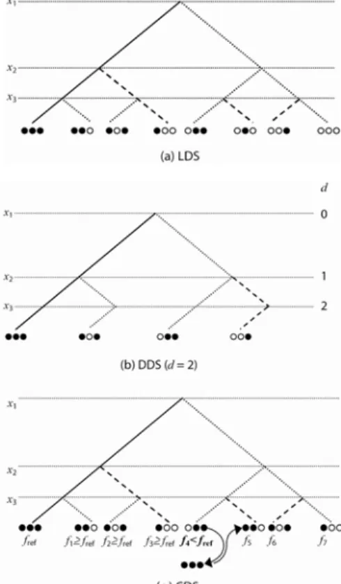
Figure 1 illustrates the search trees obtained using LDS (a), DDS (b) and CDS (c). For all these three methods, the search starts from a reference solution Sref of value fref
obtained with [x1 x2 x3] = [0 0 0]. We see in Figure 1(a) that the eight leaves that are
obtained with LDS correspond to the different solutions that are reachable from ●●●. In Figure 1(b), the tree contains four leaves only since the depth d is fixed at two and thus discrepancies can solely be made over x1 and x2. Figure 1(c) illustrates the search
tree obtained with CDS. The first reached solution from Sref is of value f1 with a
corresponding discrepancy equal to 1. Since f1 is greater than fref, then a second solution
of value f2 is generated. Again, its cost is compared with fref and this process is repeated
until a solution of value f4 having an improved cost is obtained. Thus, f4 becomes the new
reference solution. Therefore, the next solution (of criterion value f5) is only at one
discrepancy from this new reference solution.
3 Discrepancy-based methods to solve the hybrid flow shop problem
3.1 Problem variables and constraints
To solve the HFS problem under study, at each stage, we have to select a job, to allocate a resource for the operation of the selected job and to fix its start time. Since the start time of each operation will be fixed as soon as possible to reduce the makespan, we only consider two kinds of variables: job selection and resource allocation. The values of these two kinds of variables are ordered following a given instantiation heuristic presented below.
At each stage s, we denote by Xs the job selection variables vector and by As the resource allocation variables vector. Thus, s
i
X corresponds to the ith job in the sequence and s
i
A is its affectation value (∀ =i 1,...,N, with N the number of jobs). The domain of
s i
X variable is {J1, J2,…, JN}, ∀ =i 1,...,N and ∀ =s 1,...,L which corresponds to the
choice of job to be scheduled. The values taken by the s i
X variables have to be all different. The s
i
A domains are {1,…, M(s)},∀ =i 1,...,N. Moreover, we consider
precedence constraints between two consecutive operations of the same job and duration constraints for each operation at a given stage.
3.2 Discrepancy for HFS
Despite the fact we have two kinds of variables, we only consider here just one kind of discrepancy: discrepancy on job selection variables. Indeed, our goal is to improve the makespan of our solutions and since all resources are identical, discrepancy on allocation variables cannot improve it. Thus, only the sequence of jobs to be scheduled may have an impact on the total completion time. More precisely, we aim at finding a good job order selection on the first stage. Next, stages 2, …, L are sequenced in turn. Each stage being sequenced using a specified priority rule. Hence a job selection order is defined for stage 1 and then a complete schedule is obtained through propagation. Clearly, an alternative strategy would require defining a specific job order selection for each stage. However, we have performed some preliminary computational experiments and we found that this latter strategy requires very long computer times without yielding significant better solutions.
Therefore, doing a discrepancy consists in selecting another job to be scheduled than the job given by a value ordering heuristic. Job selection variables are N-ary variables. The number of discrepancy is computed as follows: the first value given by the heuristic corresponds to 0 discrepancy, all the other values correspond to 1 discrepancy (see Figure 2).
To obtain solutions of k + 1 discrepancies directly from a solution with k discrepancies (without revisiting solutions with 0,…, k − 1 discrepancies), we consider the last instantiated variable having the kth discrepancy value and we just have to choose a remaining variable for the k + 1th discrepancy value.
At each stage s, the maximum number of discrepancy is N − 1 which leads to develop a tree of N! leaves (all the permutations of jobs are then obtained).
3.3 Instantiation heuristics and propagation
Variable ordering follows a stage-by-stage policy. The exploration strategy firstly consider job selection variable to choose a job, secondly consider resource allocation variable to assign the selected job to a resource.
We have two types of value ordering heuristics: the first one ranks jobs whilst the second one ranks resources.
Type 1: job selection Several priority lists have been used. We first give the priority to the job with the Earliest Start Time (EST) and in case of equality, we consider three alternative rules: Smallest Processing Time (SPT) rule on the first stage Longest Processing Time (LPT) rule on the first stage and Critical Job (CJ) rule. The latter rule gives the priority to the job with the longest total duration.
We also consider all different combinations between these three heuristics. So, we give priority to the job having the EST and, in case of equality, we consider SPT (respectively LPT/CJ) rule on the first stage and LPT or CJ (respectively SPT or CJ/SPT or LPT) in the second and so on. The idea behind these combinations has the aim to mitigate the various configurations of machines.
Type 2: assignment of operations to machines The operation of the job chosen by the heuristic of Type 1, is assigned to the machine such that the operation completes as soon as possible, that is, following an ECT rule. This latter rule is dynamic; the machine with the highest priority depends on the machines previously loaded.
After each instantiation of Type 2, we use a Forward Checking constraint propagation mechanism to update the finishing time of the selected operation and the starting time of the following operation in the job routing. We also maintain the availability date of the chosen resource.
3.4 Proposed discrepancy-based methods
In our problem, the initial leaf (with 0 discrepancy) is a solution since we do not constrain the makespan value. Nevertheless we may use discrepancy principles to expand the tree search for visiting the neighbourhood of this initial solution. The only way to stop this exploration is to fix a limit for the CPU time or to reach a given LB on the makespan. To limit the search tree, one can use the DDS method which considers in priority variables at the top of the tree (job selection at the initial stages).
Thus, we first propose an adaptation of the initial DDS method based on the use of the variable ordering heuristics of types 1 and 2, joined with a computation of LBs at each node according to Portmann et al.’s (1992) rules (see below).
Furthermore, to improve the search we may consider the CDS method which goes from an initial solution to a better one and so on. The idea of applying discrepancies only at the top of the search tree can be also joined with the CDS algorithm to limit the
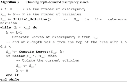
tree search expansion. We have then developed a new strategy called CDDS method. With this new method, one can restrict neighbourhoods to be visited by only using discrepancies on variables at the top of the tree (see Algorithm 3).
Algorithm 3 Climbing depth-bounded discrepancy search
k ← 0 -- k is the number of discrepancy kmax ← N -- N is the number of variables
Sref ← Initial_Solution() -- Sref is the reference solution
while (k < kmax) do
k ← k+1
-- Generate leaves at discrepancy k from Sref
-- and at d-depth value from the top of the tree with 1 ≤ d ≤ k
Sref’← Compute_Leaves(Sref, k)
if Better(Sref’, Sref) then
-- Update the current solution
Sref ← Sref’
k ← 0
end if end while
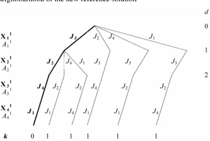
Figure 3 shows the tree obtained by CDDS from the examples depicted in Figure 1(b) and (c).
Figure 3 The CDDS method
We can further enhance the CDDS strategy through the calculation of a LB at each node. So, we have the idea of introducing the LBs developed in Gupta (1988) and improved in Portmann et al. (1992) which can be presented as follows (see also Kis and Pesch (2005) as a survey presentation).
Suppose all jobs are sequenced on stages 1 through L − 1 and a subset Y of jobs is already scheduled at stage s. Let consider Sch(s)(Y) a partial schedule of jobs Y at stage s
Having fixed the schedule of jobs on the first L − 1 stages and that of the jobs in Y at stage s, the average completion time of all jobs at stage s, ACT[Sch(s)(Y)], can be
computed as follows: ( ) ( ) ( ) ( ) 1 ( ) ( ) [Sch ( )] ACT[Sch ( )] s M s s j m j J Y s m s s p C Y Y M M ∈ − = =
∑
+∑
(1)The expression of the maximum completion time of jobs in Y at stage s, MCT[Sch(s)(Y)], is given by ( ) ( ) ( ) 1 MCT Sch ( ) max Sch ( ) s s s m M Y C Y m ≤ ≤ ⎡ ⎤= ⎡ ⎤ ⎢ ⎥ ⎢ ⎥ ⎣ ⎦ ⎣ ⎦ (2)
The machine-based LB, LBM, is defined by
{
}
{
}
( ) ( ') ' 1 ( ) ( ) ( ) ( ) ( ') ' 1 ACT Sch ( ) min LBM Sch ( ) if ACT Sch ( ) MCT Sch ( ) MCT Sch ( ) min otherwise L s s i s s i J Y s s s L s s i s s i Y Y p Y Y Y Y p = + ∈ − = + ∈ ⎧⎪ ⎡ ⎤ + ⎪ ⎢⎣ ⎥⎦ ⎪⎪ ⎪⎪⎪ ⎡ ⎤=⎨ ⎡ ⎤≥ ⎡ ⎤ ⎢ ⎥ ⎢ ⎥ ⎢ ⎥ ⎣ ⎦ ⎪⎪ ⎣ ⎦ ⎣ ⎦ ⎪⎪ ⎡ ⎤ + ⎪ ⎢⎣ ⎥⎦ ⎪⎪⎩∑
∑
(3)The job-based LB, LBJ, is given by
{
}
( ) ( ) ( ) ( ') 1 ' LBJ Sch ( ) min Sch ( ) min s L s s s i i J Y m M s s Y C Y m p ∈ − ≤ ≤ = ⎧ ⎫ ⎪ ⎪ ⎪ ⎪ ⎡ ⎤= ⎡ ⎤ + ⎨ ⎬ ⎢ ⎥ ⎢ ⎥ ⎣ ⎦ ⎣ ⎦ ⎪⎪⎩∑
⎪⎪⎭ (4)Finally, we obtain the composite LB, LBC, which given by
{
}
( ) ( ) ( )
LBC Sch ( )⎣⎡⎢ s ⎤⎥⎦=max LBM Sch ( ) , LBJ Sch ( )⎡⎢⎣ s ⎦⎥⎤ ⎢⎣⎡ s ⎥⎤⎦
Y Y Y (5)
The LBM bound (3) is improved in Portmann et al. (1992). Namely, when ACT[Sch(s)(Y)] = MCT[Sch(s)(Y)] and J − Y = Ø then it may happen that
( ') ( ') ' 1 ' 1 min L s min L s i i i Y i J Y s s s s p p ∈ ∈ − = + = + ⎧ ⎫ ⎧ ⎫ ⎪ ⎪ ⎪ ⎪ ⎪ ⎪> ⎪ ⎪ ⎨ ⎬ ⎨ ⎬ ⎪ ⎪ ⎪ ⎪ ⎪ ⎪ ⎪ ⎪ ⎩
∑
⎭ ⎩∑
⎭ (6)holds, for the processing times of the jobs in Y and J − Y are unrelated. In this case LBM can be improved by the difference of the left and right hand sides of (6). That is, when J − Y = Ø the improved LB becomes
{
}
{
}
( ) ( ') ' 1 ( ) ( ) ( ) ( ') ' 1 ( ) ( ) ( ) ( ) ACT Sch ( ) min if ACT Sch ( ) MCT Sch ( ) MCT Sch ( ) min LBM Sch ( ) if ACT Sch ( ) MCT Sch ( ) ACT Sch ( ) max = + ∈ − = + ∈ ⎡ ⎤ + ⎢ ⎥ ⎣ ⎦ ⎡ ⎤> ⎡ ⎤ ⎢ ⎥ ⎢ ⎥ ⎣ ⎦ ⎣ ⎦ ⎡ ⎤ + ⎢ ⎥ ⎣ ⎦ ⎡ ⎤ = ⎢ ⎥ ⎣ ⎦ ⎡ ⎤ ⎡ ⎤ < ⎢ ⎥ ⎢ ⎥ ⎣ ⎦ ⎣ ⎦ ⎡ ⎤ + ⎢ ⎥ ⎣ ⎦∑
∑
L s s i s s i J Y s s L s s i s s s i Y s s s Y p Y Y Y p Y Y Y Y{
' 1 ( ') ' 1 ( ')}
( ) ( ) min , min if ACT Sch ( ) MCT Sch ( ) = + = + ∈ − ∈ ⎧⎪⎪ ⎪⎪ ⎪⎪ ⎪⎪ ⎪⎪ ⎪⎪ ⎪⎪⎪⎨ ⎪⎪ ⎪⎪ ⎪⎪ ⎪⎪ ⎪⎪ ⎪ ⎡ ⎤ ⎡ ⎤ ⎪ = ⎪ ⎢⎣ ⎥⎦ ⎢⎣ ⎥⎦ ⎪⎩⎪∑
L s∑
L s i i s s s s i J Y i Y s s p p Y Y (7)It is noteworthy that better bounds are available in the literature (see Haouari and Gharbi, 2004). However, we have chosen to implement LBM for the sake of simplicity and efficiency.
In order to explain the global dynamics of the CDDS method with the computation of LBs, Section 4 is dedicated to the description of an illustrative example. With this new method, one can restrict neighbourhoods to be visited by using the evaluation of each visited node. This evaluation is ensured by the calculation of the LBs (see Algorithm 4).
Algorithm 4 Complete CDDS (with LBs)
k ← 0 -- k is the number of discrepancy kmax ← N -- N is the number of variables
Sref ← Initial_Solution() -- Sref is the reference solution UB ← C0 -- C0 is the value of the initial makespan
while (k ≤ kmax) do
k ← k+1
-- Generate leaves at discrepancy k from Sref
-- and at d-depth value from the top of the tree with 1 ≤ d ≤ k
-- Each node such that LB(node) > UB is pruned Sref’ ← Compute_leaves (Sref, k, UB)
if Better(Sref’, Sref) then
-- Update the current solution
Sref ← Sref’ k ← 0 end if
end while
4 An illustrative example
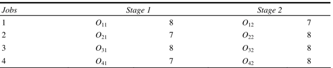
Let consider a HFS of dimension 4 × 2 (i.e. 4 jobs and 2 stages) with the first stage composed of only one machine M1, the second stage of two machines M21 and M22
(Table 1). The allowed depth (d) is fixed at 2. Table 1 Processing times of a 4 × 2 hybrid flow shop
Jobs Stage 1 Stage 2
1 O11 8 O12 7
2 O21 7 O22 8
3 O31 8 O32 8
4 O41 7 O42 8
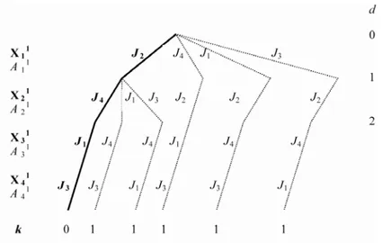
Figure 4 shows the initial solution (0-discrepancy) provided by EST-SPT rule (in the first stage) which gives the following order for the job selection: (J2, J4, J1, J3)
(the lexicographical order is applied for ties breaking). The makespan of the obtained solution is equal to 38. This latter value of makespan is considered as the first upper bound value of the problem: UB = 38.
The neighbourhood associated to 1-discrepancy of this initial solution, as seen in Figure 5, consists of the following sequences (in bold the job upon which is done the discrepancy): d = 1 d = 2 J4, J2, J1, J3 J1, J2, J4, J3 J3,J2, J4, J1 J2, J1, J4, J3 J2, J3, J4, J1
Figure 4 Initial solution
All resource allocation variables take the same value 1 1
i
A =M because we have only one machine at the first stage.
Figure 5 The neighbourhood of the initial solution
For each of these subsequences, the next iteration of our algorithm schedules all the jobs and computes at each node the value of the LB. We use the LBC bound presented in Section 3. We start by the first sequence {J4, J2, J1, J3} and we calculate the LB at each
node. Consider the subset Y = {J4, J2, J1}, one has:
( ) 22 8 (1) ACT Sch ( ) 30; MCT ( ) 22 1 s Y + S Y ⎡ ⎤= = ⎡ ⎤= ⎢ ⎥ ⎢ ⎥ ⎣ ⎦ ⎣ ⎦
Thus, ( ) LBM Sch ( )s 30 8 38 Y ⎡ ⎤ = + = ⎢ ⎥ ⎣ ⎦ and ( ) LBJ Sch ( )s 22 16 38 Y ⎡ ⎤ = + = ⎢ ⎥ ⎣ ⎦ Consequently ( ) LBC Sch ( )s max(38,38) 38 Y ⎡ ⎤ = = ⎢ ⎥ ⎣ ⎦
This value of LB is equal to the initial upper bound. So, we prune this branch (see Figure 6). The same strategy is applied for the second sequence {J1, J2, J4, J3} and
we obtain at the first node LB = 38. So, we stop the exploration of this branch. Figure 6 Neighbourhood’s exploration
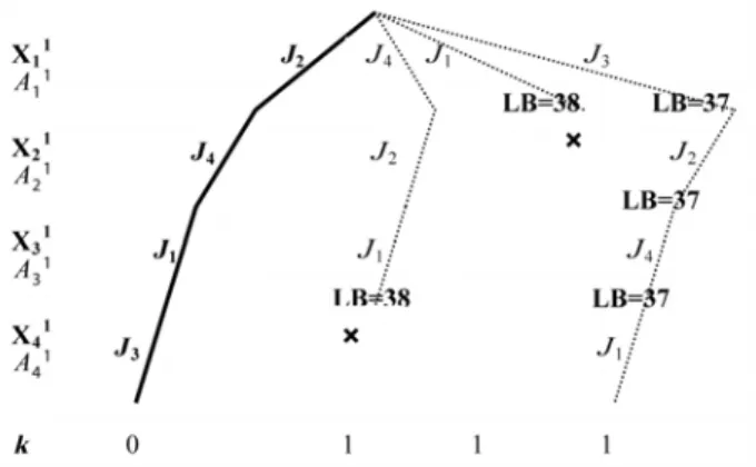
The third sequence{J3, J2, J4, J1} gives a schedule of which the cost is Cmax = 37
(Figure 7). This latter will be considered as the new reference solution and the number of discrepancy is reset to zero. So, we stop the exploration of the neighbourhood of the sequence {J2, J4, J1, J3} and we define a new reference solution’s neighbourhood. This
later is shown in Figure 8. The upper bound is updated and it will be equal to 37 (UB=37).
The neighbourhood associated to 1-discrepancy of the (new) reference solution is composed of the following sequences:
d = 1 d = 2 J2, J3, J4, J1 J4, J3, J2, J1 J1, J3, J2, J4 J3, J4, J2, J1 J3, J1, J2, J4
Figure 8 The neighbourhood of the new reference solution
The calculation of LBs at each node will guide the method for searching in promising branches (see Figure 9). The search will be stopped when there are no more branches to explore. The best solution is given in Figure 7 (Cmax = 37).
Figure 9 Neighbourhood’s exploration for the new reference solution
5 Computational experiments
5.1 Test beds
We compare our adaptation of the DDS method and our proposed CDDS method for solving a set of 77 benchmarks instances which are presented in Carlier and Néron
(2000) and Néron et al. (2001). In Néron et al. (2001), all the problems have been solved using a B&B method operating with use of satisfiability tests and time-bound adjustments. They calculated LBs of the problems and they limited their search within 1800 sec (thus, several instances were not solved to optimality). We also, compare DDS and CDDS methods with AIS strategy (Engin and Döyen, 2004) which is, to the best of our knowledge, the most recent and best solution approach developed so far for solving the HFS.
In our study, we propose to compare our solutions with these LBs. We also run our algorithm within 1800 sec. If no optimal solution was found within 1800 sec, then the search is stopped and the best solution is output as the final schedule. The depth of discrepancy in our methods varies between 3 and 8 from the top of the tree. We have carried out our tests on a Pentium IV 3.20 GHz with 448 Mo RAM. DDS and CDDS algorithms have been programmed using C language and run under Windows XP Professional.
5.2 Results
In Table 2, for all considered problems, we present the best makespan values (BestCmax)
obtained by DDS and CDDS methods among the different value ordering heuristics (SPT, LPT, CJ, SPT-LPT, SPT-CJ, LPT-SPT, LPT-CJ, CJ-SPT, CJ-LPT) and the B&B algorithm of Néron et al. (2001) within 1800 sec. Deviation from LBs is calculated as follows: max Best LowerBound %deviation 100 LowerBound C − = ×
LBs and deviations from such LBs are given in the last four columns.
In Néron et al. (2001), some of the problems are grouped as hard problems. Hard problems consist of the c and d types of 10 × 5 and 15 × 5 problems where for configuration c, machines of the centre are critical and there are two machines in the central stage, while in configuration d there are three machines at all stages. The rest of the problems (all a, b types and 10 × 10 c type problems) are identified as easy problems. In configuration a, the machine of the central stage is critical and there is only one machine at this stage, while in configuration b the first stage is critical with only one machine. As given in Table 2, for a and b type problems better results have been found than for c and d type problems. Indeed, the machine configurations have an important impact on problems complexity that affects solution quality (Engin and Döyen, 2004).
Easy problems instances rapidly converge compared with hard ones. CDDS method takes 5 min in average to obtain all the solutions for easy problems, while DDS method takes 10 min in average. For hard problems, DDS algorithm takes 30 min and CDDS methods takes 25 min in average. Both of B&B and AIS algorithms take 4 min in average when resolving easy problems, while for hard problems B&B algorithm takes 25 min and AIS algorithm takes 10 min. Finally, note that both DDS and CDDS methods have been evaluated in the same computational environment while execution times of B&B and AIS are just reported from Néron et al. (2001) and Engin and Döyen (2004), respectively.
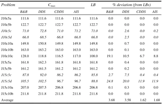
Table 2 Solutions of test problems (italic problems have been identified as hard problems)
Cmax % deviation (from LBs)
Problem B&B DDS CDDS AIS LB B&B DDS CDDS AIS J10c5a 111.6 111.6 111.6 111.6 111.6 0.0 0.0 0.0 0.0 J10c5b 122.7 122.7 122.7 122.7 122.7 0.0 0.0 0.0 0.0 J10c5c 71.0 72.8 71.0 71.2 71.0 0.0 2.6 0.0 0.2 J10c5d 66.8 68.5 66.8 66.8 66.8 0.0 2.5 0.0 0.0 J10c10a 149.8 150.8 149.8 149.8 149.8 0.0 0.7 0.0 0.0 J10c10b 163.0 163.2 163.0 163.0 163.0 0.0 0.1 0.0 0.0 J10c10c 128.0 118.8 116.5 117.0 108.0 19.1 10.5 6.7 8.8 J15c5a 161.8 162.3 161.8 161.8 161.8 0.0 0.4 0.0 0.0 J15c5b 161.2 161.5 161.2 161.2 161.2 0.0 0.2 0.0 0.0 J15c5c 87.8 92.0 86.2 86.2 85.8 2.7 7.5 0.4 0.4 J15c5d 105.5 102.5 96.7 96.7 88.8 24.8 20.0 11.9 11.9 J15c10a 207.0 207.5 206.8 206.8 206.8 0.1 0.3 0.0 0.0 J15c10b 211.8 211.8 211.8 211.8 211.8 0.0 0.0 0.0 0.0 Average 3.68 3.58 1.62 1.68
In Table 3, we compare the efficiency of the four methods for easy and hard problems. As it can be noticed from the table, for easy problems, DDS and CDDS algorithms provide better results than B&B, but for hard problems B&B algorithm and AIS strategy are better than DDS algorithm. Moreover, we observe that CDDS performs remarkably well on both problem classes since it yields better solutions than those provided by B&B and AIS methods.
Table 3 Relative efficiency of the four methods
Method Easy problems Hard problems
% deviation % deviation
B&B 2.21 6.88
AIS 1.01 3.12
DDS 1.42 8.01
CDDS 0.96 3.06
We found that both CDDS and AIS methods give optimal solutions for 61 instances out of 75. Moreover, for the remaining 14 instances, CDDS outperforms AIS for 3 instances, while AIS outperforms CDDS for only one instance.
If all problems are considered, the average deviation from LBs for DDS algorithm is 3.58%, while the average deviation of B&B is 3.68% and for AIS is 1.68%. For CDDS the average is only of 1.63%.
Table 4 presents a comparison between the value ordering heuristics efficiency. For both DDS and CDDS methods, the third rule (CJ) gives always better solutions in a fixed running time.
Table 4 Efficiency of value ordering heuristics
Heuristics SPT LPT CJ SPT-LPT SPT-CJ LPT-SPT LPT-CJ CJ-SPT CJ-LPT
% deviation 4.00 4.93 2.30 2.85 3.23 2.85 3.10 4.00 3.01 Our discrepancy-based methods (DDS and CDDS) prove their contributions in terms of improvement of the initial makespan. Within 1800 sec of CPU time, the deviation of the initial makespan has been reduced with DDS algorithm by nearly 14.7% for hard problems and 9.7% for easy ones. If we consider all problems, the initial makespan has been reduced with DDS algorithm by nearly 10.4%. For CDDS, the initial makespan reduction is about 12%. This percentage is distributed as 20.2% for hard problems and 8.25% for easy ones.
Enhancing CDDS with LBs computation has an important impact. Thus, CDDS method without integration of LBs has been developed and presented in a previous work (Ben Hmida et al., 2006) and its percentage deviation value from LBs was 2.32%.
6 Conclusion and future research
In this paper, two discrepancy-based methods are presented to solve HFS problems with minimisation of makespan. The first one is an adaptation of DDS to suit to the problem under study. The second one, CDDS, combines both CDS and DDS. The two methods are based on instantiation heuristics which guide the exploration process towards some relevant decision points able to reduce the makespan. These methods include several interesting features, such as constraint propagation and LBs computations to prune the search tree, that significantly improve the efficiency of the basic approach. Computational results attest to the efficacy of the proposed approaches. In particular, CDDS outperformed the best existing methods.
Future work needs to be focused on improving the efficiency of the CDDS method. In particular, we expect that the use of the energetic reasoning (Lopez and Esquirol, 1996) would significantly reduce the CPU time. But, this needs to be investigated thoroughly. Moreover, a second research avenue that requires investigation is the implementation of the CDDS method for other complex scheduling problems. In particular, we have already obtained promising results with CDDS for solving the flexible job shop problem.
References
Ben Hmida, A., Huguet, M-J., Lopez, P. and Haouari, M. (2006) ‘Adaptation of discrepancy-based methods for solving hybrid flow shop problems’, Proceedings of IEEE-ICSSSM’06, pp.1120–1125.
Brah, S.A. and Hunsucker, J.L. (1991) ‘Branch and Bound algorithm for the flow shop with multiprocessors’, European Journal of Operational Research, Vol. 51, pp.88–89.
Brah, S.A. and Loo, L.L. (1999) ‘Heuristics for scheduling in a flow shop with multiple processors’, European Journal of Operational Research, Vol. 113, pp.113–122.
Carlier, J. and Néron, E. (2000) ‘An exact method for solving the multiprocessor flowshop’,
Engin, O. and Döyen, A. (2004) ‘A new approach to solve hybrid flow shop scheduling problems by artificial immune system’, Future Generation Computer Systems, Vol. 20, pp.1083–1095. Guinet, A., Solomon, M., Kedia, P.K. and Dussauchoy, A. (1996) ‘A computational study of
heuristics for two-stage flexible flowshops’, International Journal of Production Research, Vol. 34, pp.1399–1415.
Gupta, J.N.D. (1988) ‘Two-stage hybrid flowshop scheduling problem’, Journal of the Operations
Research Society, Vol. 39, pp.359–364.
Gupta, J.N.D. (1992) ‘Hybrid flowshop scheduling problems’, Production and Operational
Management Society Annual Meeting.
Hansen, P. and Mladenovic, N. (2001) ‘Variable neighborhood search: principles and applications’,
European Journal of Operational Research, Vol. 130, pp.449–467.
Haouari, M. and Gharbi, A. (2004) ‘Lower bounds for scheduling on identical parallel machines with heads and tails’, Annals of Operations Research, Vol. 129, pp.187–204.
Haralick, R. and Elliot, G. (1980) ‘Increasing tree search efficiency for constraint satisfaction problems’, Artificial Intelligence, Vol. 14, pp.263–313.
Harvey, W.D. (1995) ‘Nonsystematic backtracking search’, PhD Thesis, CIRL, University of Oregon.
Hoogeveen, J.A., Lenstra, J.K. and Veltman, B. (1996) ‘Preemptive scheduling in a two-stage multiprocessor flowshop is NP-hard’, European Journal of Operational Research, Vol. 89, pp.172–175.
Kis, T. and Pesch, E. (2005) ‘A review of exact solution methods for the non-preemptive multiprocessor flowshop problem’, European Journal of Operational Research, Vol. 164, pp.592–608.
Korf, R.E. (1996) ‘Improved limited discrepancy search’, Proceedings of AAAI-96, pp.286–291. Lee, C.Y. and Vairaktarakis, G.L. (1994) ‘Minimizing makespan in hybrid flow-shop’, Operations
Research Letters, Vol. 16, pp.149–158.
Lin, H.T. and Liao, C.J. (2003) ‘A case study in a two-stage hybrid flow shop with setup time and dedicated machines’, International Journal of Production Economics, Vol. 86, pp.133–143. Linn, R. and Zhang, W. (1999) ‘Hybrid flow shop scheduling: a survey’, Computers and Industrial
Engineering, Vol. 37, pp.57–61.
Lopez, P. and Esquirol, P. (1996) ‘Consistency enforcing in scheduling: a general formulation based on energetic reasoning’, Proceedings of PMS’96, pp.155–158.
Milano, M. and Roli, A. (2002) ‘On the relation between complete and incomplete search: an informal discussion’, Proceedings of CPAIOR’02, pp.237–250.
Moursli, O. and Pochet, Y. (2000) ‘A branch and bound algorithm for the hybrid flow shop’,
International Journal of Production Economics, Vol. 64, pp.113–125.
Néron, E., Baptiste, P. and Gupta, J.N.D. (2001) ‘Solving an hybrid flow shop problem using energetic reasoning and global operations’, Omega, Vol. 29, pp.501–511.
Portmann, M-C., Vignier, A., Dardihac, D. and Dezalay, D. (1992) ‘Branch and bound crossed with G.A. to solve hybrid flow shops’, International Journal of Production Economics, Vol. 43, pp.27–137.
Santos, D.L., Hunsucker, J.L. and Deal, D.E. (1995) ‘Global lower bounds for flow shops with multiple processors’, European Journal of Operational Research, Vol. 80, pp.112–120. Vignier, A. (1997) ‘Contribution à la résolution des problèmes d’ordonnancement de type
monogamme, multimachines (flow shop hybride)’, PhD Thesis, University of Tours, France (in French).