317
Information Management and Business ReviewVol. 6, No. 6, pp. 317-328, December 2014 (ISSN 2220-3796)
Internet Search Volume and Stock Return Volatility: The Case of Turkish Companies
Semen Son Turan MEF University, Istanbul, Turkey
Abstract: This study analyzes the relationship of the volatility ofstock returns and internet search volume (ISV). The dataset consists of 10 Turkish companies listed on the BIST-100 Index of Borsa Istanbul, and encompasses the period between January 2004 - September 2013. The GARCH (1,1) model is applied with two alternative mean specifications. The use of the novel exogenous variable ISV as proxy for investor sentimentis complemented through the inclusion of trading volume.Results show that as the GARCH (1,1) model becomes increasingly nested, volatility persistence declines with however no case of a vanishing G(ARCH) effect.
Keywords: Internet search volume, investor sentiment, stock return volatility, GARCH, Google Trends 1. Introduction
In the 1960s the predominant view in academia was that asset prices in well-functioning markets, with investors holding rational expectations,followed a random walk, and thus cannot be predicted. Built upon this foundation Eugene Fama (1965) put forth the efficient markethypothesis (EMH)stating that it is impossible to beat the market since existing share prices already incorporate and reflect all relevant information.The EMH in its strictest form, states that stock markets are very efficient in swiftly incorporating all information (information on past values, stock fundamentals and private information). Accordingly, even holders of inside information should not be able to make superior returns. Therefore, it should be impossible for investors to beat the market by analyzing past price movements and stock fundamentals since these are already reflected in the prices. Pioneer studies providing empirical evidence for the historical independence of stock prices and showing that fundamental analysis is of no value are those byJensen (1968), Fama, Fisher, Jensen and Roll (1969), and LeRoy (1973). The theoretical framework on the pricing of securities can be traced back to Markowitz (1952, 1959) and the capital asset pricing model (CAPM) where the investor’s aim is to maximize expected return at a given level of risk. A seminal paper by Roll (1977) criticizes tests of the CAPM, demonstrating that any valid CAPM test presupposes complete knowledge of the market portfolio. But, according to the CAPM theory, the market portfolio contains every individual asset in the economy, including human capital, and is, thus, unobservable. Using a stock market index as a proxy for the market portfolio, as commonly used by previous tests, would therefore lead to biased and misleading results.
The direct attack on the EMH premisescomes from Shiller (1981) and LeRoy and Porter (1981), who study equities and bond markets, respectively. Shiller (1981) was the first to attribute his empirical findings of excess volatility to optimistic or pessimistic market psychology. These studies were followed by Schwert (1989), who suggests that volatility of stocks increase during recessions and attributes this movement to operating leverage. What followed was a stream of research encompassing contradictory empirical findings against the general applicability of the EMH (commonly referred to as “market anomalies”). These rest on a series of tests investigating whether publicly available information used in fundamental analysis can be used to improve returns. Many of these papers demonstrate that security prices exhibit volatility clustering, serial correlationand depict that ordinary least squares (OLS) residuals do not display a constant variance as was commonly assumed until then. Consequently researchers started reconsidering the basic premises of Bayesian rationality of investors in evaluating risk and return alternatives and the practical validity of informationally efficient markets. Grossman and Stiglitz (1980) went as far as to argue that the existence of perfectly informationally efficient markets is impossible, since if markets are perfectly efficient, there would be no profit to gathering information.
Along these lines, many researchers argue that patterns of predictability may be traced to irrational traders acting in concert and misinterpreting information. Others, believing in perfect markets, while acknowledging the counter-evidence to non-predictability, argue that any irrational movement would be arbitraged away by rational institutional traders, thus rendering irrational behavior trivial to the stock
318
price formation process. Yet, another strand of literature, posites that there are limits to arbitrage and that prices may deviate to such extremes that even rational traders may no longer be willing,or have the capacity to, make counter-trades. While irrationality is attributed mostly to individuals, there are also studies who accuse institutions of acting upon “noise”. In parallel to empirical findings, finance researchers startedto become aware and acknowledge studies on investor sentiment from behavioral psychology literature. Therein investors trading on noise rather than information were not necessarily consideredirrational. Rather, the concept of bounded-rationality (March and Simon, 1958), exemplifying the limits to human memory and capacity, was embraced. In that regard, non-rational investor behavior was attributed to certain ways of behaving or “heuristics”, the latter denoting “mental shortcuts”- a concept that was introduced by Tversky and Kahneman (1973). Next to various other heuristics, investor sentiment emerged as such heuristic-driven explanation in many finance papers viewing behavioral finance as a sub-discipline.
In its essence, behavioral finance does not attribute decision making processes of investors to simple statistical rules and fundamental market information. It rather stresses the importance of human sentiment. Its roots can be witnessed in the works of Keynes and his concept of “animal spirits (1937) followed by Simon (1955) and March and Simon (1958) who put forth the bounded-rationality principle. These works are succeeded by the theory of cognitive dissonance (Festinger, Riecken and Schachter, 1956), Samuelson’s fallacy of large numbers (1963) and are advanced through the introduction of such concepts as “the availability heuristic”, “representativeness, availability and anchoring and adjustment”, “loss aversion”, “framing”, “under/over-reaction”, “herd behavior”, “overconfidence” by Kahneman and Tversky (1973, 1979), Daniel, Hirshleifer and Subrahmanyam (1998), Shiller (2000) and Shefrin (2000), respectively. Prospect theory (Kahneman and Tversky, 1979) was developed as a more accurate alternative psychological model for decision making under risk, compared to expected utility theory, the latter resting upon the “reality axioms” of von Neuman and Morgenstern (1947). Prospect theory replaces the probabilities put forth by expected utility theory by decision weights which assign value to gains and losses (changes in wealth or welfare) rather than absolute magnitudes. It was Thaler’s work in 1980 that promoted prospect theory to be used as basis for an alternative descriptive theory in economics. Following prospect theory numerous other behavioral heuristics were applied to finance and popularized through several models. One of them is what Barber and Odean (2008) refer to as the “investor sentiment model” in which investors over/underreact to information due to the “overconfidence”. Yet another one is the “noise trader model” by Delong, Shleifer, Summers and Waldmann (1990), (Delong et. al., 1990),which involves investors reacting to irrelevant information.
Overall, the predominant view of rational investors operating in informationally efficient markets marked by no arbitrage opportunities rendering any strategy geared towards the prediction of stock prices valueless, was replaced with the recognition of the limits to arbitrage, investors being rationally-bounded and acting together based on their sentiment. The econometric modelling literature, too, experienced changes over the course of decades. The fluctuation or “variance” of stock price returns over a certain time period, is called stock return volatility or simply “volatility”. Volatility is often times equated with risk and consequently the more stable stock price returns are, the less riskier they are perceived to be. Initial volatility studies in finance and econometrics have come a long way since the 1950s, when Harry Markowitz used standart deviation as a general measure to demonstrate risk reduction through the benefit of diversification. Bollerslev and Wooldridge (1992), refer to risk as “uncertainty” and explain that although the uncertainty of speculative prices was recognized in literature since Mandelbrot (1963) and Fama (1965), it was with the introduction of the Autoregressive Conditional Heteroskedasticity Model (ARCH) of Engle (1982) that researchers started realizing that volatility in high frequency time series data, such as asset returns, is time-varying.
The ground-breaking ARCH Model has changed the landscape of volatility studies and has received numerous extensions. One of the most important ARCH-type models includes the linear Generalized Conditional Heteroskedasticity (GARCH) Model introduced by Bollerslev (1986). Seminal studies on stock price volatility used to consider the residual or the noise term as displaying a constant variance. Thus the OLS regression was used for volatility modelling purposes. However, once empirical findings demonstrating that stock prices contain autocorrelation started populating literature, new models were developed that factored-in autoregressive terms. While believers in informationally efficient markets still exist, there is a growing dominance in literature of believers in the complementary value of behavioral explanations to financial phenomena. Studies presenting investor sentiment as a variable that needs to be analyzed in that realm, have used various direct and indirect measures such as surveys, firm ratios and trading volume
319
among others. However, with the growth of technology and the availability of internet search queries data, these traditional measures are likely to be complemented by a novel proxy: Internet Search Volume. 2. Literature Review
The surge for an understanding of what causes heteroskedasticity present in the error term gave rise to various alternative explanations. One of the most popular of such is the noise trader model by Delong et. al.(1990). The authors borrow the term “noise trader” coined by Kyle (1985) and popularized by Black (1986), to describe investors who trade on pseudosignals and argue that it was them who deterred arbitrageurs to push back prices to their fundamentals thereby creating “noise trader risk”. Investor sentiment models are pioneered by Barberis, Shleifer and Vishny (1998) and Daniel, Hirshleifer and Subrahmanyam (2001). These models commonlyseek to explore the nature of the decision making process of noise traders and use certain sentiment-based heuristics.
Once sentiment was established to contribute to the movements of stock prices, researchers were in need for a quantifiable proxy.One of the most frequently used investor sentiment proxies is trading volume. It is used used mostly in conjunction with the mixture of distributions hypothesis (MDH) developed by Clark (1973), Epps and Epps (1976) and Tauchen and Pitts (1983). According to the MDH, conditional time varying stock return volatility is due to a mixture of distributions, in which the stochastic mixing variable is considered to be the rate of arrival of information flow into the market. According to Fleming, Kirby and Ostdiek (2004), the MDH posits that return volatility is proportional to the rate of information arrival, and hence offers an explanation for the observed heteroskedasticity in returns. Thus, GARCH tests of the MDH imply that if the latent information flowvariable is serially correlated, the trading volumes and return volatilities should also be serially correlated, and there should be a positive relation between them. For testing purposes, trading volume is purported as an exogenous variable in the volatility equation. What follows is that if trading volume can indeed explain volatility persistence then the G(ARCH) parameters should be rendered insignificant and the trading volume parameter magnitudes should be significant and positively related to conditional variance.
Lamoureux and Lastrapes (1990), examining the daily returns of 20 stocks listed on the Chicago Board of Exchange (CBOE), establish that previous GARCH effects tend to mainly disappear upon the inclusion of trading volume. Omran and McKenzie (2000)in their study on Australian stocks, agree with Lamoureux and Lastrapes (1990) that there is a decrease in volatility persistencewith the introduction of trading volume into the variance equation. However, theyargue that,GARCH effects cannot be explained solely based on the serial dependence in trading volume. Many subsequent papers to Lamoureux and Lastrapes (1990), while confirming positive correlations between trading volume and volatility, present less drastic evidence of the disappearance, or a dramatic reduction, of GARCH effects consistent with MDH, through the inclusion of trading volume in stock return volatility equations. The literature on the volume volatility relationship encompasses both, individual stock-level analyses and market-level analyses, the latter reporting much weaker results in the realm of the ideas of Lamoureux and Lastrapes. Thus, it is argued that trading volume presents itself as a relatively better proxy for stock-level analysis (Gursoy, Yuksel and Yuksel, 2008: 200). Baklaci et. al. (2011) argue that investors base their trading decisions on both, information arrivals in the market and beliefs and sentiments about news announcements. The authorsposit that trading volume covers private information and possible noise not fully justified by public news.
While the study of trading volume as an explanatory variable to the volatility of stock returns with the exact extent of its effect still open for discussion, is common in literature, ISV presents itself as a novel proxy of investor sentiment. Apart from seminaleconomic studies (Askitas and Zimmermann, 2009), finance scholars have only very recentlybegun to use ISV data based on names or tickers of stock market indices and individual stocks. Bank, Larch and Peter (2011) using a multivariate panel regression model, investigate the influence of search volume on stocks listed on theGerman Xetra index between January 2004-June 2010. They attribute their findings to uninformed investors and show that an increase in ISV is associated with a rise in trading activity, stock liquidity and temporarily higher future returns. Da, Engelberg and Gao (2011) perform a similar research on all Russell 3000 stocks between 2004-2008. Using a VAR model and panel regressionthey show that ISV is correlated with, but different from, existing proxies of investor attention.Furthermore, they determine that ISV measures attention more timely than do other well-established attention variables.
320
As opposed to the previous two studies which use stock-level data, Dimpfl and Jank (2011) investigate the performance of the DJIA, FTSE100, CAC40, and DAX market indices encompassing the period fromJuly 2006-June 2011 using VAR models and Granger causality analysis. In line with the arguments of Foucault, Sraer and Thesmar (2011), the authors demonstrate that investors' attention to the stock market as measured by Google Trends ISV, rises during periods of high market movements. Furthermore, they argue that a rise in investors' attention, as proxied by name-based keywords, is followed by higher volatility. Another study confirming findings of Da, Engelberg and Gao (2011), using a sample of S&P 500 stocks and their respective ticker-based keywords from Google Insights, is that by Joseph, Wintoki, and Zhang (2011). The authors, through a regression methodology, argue that in the three year period between 2005-2008 ISV, over a weekly horizon, predicts abnormal stock returns and abnormal trading volumes. They conclude that ISV is positively linked to the difficulty of a stock being arbitraged. Vlastakis and Markellos (2012) investigate 30 of the largest stocks traded on the NASDAQ and NYSE and their name-based queries obtained from Google Trends between January 2007-October 2009. The authors analyze the relationship between information supply, as proxied by the Reuters News Scope Archive, and, ISV data from Google Trends, which they consider as proxy for information demand. Employing correlation and causality analyses, they determine that both variables are linked contemporaneously and dynamically. Among other findings, they show that inclusion of both variables results in a significant reduction of volatility persistence (by roughly 58%) using a simple market model mean specification with a GARCH(1,1) model. ISV based on company names is found to be a significant regressor for 13 out 30 stocks with its sign being either a positive or negative.
Bordino et al. (2012) correlate daily ticker-based ISV of NASDAQ-100 stocks obtained from the Yahoo search engine arguing that such represents the attractiveness of trading of a stock. The authors apply time-lagged cross correlation and Granger causality analyses. Results of the correlation analyses indicates that ISV tends to anticipate trading volumes up to a maximum of three days and, establish that, beyond this time frame the correlation between the two variables disappears. Secondly, theyfind a significant lagged cross-correlation relationship between a volatility proxy (the absolute value of price returns) and ISV. As for Granger causality, their findings suggest that query volumes observed today have informative content of tomorrows trading volumes. Latoeiro, Ramos and Veiga (2013), analyze a sample of 36 companies listed on the EURO STOXX 50 Index comprising the largest companies in the Euro area. Their time frame encompasses the period of January 2004-June 2010. To capture abnormal variations of investor attention, the authors construct an abnormal ISV measure from name-based queries comparing current web searches to the average of the previous four weeks. They also construct an abnormal trading volume variable as in Barber and Odean (2008), and, an abnormal returns variable. Conditional volatility measures are obtained using GARCH(1,1) along with a simple market model mean specification. These variables, in addition to a realized volatility variable, form the dependent variables of their study and are sought to be determined through the abnormal ISV variable along with several control and dummy variables through regression analysis. Their results show that an increase in search queries leads to a short-lived increase in volume and volatility, which is rapidly reversed in the following week. The authors attribute the fact that the impact is higher in the following week to the presence of less sophisticated investors.
This study differentiates itself from the above in several aspects:
(1) The time period of this study is the broadest used so far in ISV studies encompassing the period from January 2004-September 2013. Furthermore, to the best of our knowledge, there is no behavioral finance study on an emerging market, nor on the Turkish market per se, using ISV data.
(2) While studies such as Da, Engelberg and Gao (2011), Joseph, Wintoki, and Zhang (2011) and, Bordino et. al. (2012) use ticker-based search queries, Vlastakis and Markellos (2012) and Latoeiro, Ramos and Veiga (2013) use name-based search queries. This study uses name-based ISV data, however, queries are based on Google Trends’Turkish regional searches.
(3) Themeticulous stepwise procedure to arrive at the final sample of analysis, using a combination of eyeball tests and objective criteria, is unique.
(4) Different from previous studies, this study is purely concentrated on the phenomenon of volatility. Aim and Scope: This study aims to analyze the effects of internet search data on stock return volatility, in isolation and together with trading volume, using increasingly nested GARCH(1,1) models. The sample is composed of ten Turkish companies listed on the Borsa Istanbul BIST-100 stock index. Relevant Granger causality testing is applied to determine whether there exists a causal relationship between dependent and independent variables. Lastly, the extent to which the inclusion of the exogenous variables exert influence upon volatility persistence, is examined.
321
Research Questions: The first research question is formulated based on the contraversies surrounding noise trading, trading volume and investor sentiment:
(1) Does investor sentiment, as proxied by ISV, affect stock return volatility?
Grounded in the information flow-trading volume literature, this study explores how these two variables together, exert influence on stock return volatility. Thereby,it concentrates on whether trading volume and /or internet search volume are accountable for volatility clustering and/or G(ARCH) effects. Thus, the second research question becomes:
(2) Do ISV and trading volume have any significant effect on stock return volatility?
Apart from an effect on conditional variance, this study seeks to explore whether there is a temporal causal linkage among stock returns, trading volume and ISV through the third research question:
(3) Is there a causal relationship of stock returns with ISV, and, trading volume and ISV?
As discussed, a bulk of literature, starting with Lamoureux and Lastrapes (1990), posits that inclusion of trading volume in the variance equation leads to decreases in volatility persistence, especially supported for developed markets. To this end, the fourth research question is formulated:
(4) Does the inclusion of ISV and trading volume impact volatility persistence? 3. Data, Sampling and the Model
Data: The BIST-100 index is used as the main index representing the Borsa Istanbul equities market and consists of 100 companies selected among the stocks of firms traded on the national market and the stocks of real estate investment trusts and venture capital investment trusts traded on the collective products market. Stock return and trading volume data is obtained at weekly frequency from Reuters. Stock returns are based on Turkish Lira.
For ISV data collection purposes, Google Trends is used. Google Trends makes available keyword search data as an index that represents search intensity.1 This indexed search volume data is available in a weekly format. Only search queries above a certain volume are being included into the query index. The few previous studies making use of ISV data, are divided between what represents investor sentiment better: the firm name or the ticker symbol.The name-based queries and ticker-based queries of most companies show some significant correlation, however, name-based search queries generate longer and more company-relevant time series. Thus, this study uses name-based search queries. In addition, as opposed to world wide searches, only Turkish regional search queries are used. This is because: (1) there is relatively less-to-none relevant global ISV data available on Turkish companies. For instance,a global Google Trends search for the word “DESA” provides results that belong mainly to the region of Sri Lanka and have nothing to do with Turkish company and (2) using regional Turkey ISV data makes intuitively more sense since foreign-based investors looking to invest into the Turkish market can be considered “sophisticated” and use institutional managers. Moreover it is safe to aasume that, this type of investors would not consult search engines whether to buy particular Turkish stocks.
All data is transformed into logarithmic series and unit root tested using the Augmented Dickey-Fuller test with intercept, with intercept and time trend, and, with neither an intercept nor a time trend. Transformed data, in none of these options, displays unit roots. The descriptive statistics are given in the tables below. Kurtosis and skewness statistics, which are jointly represented by the J-B statistic, show that the price data is not normally distributed. The approximate mean returns for BIST-100 listed companies and (and the BIST-100 Index ) is 0,21% (0,28%). As for standart deviations of the stocks and the BIST-100 Index the values are 5,78% (3,91%). This implies that all stocks, on the average, are more volatile than their respective benchmark index during the period.
1
322
Table 1: Descriptive Statistics for Stock Price ReturnsMean% Medi an% Max% Mi n% SD% SK K J-B p
AKBNK 0,29 0,00 23,15 -21,66 5,85 -0,09 4,47 46,55 0,00 ALARK 0,14 0,00 16,54 -18,30 4,46 -0,33 4,95 88,91 0,00 BANVT 0,21 0,37 47,28 -35,67 6,15 0,71 14,05 2158,52 0,00 DESA -0,04 0,00 27,92 -34,60 6,48 -0,68 7,87 443,57 0,00 KCHOL 0,36 0,00 27,01 -28,14 5,58 -0,20 6,44 207,97 0,00 PETKM 0,20 0,00 22,13 -14,06 4,77 0,39 4,94 76,42 0,00 SANKO 0,00 0,00 21,64 -20,07 4,63 -0,07 6,42 203,85 0,00 THYAO 0,42 0,00 21,87 -27,51 6,00 -0,25 4,64 2,41 0,00 TOASO 0,50 0,75 24,39 -44,83 6,76 -0,82 8,67 606,08 0,00 YATAS 0,01 0,00 24,92 -43,58 7,19 -0,99 10,33 1001,83 0,00 BIST100 0,28 0,59 15,76 -19,27 3,91 -0,45 5,03 103,87 0,00
Note: SD, SK, K, J-B and p stand for standart deviation, skewness, kurtosis, Jarque-Bera statistic and its corresponding p-value, respectively. Prices are based on Turkish Lira.
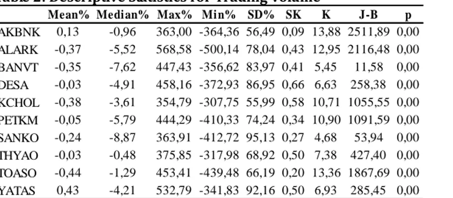
Table 2: Descriptive Statistics for Trading Volume
Mean% Medi an% Max% Mi n% SD% SK K J-B p
AKBNK 0,13 -0,96 363,00 -364,36 56,49 0,09 13,88 2511,89 0,00 ALARK -0,37 -5,52 568,58 -500,14 78,04 0,43 12,95 2116,48 0,00 BANVT -0,35 -7,62 447,43 -356,62 83,97 0,41 5,45 11,58 0,00 DESA -0,03 -4,91 458,16 -372,93 86,95 0,66 6,63 258,38 0,00 KCHOL -0,38 -3,61 354,79 -307,75 55,99 0,58 10,71 1055,55 0,00 PETKM -0,05 -5,79 444,29 -410,33 74,24 0,34 10,90 1091,59 0,00 SANKO -0,24 -8,87 363,91 -412,72 95,13 0,27 4,68 53,94 0,00 THYAO -0,03 -0,48 375,85 -317,98 68,92 0,50 7,38 427,40 0,00 TOASO -0,44 -1,29 453,41 -439,48 66,19 0,20 13,36 1867,69 0,00 YATAS 0,43 -4,21 532,79 -341,83 92,16 0,50 6,93 285,45 0,00
Note: SD, SK, K, J-B and p stand for standart deviation, skewness, kurtosis, Jarque-Bera statistic and its corresponding p-value, respectively.
Trading volume for no company, with J-B p-values being below 5% significance, is close to being normally distributed. Along similar lines, standart deviations for trading volume data is high (75,80%),compared to ISV and stock return series, . This may be an outcome of the fact that companies with different market capitalizations are represented here.
Table 3: Descriptive Statistics for ISV
Mean% Medi an% Max% Mi n% SD% SK K J-B p
AKBNK 0,16 0,00 63,60 -67,25 13,05 -0,08 8,20 574,05 0,00 ALARK -0,37 0,00 99,68 -98,49 25,79 -0,01 4,93 78,83 0,00 BANVIT -0,39 0,00 155,81 -196,61 39,95 -0,35 6,17 182,71 0,00 DESA 0,04 0,00 109,86 -82,10 24,57 0,15 3,95 17,31 0,00 KCHOL -0,41 0,00 138,63 -109,86 30,42 0,09 4,23 26,65 0,00 PETKM -0,17 0,00 156,06 -95,10 31,54 0,74 6,10 205,08 0,00 SANKO -0,10 0,00 96,94 -69,31 23,03 0,37 4,38 42,40 0,00 THYAO 0,06 0,00 97,19 -69,31 18,24 0,24 6,56 273,58 0,00 TOASO -0,44 0,00 87,55 -78,85 31,14 0,06 2,90 0,44 0,00 YATAS -0,21 0,00 74,84 -64,80 17,33 0,29 4,78 60,97 0,00
Note: SD, SK, K, J-B and p stand for standart deviation, skewness, kurtosis, Jarque-Bera statistic and its corresponding p-value, respectively
The average changes in mean ISV values (standart deviations) for BIST-100 companies are 0,18% (25,51%), respectively. These values imply that ISV data is almost four times more volatile than the corresponding stock returns. On a final note regarding descriptives, the three variables, for almost all companies, show serial correlation in the residuals of their respective OLS-regression equations.
323
Each company listed in the BIST-100 Index, has undergone an eyeball test. This is done to eliminate thosewhose names consist of more than one word and/or are generic. Google Trends results are mostly non-existing for unpopular companies, and, if present, may not pertain to them. Since Google Trends data starts in 2004, almost all companies, who had their IPOs later than 2004, are eliminated. The reason for this elimination is to focus on the companies that offer the maximum number of data points in their time series variable. Simultaneously, the news headlines that are featuredon respective ISV index graphs are used to cross-check whether the data actually represents the company under analysis. Lastly, all remaining data is downloaded from Google Trends and checked again to determine whether it is in a format fit for analysis since low-volume data contains many irrelevant “0” values over long time periods. Next comes an interim econometric analysis through data transformation. Log Price Returns and Log ISV are calculated by taking the logarithms of the change in price “Log (Pt/Pt-1)”, ISV data “Log (ISVt/ISVt-1), and trading volume “Log (Vt/Vt-1). This is a common procedure usedin stock return volatility analysis. Consequently, each company is pre-tested for ARCH effects in its residuals. Finally, after application of the GARCH(1,1) model, the resulting parameters need to be checked for their fulfillment of the positivity constraints imposed upon them by the GARCH formulation. A major shortcoming of Turkish firms is that most of them do not have meaningful Google Trends data available, and, among the ones that do, the date interval is not sufficient. Consequently, 10 companies are found to be fit for final analysis purposes.
The Model: There are many proponents of using GARCH models (Bollerslev, 1986) when modelling financial time series data. Among such, is the study by Aybar and Yavan (1998) who examinethe Istanbul Stock Exchange. Comparing various models, the authorsconclude that asymmetry is not a universal phenomenon and suggest symmetric GARCH(1,1) as a better fit. Together the conditional mean and conditional variance equations form a system that is estimated through an iteration process using maximum likelihood. The selection of an appropriate mean specification is thus crucial since the error term derived from that equation is what is being modelled in the variance equation. For the mean specification, previous literature is relied on a set of increasingly nested models is applied. These range from a market model, following Lotaeiro, Ramos and Vega (2013), to an autoregressive AR(1)model, along the lines of Baklaci et. al. (2011), while the latter is more commonly used and theoretically presents itself as a better choice for econometric analysis in behavioral finance. Consistent with Vlastakis and Markellos (2012), this study includes the market return in both mean specifications. After testing for various lags, GARCH(1,1) generates the minimum Akaike Information Criterion “AIC”. The comparative analysis of the adjusted R-squared statistic for both mean specifications shows that the additional autoregressive term does not contribute to an improvement. Thus, only conditional variance equation results for the base market model and increasingly nested versions of such using one exogenous the additional one are being reported. The significance level for all tests is set at 5%. The two mean specifications applied in this study are depicted in equations 1a and 1b, where the former is the market model and the latter is an AR(1) model with the market (BIST-100) return as exogenous variable in the mean:
yt = + x1 +t, where tN(0,
t2 (1a) yt = + x1+yt-1 +t, where tN(0,
t2 (1b)Here, is the constant, is the parameter of the market return x1, is the parameter for yt-1, which is the previous stock returnalso called AR(1), and ?t is a random error with a conditional variance. The difference between the above two mean specifications is that the second model is an AR(1) model specifying that yt, depends linearly on its own previous value. Furthermore, various other mean specifications, where trading volume and ISV variables and their lagged values are included, are tested in the mean equations interchangibly. Since neither ISV nor trading volume have a noteworthy statistically significant impact on the mean, they are exluded from the mean equations. The GARCH(p,q) that is used to model the conditional variance has two characteristic parameters: the number of GARCH terms defined by p referring to the number of autoregressive lags and the number of ARCH terms defined by q referring to the number of moving average lags.
2 1 1 2 1 1 2 t t t
(2)Equation (2) depicts a GARCH(1,1) model where there is a constant (?), an ARCH term () at first lag and a GARCH () term at first lag, with positivity constraints for ?> 0, and parameters ?1 0, ?1> 0, and ?1 + ?1<1.
324
The GARCH(1,1) model solves for the conditional variance as a function of its previous variance, its previous squared return and the long-run variance.The sum of the ARCH and GARCH term parameters is called volatility persistence and refers to how quickly the variance reverts or “decays” toward its long-run average. If persistence is high (low), this means that the decay and the reversion to the mean is slow (quick). If the sum of ARCH (?) and GARCH (?) parameters is 1, this implies there is no mean reversion. If persistence is less than 1, this means there is a reversion to the mean. If persistence is low, this implies a greater reversion to the mean. Table 4 depicts the mean and variance specifications used in this study in an increasingly nested manner.
Table 4: Model Specifications
Model Specification Conditional Mean GARCH -Conditional Variance
1 MM-G(1,1) rt = c + +t 2t= i t-i i ht-i 2 MM-G(1,1)-ISV rt = c + +t 2t = i t-i i t2ici ISVt 3 MM-G(1,1)-ISV-V rt = c + +t 2t = i t-i i t2ici ISVt vi Vt 4 AR(1)M-G(1,1) rt = c + rt -1 + +t 2t= i t-i i ht-i 5 AR(1)M-G(1,1)-ISV rt = c + rt -1 + +t 2t = i t-i i t2ici ISVt
6 AR(1)M-G(1,1)-ISV-V rt = c + rt -1 + +t 2t = i t-i i t2ici ISVt vi Vt Note: (1): rt is expected conditional stock return(2)c is the constant (3) t is residual returns (4) and
are the parameters for market (index) return and previous own value of rt in the mean equation (5) is the constant (or unconditional variance term) (6) i is the parameter for the ARCH term (7)
t-i is news about volatility from the previous period, measured as the lag of the squared residual from the mean equation (the ARCH term) (8) i is the parameter for the GARCH term (9) 2
1
t
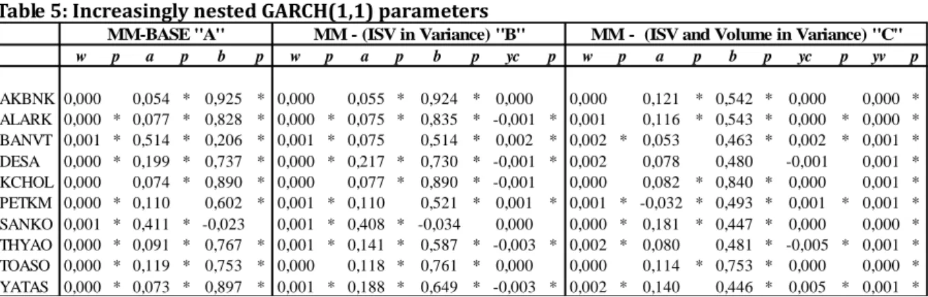
is last period’s forecast variance (the GARCH term) (10) c , v are the parameters for ISV and trading volume, respectively. (11) G stands for GARCH, AR stands for autoregressive at order of 1 and M stands for market (index) returns. The results of pre-testing and post-testing for ARCH effects using Engle’s Lagrange multiplier test (1982), Jarque Bera statistic for normality and Ljung Box Q and Durbin Watson statistics for serial correlation in residuals are analyzed on a company basis.Table 5: Increasingly nested GARCH(1,1) parameters
w p a p b p w p a p b p yc p w p a p b p yc p yv p AKBNK 0,000 0,054 * 0,925 * 0,000 0,055 * 0,924 * 0,000 0,000 0,121 * 0,542 * 0,000 0,000 * ALARK 0,000 * 0,077 * 0,828 * 0,000 * 0,075 * 0,835 * -0,001 * 0,001 0,116 * 0,543 * 0,000 * 0,000 * BANVT 0,001 * 0,514 * 0,206 * 0,001 * 0,075 0,514 * 0,002 * 0,002 * 0,053 0,463 * 0,002 * 0,001 * DESA 0,000 * 0,199 * 0,737 * 0,000 * 0,217 * 0,730 * -0,001 * 0,002 0,078 0,480 -0,001 0,001 * KCHOL 0,000 0,074 * 0,890 * 0,000 0,077 * 0,890 * -0,001 0,000 0,082 * 0,840 * 0,000 0,001 * PETKM 0,000 * 0,110 0,602 * 0,001 * 0,110 0,521 * 0,001 * 0,001 * -0,032 * 0,493 * 0,001 * 0,001 * SANKO 0,001 * 0,411 * -0,023 0,001 * 0,408 * -0,034 0,000 0,000 * 0,181 * 0,447 * 0,000 0,000 * THYAO 0,000 * 0,091 * 0,767 * 0,001 * 0,141 * 0,587 * -0,003 * 0,002 * 0,080 0,481 * -0,005 * 0,001 * TOASO 0,000 * 0,119 * 0,753 * 0,000 0,118 * 0,761 * 0,000 0,000 0,114 * 0,753 * 0,000 0,000 * YATAS 0,000 * 0,073 * 0,897 * 0,001 * 0,188 * 0,649 * -0,003 * 0,002 * 0,140 0,446 * 0,005 * 0,001 *
MM-BASE "A" MM - (ISV in Variance) "B" MM - (ISV and Volume in Variance) "C"
Note: "*", "AR2", denote significance "p" at or below 5%, and adjusted R-squared, respectively. "","","", denote constant, alpha (for ARCH term), and beta (for GARCH term) parameters for the GARCH(1,1) conditional variance equation, respectively. Blank spaces in "p", indicate no significance at or below 5%.“c” denotes ISV parameter. “v” and “VP”denote trading volume parameter and volatility persistence. 4. Empirical Findings
Empirical findings as shown in Table 5, suggest that when ISV is the sole regressor in the conditional variance equation on the average, six out of ten companies have a significant ISV variable. Upon inclusion of the ISV in the conditional variance equation, for one company (BANVT) the significance of the ARCH variable is no longer present. The inclusion of ISV as regressor to the base model does not affect GARCH parameters. However, when trading volume is added as a second regressor, three more companies lose their significant ARCH terms and yet only one company loses its significant GARCH term. With respect to the signs of the coefficients, the results are mixed for the ISV variable, whereas trading volume, for all
325
companies, affects conditional volatility positively. Table 6 shows the parameter values for both mean equation specifications. Both models have similar adjusted R-squared statistics, however, for no company the autoregressive term has any significance.
Table6: Market and AR(1) parameters and Adj R^2 for Base models
p AR2 p AR2 AKBN 1,24 * 0,71 -0,05 0,71 ALARK 0,75 * 0,44 -0,01 0,44 DESA 0,79 * 0,24 -0,05 0,24 PETKM 0,68 * 0,34 -0,02 0,34 SANKO 0,64 * 0,36 -0,07 0,36 THYAO 0,15 * 0,01 -0,02 0,01 TOASO 1,08 * 0,45 -0,09 0,45 YATAS 0,67 * 0,20 0,11 0,22 KCHOL 0,05 0,00 -0,13 0,00 BANVT 0,73 * 0,26 -0,02 0,26 MM AR(1)
Note: and are parameters for market and AR(1) terms, respectively. “*” denotes at or below 5% significance.
When included in isolation to the conditional variance equation, ISV significantly affects almost half of the stocks for both mean specifications, and is negatively-lenient, in terms of sign. Volatility persistence reduces as the model becomes increasingly nested by 7% and 25%, respectively. Trading volume, positively affects the conditional volatility of all stocks, however it does not eradicate the effect of internet search volume for half of the sample. Similarly, trading volume does not account for G(ARCH) effects but there is a slight reduction on the average magnitudes of the G(ARCH) parameters.
Table 7: Volatility Persistence and Change in Volatility persistence
A B C B-A C-B C-A AKBNK 0,98 0,98 0,66 0% -32% -32% ALARK 0,90 0,91 0,66 1% -28% -27% BANVT 0,72 0,59 0,46 -18% -21% -36% DESA 0,00 KCHOL 0,96 0,97 0,84 0% -13% -13% PETKM 0,60 0,52 -13% SANKO 0,63 THYAO 0,86 0,73 0,48 -15% -34% -44% TOASO 0,87 0,88 0,87 1% -1% -1% YATAS 0,97 0,84 0,45 -14% -47% -54% VP Change in VP
Note: MM-BASE "A", MM - (ISV in Variance) "B", MM - (ISV and Volume in Variance) "C" . Blank spaces indicate lack of interpretability due residual serial correlation or failure to comply with non-negativity constraints.
Prior to causality testing, VAR analysis for each company is performed separately. Afterwards, the lag structure is examined and appropriate lag length is chosen according to the minimum AIC value. The AIC is chosen as a criterion for lag order selection as opposed to SIC relying on Ivanov and Lilian (2005) judgments that it produces the most realistic results with small sample sizes.As depicted in Table 8, only SANKO displays a bi-directional temporal ordering of ISV and trading volume at lag 2, while trading volume changes precede ISV changes for YATAS at lag 4.
326
Table 8: Granger CausalityP--> ISV ISV--> P ISV--> V V--> ISV Lag
AKBNK 2 ALARK 1 BANVT 1 DESA 1 KCHOL 1 PETKM 2 SANKO * * 2 THYAO 1 TOASO 5 YATAS * 4
5. Discussion of Findings and Suggestions for Further Research:
This study belongs to a newly emerging group of behavioral finance literature focusing on models that integrate ISV as investor sentiment variable. The implications of the findings of the present study are that (1) there is a relationship between internet search volume and stock return volatility (2) this relationship also holds when trading volume is included as an explanatory variable (3) G(ARCH) effects are not eliminated, meaning that neither internet search volume alone, nor together with trading volume as explanatory variables, do not fully explain the observed heteroskedasticity in stock returns (4) volatility persistence decreases, and thus, mean reversion is quicker with the inclusion of the internet search volume along, an deven more so together with the trading volume variable.
The significance of the present study is that (1) to the best of our knowledge, it is the first study using ISV and a traditional investor sentiment proxy with alternative mean specifications and with data encompassing the broadest time period possible (2) establishes that the AR(1) model and a simple market model are not subordinate to each other in terms of explanatory power (R-squared) (3) it posits that, along the lines of Da, Engelberg and Gao (2011), internet search volume can be used as a proxy for noise trader sentiment of individual investors with respect to the Turkish equity market. (4) it shows that since there is no major apparent temporal ordering found for the majority of stocks, a significant bilateral interaction reflecting, for instance, any return chasing behavior, does not exist. This argument is supported by the findings of Da, Engelberg and Gao (2011), who determine that trading volume is related to internet search volume but explains only a small part of its variation. (5) it is mainly consistent with the findings of Baklaci et al. (2011), who purport a significant and positive influence of trading volume on GARCH effects. The inclusion of the news dummy, as suggested by the authors, as well as an interaction variable of such with trading volume and ISV, might provide further valuable contributions. (6) its findings confirm the literature following Lamoureux and Lastrapes (1990), and, Omran and McKenzie (2000), that inclusion of trading volume decreases volatility persistence of underlying stocks. (7) its findings are not consistent with Lamoureux and Lastrapes (1990), who argue that trading volume, when included in the conditional variance, eradicates G(ARCH) effects. As such, the results of this paper concur with some of the findings mentioned in Omran and McKenzie (2000). (8) it supports the MDH-volume literature in that trading volume and ISV, together and significantly, exert a significant effect upon the conditional variance of the underlying stocks and lower the volatility persistence. It also deems important from a noise trader perspective to emphasize that trading volume data are ex-post outcomes encompassing trades executed by all types of traders, be it individuals or institutions, rational, irrational, or rationally-bounded. ISV data in contrast, is highly likely to represent the individual investor.
As a suggestion for further research thefindings and methodology of the present study can be used as a foundation for further fruitful research in distinct areas. Using the same dataset the methodology can be enriched and findings of other models be compared with the present ones. Most of the time series data, originally of non-stationary character, is subsequently logarithmically transformed to become stationary. Further studies may, for instance, use cointegration tests and thereby avoid losing data points resulting fromthe transformation process. In this study, ISV is obtained through Google Trends, since it has the largest market share of the search engine market. However, ISV data from alternative search engines like Yahoo, Bing and the Russian Search Engine, Yandex, once provided in analyzable format, could be used in combination with the Google-provided ISV index as an aggregate measure. Lastly, various other explanatory variables, besides trading volume, can be added to the model.
327
ReferencesBaklaci, H. F., Tunc, G.., Aydogan, B. & Vardar, G. (2011). The Impact of Firm-Specific Public News on Intraday Market Dynamics: Evidence from the Turkish Stock Market. Emerging Markets Finance and Trade, 47(6), 99-119.
Askitas, N. & Zimmermann, K. (2009). Google econometrics and unemployment forecasting. Applied Economics Quarterly, Duncker & Humblot, Berlin, 55(2), 107-120.
Bank, M., Larch, M. & Peter, G. (2011). Google search volume and its influence on liquidity and returns of German stocks. Financial markets and portfolio management, 25(3), 239-264.
Barber, B. M. & Odean, T. (2008). All that glitters: The effect of attention and news on the buying behavior of individual and institutional investors. Review of Financial Studies, 21(2), 785-818.
Barberis, N., Shleifer, A. & Vishny, R. (1998). A model of investor sentiment. Journal of Financial Economics, 49(3), 307-343.
Bordino, I., Battiston, S., Caldarelli, G., Cristelli, M., Ukkonen, A. & Weber, I. (2012). Web search queries can predict stock market volumes. PloS one, 7(7), e40014.
Bollerslev, T. (1986). Generalized autoregressive conditional heteroskedasticity. Journal of Econometrics, 31(3), 307-327.
Bollerslev, T. & Wooldridge, J. M. (1992). Quasi-maximum likelihood estimation and inference in dynamic models with time-varying covariances. Econometric reviews, 11(2), 143-172.
Black, F. (1986). Noise. The Journal of Finance, 41(3), 529-543.
Clark, P. K. (1973). A subordinated stochastic process model with finite variance for speculative prices. Econometrica, 41, 135–156.
Da, Z., Engelberg, J. & Gao, P. (2011). In search of attention. The Journal of Finance, 66(5), 1461-1499. Daniel, K. D., Hirshleifer, D. & Subrahmanyam, A. (2001). Overconfidence, arbitrage, and equilibrium asset
pricing. The Journal of Finance, 56(3), 921-965.
DeLong, J. B., Shleifer, A., Summers, L. H. & Waldmann, R. J. (1990). Positive feedback investment strategies and destabilizing rational speculation. The Journal of Finance, 45(2), 379-395.
Dimpfl, T. & Jank, S. (2011). Can internet search queries help to predict stock market volatility? (No. 11-15). CFR Working Paper.
Engle, R. F. (1982). Autoregressive conditional heteroscedasticity with estimates of the variance of United Kingdom inflation. Econometrica: Journal of the Econometric Society, 3, 987-1007.
Epps, T. W. & Epps, M. L. (1976). The stochastic dependence of security price changes and transaction volumes: implications for the mixture of distributions hypothesis. Econometrica, 44(2), 305-321 Fama, E. F. (1965). The behavior of stock-market prices. The Journal of Business, 38(1), 34-105.
Fama, E. F., Fisher, L., Jensen, M. C. & Roll, R. (1969). The adjustment of stock prices to new information. International Economic Review, 10(1), 1-21
Festinger, L., Riecken, H. W. & Schachter, S. (1956). When prophecy fails. Minneapolis: University of Minnesota Press.
Fleming, J., Kirby, C. & Ostdiek, B. (2004). Stochastic volatility, trading volume, and the daily flow of information. Rice University, Jones Graduate School Working Paper.
Foucault, T., Sraer, D. & Thesmar, D. J. (2011). Individual investors and volatility. The Journal of Finance, 66(4), 1369-1406.
Grossman, S. J. & Stiglitz, J. E. (1980). On the impossibility of informationally efficient markets. The American Economic Review, 4, 393-408.
Gursoy, G., Yuksel, A. & Yuksel, A. (2008). Trading volume and stock market volatility: evidence from emerging stock markets. Investment Management and Financial Innovations, 5(4), 200-210. Daniel, K., Hirshleifer, D. & Subrahmanyam, A. (1998). Investor psychology and security market under-and
overreactions. The Journal of Finance, 53(6), 1839-1885.
Jensen, M. C. (1968). The performance of mutual funds in the period 1945–1964. The Journal of Finance, 23(2), 389-416.
Joseph, K., Babajide-Wintoki, M. & Zhang, Z. (2011). Forecasting abnormal stock returns and trading volume using investor sentiment: Evidence from online search. International Journal of Forecasting, 27(4), 1116-1127.
Kahneman, D. & Tversky, A. (1973). On the psychology of prediction. Psychological review, 80(4), 237. Kahneman, D. & Tversky, A. (1979). Prospect theory: An analysis of decision under risk. Econometrica:
Journal of the Econometric Society, 3, 263-291.
Keynes, J. M. (1937). The general theory of employment. The Quarterly Journal of Economics, 51(2), 209-223.
328
Kyle, A. S. (1985). Continuous auctions and insider trading. Econometrica: Journal of the Econometric Society, 3, 1315-1335.
Lamoureux, C. G. & Lastrapes, W. D. (1990). Heteroskedasticity in stock return data: Volume versus GARCH effects.TheJournal of Finance, 45, 221–229.
Latoeiro, P., Ramos, S. B. & Veiga, H. (2013). Predictability of stock market activity using Google search queries. Working Paper 13-06. Universidad Carlos III de Madrid.
LeRoy, S. F. (1973). Risk aversion and the martingale property of stock prices.International Economic Review, 5, 436-446.
LeRoy, S. F. & Porter, R. D. (1981). The present-value relation: Tests based on implied variance bounds. Econometrica: Journal of the Econometric Society, 4, 555-574.
Mandelbrot, B. (1963). The variation of certain speculative prices. Journal of Business, 36, 394-419. March, J. G. & Simon, H. A. (1958). Organizations. Wiley.
Markowitz, H. (1952). Portfolio selection*. The Journal of Finance, 7(1), 77-91.
Markowitz, H. (1959). Portfolio selection: Efficient diversificationof investments. Wiley, New York .
Omran, M. F. & McKenzie, E. (2000). Heteroscedasticity in stock returns data revisited: volume versus GARCH effects. Applied Financial Economics, 10(5), 553-560.
Roll, R. (1977). A critique of the asset pricing theory's tests Part I: On past and potential testability of the theory. Journal of Financial Economics, 4(2), 129-176.
Samuelson, P. A. (1963). Risk and uncertainty-a fallacy of large numbers. Scientia, 98(612), 108. Shefrin, H. (2000). Börsenerfolg mit behavioral finance. Schäffer-Pöschel.
Shiller, R. J. (1981). The Use of Volatility Measures in Assessing Market Efficiency. The Journal of Finance, 36(2), 291-304.
Shiller, R. J. (2000). Measuring bubble expectations and investor confidence.The Journal of Psychology and Financial Markets, 1(1), 49-60.
Schwert, G. W. (1989). Why does stock market volatility change over time?The journal of finance, 44(5), 1115-1153.
Simon, H. A. (1955). A behavioral model of rational choice. The Quarterly Journal of Economics, 69(1), 99-118.
Tauchen, G. E. & Pitts, M. (1983). The price variability-volume relationship on speculative markets. Econometrica: Journal of the Econometric Society, 4, 485-505.
Tversky, A. & Kahneman, D. (1973). Availability: A heuristic for judging frequency and probability. Cognitive Psychology, 5(2), 207-232.
Vlastakis, N. & Markellos, R. N. (2012). Information demand and stock market volatility. Journal of Banking & Finance, 36(6), 1808-1821.
Von Neumann, L. & Morgenstern, O. J. (1947). Theory of games and economic behavior. (2nd Ed.) Princeton: Princeton University Press.