Hologram synthesis for photorealistic
reconstruction
Martin Janda,1,*Ivo Hanák,1and Levent Onural2 1
Department of Computer Science and Engineering, University of West Bohemia, Univerzitní 22, Plzenˇ, Czech Republic
2
Department of Electrical and Electronics Engineering, Bilkent University, Ankara TR-06800, Turkey
*Corresponding author: [email protected] Received June 25, 2008; accepted September 21, 2008; posted October 22, 2008 (Doc. ID 97742); published November 24, 2008
Computation of diffraction patterns, and thus holograms, of scenes with photorealistic properties is a highly complicated and demanding process. An algorithm, based primarily on computer graphics methods, for com-puting full-parallax diffraction patterns of complicated surfaces with realistic texture and reflectivity proper-ties is proposed and tested. The algorithm is implemented on single-CPU, multiple-CPU and GPU platforms. An alternative algorithm, which implements reduced occlusion diffraction patterns for much faster but some-what lower quality results, is also developed and tested. The algorithms allow GPU-aided calculations and easy parallelization. Both numerical and optical reconstructions are conducted. The results indicate that the presented algorithms compute diffraction patterns that provide successful photorealistic reconstructions; the computation times are acceptable especially on the GPU implementations. © 2008 Optical Society of America
OCIS codes: 090.1760, 090.1995.
1. INTRODUCTION
Holography is a method to capture the physical nature of light, usually on a planar surface (a hologram), so that when the plate is later illuminated in a proper manner, the originally recorded light is created in a volume [1,2]. If the reconstructed volume filling light is exactly the same as the originally recorded light, an observer will see the original environment, with all of its features includ-ing the three-dimensional (3D) nature of the scene, when looking into the reconstructed light. The fidelity of the re-constructed light is directly related to the 3D reconstruc-tion quality. The major difference between holography and photography is the inability of the latter to record properties of light other than its intensity.
Computation of the hologram pattern due to a given ob-ject is the primary goal of computer-generated hologra-phy, which has a long history [3–6]. Various methods for different situations are reported [3,7–9]. Naturally, there are two major concerns in computer-generated hologra-phy: the quality of the eventual optical reconstruction from these holograms and the speed of computations; the latter is especially important in holographic television ap-plications, where a real-time computation at the frame rate is targeted. Fast computation methods to generate the desired holograms are investigated and reported [10–12], and hardware solutions are employed to increase the speed of computations [13,14].
There are numerous methods that are quite fast for computing holograms of planar objects, including a paral-lel object and image planes as well as slanted planes [15–19]. However, the benefits of holography show them-selves best when the original is a 3D object. Therefore, the fast computation of holograms of not only planar
[two-dimensional (2D)] objects but especially 3D objects is of prime interest.
Digital simulation of optical diffraction and holography invariably starts with discretization of the problem. That necessitates understanding the effects of sampling and quantization. Such effects are much more complicated and interesting for diffraction and holographic patterns than for more common applications, as analyzed in [20–22].
In this paper, we present a complete discrete computa-tional procedure that yields a planar discrete hologram of a given 3D object (or a 3D environment). The object is de-scribed in an abstract manner, as usual in computer graphics, in the form of a 3D geometric structure whose surfaces possess realistic texture and optical reflection properties. Naturally, the problem is similar, in many as-pects, to the classical rendering problem in computer graphics [23–25]; however, the holography case involves coherent light and does not possess classical camera with a lens. The simulation of coherent light requires the in-corporation of the phase into the calculations. Rendering without a classical camera model requires accumulation of light incident from different directions at the points on the hologram plane.
Our computational approach is fundamentally different from the approaches outlined above since it can handle complicated realistic surface structures with occlusions and realistic light reflectivity properties. Furthermore, the proposed discretization scheme allows easier imple-mentations in different computational environments such as graphics processing units (GPUs) or parallel computers in addition to implementations in classical central processing unit- (CPU-) based architectures. Our
macrogeometric-structure model is a classical triangular mesh; however, we are able to accommodate a very large number of triangles to achieve realistic shapes. Further-more, we employ a quite complicated surface reflectivity model to render holograms that then provide realistic 3D image reconstructions. A complete mathematical model adopted for diffraction and subsequent holographic re-cording is presented in Section 2. As commonly utilized in the literature, we also employ the so-called source model in the computations; this is an approximation, much more efficient than the accurate field model, and it provides quite good results for most 3D object shapes [11,26–29]. The discretization of the continuous model is given in Sec-tion 3. We employ a photorealistic surface complexity that consists of dense triangular meshes; furthermore, we im-pose additional restrictions on the surface geometry, as described in Section 4. The details of the algorithm to achieve an efficient computation is presented in Section 5. Implementations on distributed architectures and on GPUs for improved speed are given in Sections 6 and 9, respectively. Fresnel approximation together with its jus-tification is given in Section 7, followed by an associated acceleration method based on a stored and properly zoomed Fresnel kernel given in Section 8.
In addition to numerical reconstructions, we tested our generated holograms also by optical reconstructions using state-of-the-art spatial light modulators (SLMs) [30]. Both numerical and optical results are presented in Sec-tion 10. Finally, conclusions are drawn in SecSec-tion 11.
2. BASIC MODEL FOR HOLOGRAPHIC
SETUP
The basic mathematical formulation that we adopt for dif-fraction and hologram formation due to a 3D object or a scene is presented in this section.
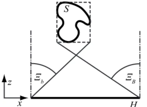
We consider the geometry shown in Fig. 1. Here we have a surface S that radiates light with a directional am-plitude distribution A共s,rˆ兲, where s represents the coor-dinates of a point on S, and rˆ is the unit vector indicating the reverse direction of radiation from s; A共s,rˆ兲 is a complex-valued function. The intensity 兩A共s,rˆ兲兩2 is the
light power emanating from the surface per unit area per
unit solid angle at the point s on S. We have the hologram plane H, where we want to compute the optical field due to the monochromatic coherent illumination from the sur-face S. We chose the hologram plane H as the z = 0 plane. When we consider monochromatic coherent light propagation from the surface S, the field u共x兲 at an arbi-trary point x苸H is modeled as
u共x兲 = c
冕
Sx
A共s,rˆ兲exp共ikr兲
r 共nˆH· rˆ兲dS,
r = s − x, r =兩r兩, rˆ = r/r, 共1兲
where nˆHis the unit normal vector to the hologram plane
H, k = 2/, and is the wavelength. The range of inte-gration Sxrepresents the segments of S that are not oc-cluded when looking from the point x. For convenience, we will drop the complex constant c for the rest of the analysis.
The model adopted above is rather different from con-ventional hologram representations; however, it is more appropriate for our purposes since it associates the holo-gram formation process with computer graphics concepts very conveniently. The directional amplitude distribution A共s,rˆ兲 is directly related to local 2D Fourier transform of the local complex texture (amplitude) on S at s, and therefore, the integral gives a 2D space-frequency repre-sentation for u共x兲. Local frequencies at the location s are directly associated with propagation directions of local plane waves propagating away from s, and the associated complex amplitudes corresponding to those frequencies determine the amplitudes and phase variations of these waves. Therefore, the model violates rigorous mathemati-cal foundations since we need a surface patch, and not a surface point, to describe the local frequency content. We can also state that a point source should have a uniform directional radiation pattern; that violates the nonuni-form possibilities implied by the adopted model. Finally, the amplitude decay by 1 / r is associated with a point source, and other directional radiation patterns as adopted may violate that, as well. A rigorous analysis based on local directional radiation pattern variations, and therefore local frequency content of the surface pat-tern, inevitably brings the associated uncertainity prin-ciple into the model. Such a rigorous analysis is beyond the scope and the purpose of this paper. Instead, in accor-dance with our goal of bringing widely used computer graphics methods to optical field and hologram computa-tion, we adopt a diffraction model as given by Eq. (1), which is an approximation. However, this model is a quite good approximation that can be successfully used to model frequently encountered real-life situations, and thus it is fully adequate for our purposes.
We convert the surface integral above in Eq.(1) via a change of variables to an integration over the solid angle by observing that
dS = r
2d
兩cos兩, cos = nˆs· rˆ, 共2兲 where nˆsis the unit normal to the surface S at the point
Fig. 1. Relation between a differential solid angle dand a dif-ferential surface element dS. The line crossing the surface S de-limits the surface Sxvisible from x and the rest of the surface S.
s. Therefore, the complex valued optical field values u共x兲
over the hologram plane H become
u共x兲 =
冕
⍀ A共s,rˆ兲exp共ikr兲 r 共nˆH· rˆ兲 r2 兩cos兩d, 共3兲 where the integration is over the hemisphere⍀.For convenience, we define a new function A
⬘
共s,rˆ兲 asA⬘共s,rˆ兲 = A共s,rˆ兲 r
2
兩cos兩. 共4兲
In order to evaluate the integral over the solid angle, we further parameterize it in terms of two angles and depicted in Fig.2. Accordingly, the differential solid angle d becomes
d = cos dd, 共5兲
and therefore the optical field over H takes the form
u共x兲 =
冕
−/2 /2冕
−/2 /2 A⬘共s,rˆ兲exp共ikr兲 r 共nˆH· rˆ兲cosdd, 共6兲 where both s and rˆ are functions of共x,,兲. Equation(6) above states the optical field at a point x on H as a super-position of field contributions received from infinitesimal solid angles associated with different directions rˆ by con-sidering the change in phase and amplitude as a conse-quence of the distance between the surface element and the optical field point as well as the attenuation due to ob-liqueness of the incident ray on the hologram plane H from those directions.Note that forming a hologram is straightforward once the optical field on H due to S is found; e.g., a reference beam can be added, and the intensity of the subsequent field is recorded as the hologram [15].
We will discretize the result given by Eq.(6)in the next section to obtain a form that is suitable for digital pro-cessing.
3. DISCRETIZATION
Discretization of Eq.(6)is essential for subsequent digital processing. We start by discretizing the angles and as
l= lD, m= mD, 共7兲
where l and m are integers and D and D are the dis-cretization steps in radians. We also define a regular rect-angular grid of discrete positions xpq on the hologram
plane H as
xpq=共pDx,qDy,0兲 苸 H, 共8兲
where p and q are integers and Dxand Dyare the
discreti-zation steps in meters. Therefore, we label the optical field value at a position xpq as upq. Thus we get the
dis-crete form of Eq.(6)as upq=
兺
l兺
m Apqlm exp关ikrpqlm兴 rpqlm wpqlmcosm, 共9兲where we defined the discrete amplitude variable Apqlm
= A
⬘
共s,rˆ兲DD and the attenuation factor wpqlm= nˆH· rˆ.Note that s and rˆ are functions of共xpq,l,m兲 and
there-fore the amplitude, distance, and attenuation factor are all functions of the indices p, q, l, and m.
We assume that the sampling over the hologram plane H using the sampling intervals Dxand Dydoes not result
in aliasing; this in turn imposes a band-limited u共x兲 with a spatial radian frequency bandwidth of
− Dx ⬍ kx⬍ Dx , − Dy ⬍ ky⬍ Dy , 共10兲
where kxand kyare the frequency variables along the x
and y directions with units in radians per unit length. This bandwidth restriction imposes a limitation on the in-cidence angles of light rays arriving at the hologram plane H from the source surface S, because a plane wave propagating along direction k is a 3D Fourier basis func-tion exp共ik·x兲, whose spatial frequencies along the x, y, and z directions are given by kx, ky, and kz, where
共kx, ky, kz兲=k. For monochromatic light 兩k兩=k=2/,
where is the wavelength of light. Once kx and ky are
fixed for a given wavelength, kz=共k2− kx
2− k
y
2兲1/2 is also
fixed and therefore the direction of propagation is also fixed as k =共kx, ky, kz兲. As a result, for a given Dxand Dy
and the bandwidth as in Eq.(10)to avoid aliasing, we can get the maximum incidence angles as
⌶d= arcsin
冉
kxmax k冊
= arcsin冉
2Dx冊
, ⌿d= arcsin冉
kymax k冊
= arcsin冉
2Dy冊
, 共11兲where kxmax=/Dxand kymax=/Dy[see Eq.(10)]. This
ob-servation further limits the range of l and m indices in Eq. (7) and therefore improves the computational effi-ciency. Note that since the propagation direction of a wave does not change (free-space propagation) as it propagates away (or toward) H, the frequency content, and therefore the bandwidth, will be the same over any hypothetical surface parallel to H. However, in the case of a slanted plane, the same 3D propagation direction will impose other 2D frequency components on the complex field on the plane; the same angle limitations will then impose
Fig. 2. Parameterization of a ray direction rˆ by two anglesand
band-limited patterns with different center frequencies over slanted planes [18]. Therefore, for arbitrary S, the corresponding restriction on the surface texture owing to limitations imposed on the pattern over H can be summa-rized as locally band-limited functions whose local center frequencies are related to the local slope of S. (See Fig.3.) If the slope is zero (parallel to H) the center frequency is zero (low-pass signal), and as the slope increases, the cen-ter frequency also increases. All these statements should be interpreted in the sense of space-frequency represen-tations, in line with the model adopted in the previous section, and therefore the associated uncertainity prin-ciple is in effect.
It is possible to impose further restrictions on the range of l and m in Eq.(7)based on the spatial extent of a finite Sxpq. Considering the bounding box around Sxpq, we see that the range of angles is restricted to 关⌿b,⌿B兴 and
关⌶b,⌶B兴. (See Fig.4.)
Therefore, combining all restrictions above, we fix the range of l and m as
l苸 关Lmin,Lmax兴 :l苸 关− ⌿d,⌿d兴 艚 关⌿b,⌿B兴,
m苸 关Mmin,Mmax兴 :m苸 关− ⌶d,⌶d兴 艚 关⌶b,⌶B兴. 共12兲
4. RESTRICTIONS ON THE SURFACE
GEOMETRY
In this section we will describe the restrictions we choose to impose on the surface geometry S for both analytical and computational convenience.
As we stated in Section 1, our goal is to compute holo-grams for subsequent photorealistic reconstructions. The formulation presented in Section 2 is readily applicable to represent realistic texture reflectance properties since we adopted a space-frequency based description that allows spreading of radiated light within a solid angle. In addi-tion, we target a realistic geometry that would allow the level of detail we expect in a realistic case. To this end, we may choose a triangular mesh that is commonly used in computer graphics, with a large number of triangles. However, as described in Section 3, the adopted aliasing-free sampling strategy imposes restrictions on the complex-valued texture Apqlm over S. Even though it is
possible to satisfy these restrictions, the management of such restrictions will be cumbersome and thus a compu-tational burden. Therefore, we choose to restrict the ge-ometry of S further, in such a way that the management of the complex-valued-texture restrictions becomes easier. To this end, we restrict S to consist only of planar ments that are always parallel to H. However, the seg-ments are discontinuous, since each one may have a dif-ferent distance from H. Such a geometry will ensure that the texture on S will be a slowly varying (low-frequency content) signal as described in Section 3. It is not difficult to implement such restrictions on the texture. However, the discontinuities between the segments could be prob-lematic since they result in phase discontinuities, and that in turn would generate high-frequency components on the texture; this would then violate the restrictions de-scribed in Section 3. Therefore, we restrict the disconti-nuities to be integer multiples of the monochromatic light wavelength . Actually, for convenience, we restrict the distance z from H to a point s on S to be always an integer multiple of. Such a restriction does not create any visual degradation since the introduced step size is 0.4– 0.6m for visible light, whereas the practical dis-tances between the hologram and the object surface is of the order of tens of centimeters in most applications.
The restriction outlined above eases the overall compu-tational burden while conveniently ensuring the condi-tions associated with discretization. However, in order to keep the benefits of working with triangular meshes and still impose the outlined stepwise-discontinuous surface, we adopt a two-step approach. First, we start with a tri-angular mesh S
⬘
to represent S. Then, to get the actual S from S⬘
we quantize the distance from H to be an integer multiple of so that the deviation from the triangular mesh is minimum. (See Fig.5.)5. EFFICIENT COMPUTATION
The basic model for the continuous case and the subse-quent discretization issues, as well as the restrictions on the surface geometry, have already been discussed in pre-vious sections. Therefore, we assume that now the prob-lem is the actual impprob-lementation of the relation given by Eq.(9).
Fig. 3. The propagation angle restrictions associated with aliasing-free sampling of the optical field on H due to Dx(lower cones) determine the propagation angle restrictions associated with the surface S (upper cones). The same restrictions are also in place for the y direction due to Dy.
Fig. 4. Range 关⌶b,⌶B兴 inferred from the bounding box of the
One of the issues during the computation is the accu-racy of the distances rpqlmin Eq.(9)since the distance
af-fects the phase and the hologram computations are sensi-tive to phase errors. The texture on S that is represented by Apqlmin Eq.(9)and the geometry S are input data. We
assume they both comply with the restrictions imposed on them as described in Sections 3 and 4. As a consequence of the already discussed restrictions on the signal u共x兲 and the surface S, it is possible to further restrict Apqlmto
be a real-valued function. This in turn restricts the angu-lar propagation pattern to be symmetric around its cen-ter. (See Fig.3.) Effects of such an additional restriction on the variety of surface textures is not important for our purposes. Computation of other factors in Eq.(9)is rather straightforward. Therefore, we emphasize only the accu-rate computation of the distances, which also includes the accurate computation of the intersection points of rays with S.
Another primary issue is the efficiency of the computa-tions and their suitability for specific implementacomputa-tions, such as an implementation using a commercially avail-able GPU. The actual order of the summations in Eq.(9) and the exploitation of the associated parallelism in com-putation are important in that regard. In this section we describe computational procedures that address both of the issues outlined above.
An important variable of Eq.(9) is the distance to the intersection of a ray and a surface that is nearest to the starting point of the ray on H. This is known as the ray casting method [24,31]. The evaluation of the distance rpqlm between the point xpq on H and the intersection spqlmon S is repeated many times, and therefore it is
com-putationally demanding. We describe an efficient way to find the nearest intersection and then compute the dis-tance rpqlm for the surface S that complies with the
re-strictions imposed on it as described in Section 4. The ray from xpqtoward S is
Rpqlm=兵x : x = xpq+ rrˆlm其. 共13兲
As a consequence, the intersection point spqlm
= Rpqlm艚Sxpqcorresponds to the point of Rpqlmwith a
pa-rameter r = rpqlm.
As we outlined in Section 4, it is convenient to describe the surface S in two steps: first as a triangular mesh S
⬘
and then conversion of mesh structure to a discontinuous surface S whose segments are parallel to H. (See Fig.5.) Therefore, we start with a triangular mesh G =共V,T兲 asour surface S
⬘
, which consists of a set of verticesV and a set of trianglesT. A triangle tABC苸T specifies a triangularsection of a plane between vertices vA, vB, and vC. Normal
of the plane is nABC=共vB− vA兲⫻共vC− vA兲. Our definition of
the mesh G reflects a data structure that is commonly used in computer graphics [25].
In the case of multiple intersections of a ray with the mesh, we need to find the one nearest to xpq. If the set
of intersection points is empty, then we assume that rpqlm=⬁.
As the number of triangles is expected to be high, test-ing each triangle for an intersection might significantly reduce the overall performance. However, we can detect triangles that are completely invisible and omit them. For us a triangle tABCis completely invisible from a point xpq
if 共xpq· nˆABC− vA· nˆABC兲艋0. We denote such triangles as
back facing for xpq.
Furthermore, we observe that in Eq. (9) for l = lc, all
rays Rpqlcmare coplanar with a planeqlc. Considering the
left-handed coordinate system, the planeqlcis
qlc:共qDy− y兲coslc+ z sinlc= 0. 共14兲 This observation leads to efficient evaluation of the inter-section points by adopting a two-step algorithm that is based on slicing the surface. We start by intersecting the mesh G with the plane qlc, and we obtain a slice Wqlc
=共Vqlc,Eqlc兲, where Vqlc is a set of vertices and Eqlc
=兵EAB: EAB苸T艚qlc, vA苸Vqlc, vB苸Vqlc其 is a set of edges.
An edge EABis
EAB=兵x : x = vA+ e共vB− vA兲,e 苸 关0,1兴其, 共15兲
where the vertex vAis the beginning of the edge and the
vertex vBis the end of the edge. Considering only the slice
Wqlcreduces the complexity of intersection search
signifi-cantly. Let us consider the simplest case where lc= 0 and
thereforeq0is parallel with the plane: y = 0. This
spe-cial case is of great significance because each case where l⫽0 can be converted by a geometric transformation to a case where l = 0. The transformation is described later in this section.
Now that we have a set of edgesEq0and a ray Rpq0m,
the goal is to findEq0艚Rpq0m. According to Eqs.(13)and
(15)the ray parameter r and the edge parameter e, corre-sponding to the intersection point are calculated from
xpq+ rrˆ0m= vA+ e共vB− vA兲. 共16兲
When reorganized and assuming rˆ0m=共xr0m, yr0m, zr0m兲,
Eq.(16)becomes a set of two linear equations that can be easily solved for r and e. Since edges are finite line seg-ments, the solution is valid only if e苸关0,1兴. Otherwise the edge is not considered to be intersected.
When searching for the intersections, it is not neces-sary to test all edgesEq0for each m. Since m is ascending,
the anglemis also ascending due to Eq. (7). We use an
easy framework to quickly select for each m only those edges that are intersected by the ray Rpq0m. For each
ver-tex vi苸Vq0and for a fixed q we define an angle Fig. 5. Cross section of a surface S⬘and its decomposition into a
␣ip= arctan
冉
xpq− xvi zvi
冊
, 共17兲
and we sort edges EAB苸Eq0ascendantly by␣Bp. All edges
are oriented so that ␣Ap⬎␣Bp. Then, as long as m
苸关␣Bp,␣Ap兴, the edge EABis intersected by the ray Rpq0m.
Further, letQ=兵EABi 其, Q傺Eq0be a set of active edges,
i.e., edges that are known to intersect with the specific ray Rpq0m. Every time m is increased, edges EAB, ␣Bp
⬍m are added to Q while edges EAB, ␣Ap⬍m are
re-moved fromQ. Since edges EAB苸Eq0are sorted by␣Bpthe
evaluation of the condition␣Bp⬍mis usually performed
only once per edge. We can further improve the algorithm efficiency by employing proper sorting algorithms at dif-ferent stages. Observing that for each edge EAB the
angles ␣Ap and ␣Bp corresponding to samples upq and
up+1qdiffer only a little and therefore the order of edges
do not change much, we use the Bubble Sort algorithm [32] for reordering the edges according to the new values of␣Bp+1since it is known that this algorithm is efficient
for sorting partially sorted data. Nevertheless, for the first sample in a row, the edges are considered irregular and therefore the Quick Sort algorithm [32] is used in this case.
Up to now, we have described the evaluation of a single row for a fixed q and fixed l. The rest of the rows for dif-ferent q are processed in the same fashion. When we move from the row q to the row q − 1, we can exploit the fact that l is kept constant and rows are spaced uniformly. Because of this an efficient triangle scan-line conversion algorithm [33] can be employed to obtain a slice Wq−1,l
from a slice Wql. Thus we complete the computation of all
intersection points for fixed l.
To find all intersection points, we repeat the above pro-cedure for all l苸关Lmin, Lmax兴. Since computing the slice
Wq0 is more convenient than computing arbitrary slice
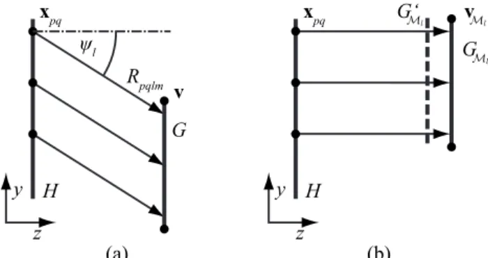
Wql, we proceed with a transformed mesh GMl=Ml兵G其 such that the slice Wql= G艚ql equals the slice Wq0
= GMl艚q0; see Fig.6.
The transformation operator Ml skews the geometry
G =共V,T兲 by modifying vertices v苸V in the direction of the y axis accordingly, i.e. GM
l=共Ml兵V其,T兲. If v苸V then vMl 苸Ml兵V其 is xvM l = xv, yvM l = yv− zvtanl, zvM l = zv 1 cosl . 共18兲
Finally, we modify each intersection point and the cor-responding distance by moving the already computed in-tersection with the triangular mesh S
⬘
to the nearest in-tersection with the stepwise-discontinuous S. We move the intersection along the ray Rpqlm. As a consequence,rpqlmbecomes an integer multiple oflm
⬘
, wherelm⬘ =
nˆH· rˆlm
共19兲 and nˆH=共0,0,1兲 is the normal to the plane H. When rpqlm
is rounded to the nearest integer multiple oflm
⬘
, it isen-sured that the corresponding distance to spqlm on S
⬘
isrounded to the nearest integer multiple of to imply an S as we described in Section 4.
Having the geometry of S, the intersection points of our rays with S together with the associated distances, and the texture Apqlm on S, we are ready to complete the
evaluation of Eq.(9). The algorithm actually follows the steps for the computation of the intersection points we have outlined above: as we evaluate the intersection points and the corresponding distances in the presented order, we immediately compute the associated partial field. First, we compute the partial result upql for all p and
q but for fixed l and then get upqof Eq.(9)as upq=兺lupql .
Not that each upq l
can be interpreted as a “horizontal par-allax only” component of upq[34]. Thus we achieve an
ef-ficient and suitable algorithm, which we call Alg. 1, for evaluating the complete discrete optical field value upq;
naturally, the discrete variables p and q run over a speci-fied finite range. However, there are opportunities for fur-ther acceleration, as presented in the following section.
Algorithm 1. Skeleton of the algorithm for diffraction pattern computation. See the referred sections in the text for
de-tails.
1: for l = Kminto Lmaxdo 䉯 Sec. 3
2: Transform mesh G to mesh GM
l 䉯 Sec. 5
3: for q = −Q to Q do
4: Compute slice Wq0= GMl艚q0 䉯 Sec. 5
5: for p = −P to P do
6: Compute␣Apand␣Bpfor each edge EAB苸Eq0 䉯 Eq.(17)
7: Sort edges inEq0according to corresponding␣Bp
8: LetQ=0
Fig. 6. (a) A mesh G and (b) its modified version GM
l
trans-formed by Eq.(18). The dashed mesh GM
l
⬘ is the skewed mesh G without correction on the distance zv.
9: for m = Mminto Mmaxdo 䉯 Sec. 3 10: Add edge EAB苸Eq0toQ, if␣Bp⬍m
11: Remove edge EAB苸Q from Q, if␣Ap⬍m
12: ifQ⫽0 then
13: Compute all intersection兵rpq0mi 其=R
pq0m艚EAB, EAB苸Q 䉯 Sec. 5
14: Obtain the nearest intersection rpq0m= mini兵rpq0mi 其
15: Add contributionApqlm rpq0m exp
共
i2 rpq0m兲
wpqlmcosmto upq 䉯 Eq.(9) 16: end if 17: end for 18: end for 19: end for 20: end for6. DISTRIBUTED COMPUTING
One strategy to accelerate digital optical field computa-tion is distributing the task on a cluster of computers. A linear speedup is desirable; however, it is practically im-possible to reach such a speedup owing to the sequential parts of the algorithm and the communication necessary to coordinate the computation [35]. In this section we present a distribution scheme that utilizes the algorithm described in the previous section. We aim on minimizing the communication load through an efficient task decom-position.
We assume a homogeneous cluster of nodes connected via a network; i.e., each node is a stand-alone computer with identical configuration. In order to maintain a mini-mal communication load, we exploit the homogeneous cluster environment and we employ a static workload bal-ancing. We algorithmically assign subtasks to nodes prior to the evaluation, and after assigning the subtasks no other communication is necessary until all nodes process their assigned subtasks.
The key feature of the proposed distribution is a decom-position of the algorithm into subtasks. Since we evaluate each sample upq independently of other samples, we can
partition the desired optical field into arbitrary segments, i.e., tiles on H. There are two factors that control the tile selection.
First, the algorithm Alg. 1, which is used for computing the diffraction pattern, exploits preprocessing to speed up the synthesis. It preprocesses the mesh G to speed up the calculation of slices Wq0, and it preprocesses each slice
Wq0to speed up intersection evaluations. In order to limit
the communication load and to avoid synchronization, each node needs to repeat the preprocessing procedure for each subtask. This has a negative effect on the efficiency. In order to minimize the number of repetitions of the pre-processing step for each slice Wq0the tiles are chosen to
be composed of the optical field rows.
Second, the static load balancing requires tasks to fin-ish at the same time to be efficient. Therefore we assign each Nnth row to one tile, where Nn is the number of
nodes. This is based on the assumption that a sequence of Nnslices (Wq0’s) will have a similar number of edges and
vertices. This is justified by the small sampling step Dy,
which is much smaller than the minimal details in com-monly used meshes. Hence, the processing times of all subtasks are similar. To be efficient, the entire subtask has to fit into physical memory of a node. If the subtask
does not fit into node physical memory, we have to use a lower number of rows so that we can generate nsNn
sub-tasks where ns苸N. In the following text, we keep ns= 1 for
the sake of simplicity.
Once the subtasks are established, they are transferred to the corresponding computation nodes for processing. The total number of processed rows in each subtask is equal to the number of rows processed by sequential com-putation. As a consequence, the total time spent on dis-tributed evaluation of the rows is reduced by almost 1 / Nn
compared with the sequential computation.
The distribution described scheme can also be used in conjunction with the GPU-based algorithm by replacing the algorithm used with the one given in Section 9.
7. FRESNEL APPROXIMATION
As already discussed in Section 3 and as summarized by Eq.(12), the propagation angles can be quite small. This is true, in particular, for implementations targeted for op-tical reconstructions using currently available SLMs. Un-der these conditions, the Fresnel approximation is a valid choice, and the term exp共ikrpqlm兲/rpqlm in Eq. (9) is
ap-proximated as [14,36] exp共ikrpqlm兲 rpqlm ⬇ 1 zpqlm exp共ikzpqlm兲 ⫻exp
冋
i k 2zpqlm 共xpqlm 2 + y pqlm 2 兲册
, 共20兲 where共spqlm− xpq兲=共xpqlm, ypqlm, zpqlm兲.The benefits of the Fresnel approximation are even more significant in our case due to restrictions imposed on S as described in Section 4. First of all, since the distance from H to S is always restricted to be an integer multiple of , the phase factor exp共ikzpqlm兲 in Eq. (20) is always
equal to 1. Therefore, we define a generic kernel hz共x,y兲 = 1 z exp
冋
i k 2z共x 2+ y2兲册
, 共21兲where z is a parameter. Observing that
hzpqlm共x,y兲 =2hz共x,y兲, 共22兲
where =共z/zpqlm兲1/2, we can easily compute the needed
ge-neric kernel by properly zooming the kernel and by modi-fying the gain factor. Please note that usually is close to 1, and therefore the associated effect on the amplitude of the kernel is negligible. However, the effect on phase due to scaling of the variables共x,y兲 is important. We exploit this property in the implementation given in Section 8 by computing the generic kernel once and then by zooming it using noninteger interpolation techniques.
8. ACCELERATION BY REDUCED
OCCLUSION
Synthesis of a diffraction pattern, as described in previ-ous sections, is a computationally demanding task. There-fore, it is worthwhile to investigate alternative methods that sacrifice quality somewhat in return for a gain in computational performance. We expect that the loss in quality will be minimal, whereas the gain is significant.
As described in Section 5, our method computes many intermediate horizontal parallax only (HPO) optical fields and then combines those to get the full parallax photore-alistic reconstructions. There is an alternative procedure that needs a fewer number of HPO optical fields and still yields full-parallax but reduced-occlusion reconstructions. The approach is based on computing a full-parallax partial optical field Uqover H formed by a slice Wq0
de-fined in Section 5. However, each slice Wq0is processed
in-dependently of the others without taking into consider-ation the occlusions among the slices. The final diffraction pattern is the sum of the optical fields generated by slices, i.e., U =兺qUq. In other words, the proposed approach
solves the occlusion and solid-surface problems along the x axis, but the occlusions along the y axis are omitted. However, the result is still a full-parallax hologram.
The computational approach shares a part of the algo-rithm presented in Section 5 that calculates the optical field for l = 0. The slicing, point-source generation, and oc-clusion evaluation are the same. The difference in the al-gorithm takes place when a sample upqis processed and
the distance rpqlm to the nearest intersection spqlmis
cal-culated. In the original algorithm, the point source cre-ated at the intersection spqlmcontributes only to a single
sample upq following Eq. (9); that, after all samples are
evaluated, results in an HPO optical field for a slice. How-ever, when we do not care about the occlusions along the y direction, each upq, for a fixed p and variable q, receives a
field contribution from the source at the already com-puted intersection point. We denote the field upqfor fixed
p as the columnpand take advantage of this observation
as described in the next paragraph.
We start by using the result obtained in Section 7 by precomputing and storing a discrete generic kernel. This gives us an optical field on H that would be obtained by a point source located at共0,0,z兲. Using the coordinates of the computed nearest intersection spqlmand the point xpq
atp, we find the appropriate zoom in Eq.(22)and the
spatial shift to be applied to the precomputed optical field. Note that the needed zoom and shift might necessitate subpixel accuracy. We handle this by interpolating the precomputed field linearly along the q direction. Since we compute one column p at a time, only a column of the
precomputed field is scaled and shifted. This results in an efficient calculation. Also, due to the symmetry of the ge-neric kernel, it is sufficient to store only its one quadrant to reduce memory requirements.
9. GPU
The GPU is a central element of a graphics card. It is a specialized processor based on highly parallel architec-tures devoted to speeding up conventional computer graphics tasks such as processing triangular meshes, solving occlusion problems, and rendering final 2D im-ages to be displayed on computer monitors. The current generation of GPUs is programmable, and therefore it is possible to transfer appropriate CPU tasks to the GPU. One such application is digital hologram synthesis [13,14,37,38]. In this section we describe a version of our method that exploits the GPU to decrease computation time.
The GPU is designed to transform triangular meshes and sample them. The sampling task is performed by a hard-wired unit called the rasterizer. The output of the rasterizer is a rectangular grid of the samples to be dis-played on the monitor. We use the GPU to output our op-tical field on H, which is also discretized in a regular rect-angular fashion. To show the relationship between the rasterizer and our approach, let us assume an ortho-graphic projection of the meshes. Then the task of the ras-terizer is equivalent to casting a ray Rpq00 from each
sample point xpq on the grid. The directional vector of
each ray is constant: rˆ00=共0,0,1兲. The rasterizer finds
in-tersections of the rays with the meshes. In further pro-cessing of intersections, the GPU selects the nearest in-tersection by using the depth buffer technique [25]. The diffraction computation described in this paper requires similar computational steps.
In order for the rasterizer to be used to evaluate the in-tersection discussed in Section 5, the vertices of a trian-gular mesh G =共V,T兲 have to be transformed by a trans-formationPlm. The transformationPlmis an extension of
the transformationMlused in Section 5. The extension
into the x axis, however, leads to a hemisphere param-eterization different from Eq.(5). Let us define two angles just for the sake of defining the transformation:¯mand¯l.
The transformation exploits the fact that rˆ00· rˆlm= 1 /lm,
where lm is proportional to the distance rpqlm used in
Eqs.(9)and (13). For the left-handed coordinate system, Plmis Plm=
冤
1 0 0 0 1 0 − tan¯m − tan¯l lm冥
. 共23兲A relation that maps hemisphere parameterization of Eq. (23)to hemisphere parameterization of Eq.(5)is
tan¯m= tanm, tan¯l=
tanl cosm , lm= 1 cosmcosl . 共24兲
After transforming, the z-axis coordinate of the trans-formed vertex v苸Plm兵V其 equals the distance rpqlm. The
whole GPU synthesis is summarized in Alg. 2.
Neverthe-less, there is still the issue of the numerical accuracy of the GPU, which is discussed in the following paragraphs.
Algorithm 2. A skeleton of an algorithm that evaluates the diffraction pattern on the GPU as described in Section 9. For
details on computation, consult the referred portion of the text.
1: for all l = Lminto Lmaxdo 䉯 Sec. 3
2: for all m = Mminto Mmaxdo 䉯 Sec. 3
3: Build transformation metrixPlm 䉯 Eq.(23), Eq.(24)
4: :Let upq⬘ = upq,∀p, q
5: for all Gi債G do
6: Compute fractional part of⌽ilmwith higher precision 䉯 Eq.(25)
7: Render Gito calculate relevant samples upq⬘
8: end for
9: Replace samples upqwith upq⬘
10: end for
11: end for
For performance reasons, the numerical accuracy nowadays of the GPU is limited to 32-bit floating point numbers. This accuracy is insufficient for some parts of Alg. 2. One accuracy problem occurs in Eq.(24)for angles m⬇0 andl⬇0. Regardless of the anglesmandl,lmis
rounded to 1 when stored as a 32-bit floating-point num-ber. This issue is resolved by usinglm− 1 instead oflm. A
more serious accuracy problem occurs during the phase-shift calculation in Eq.(9).
In Eq. (9) the phase of a point source is shifted by pqlm= exp共i2pqlm兲, where pqlm= rpqlm/. The shift
pqlm is stored as pqlm= cos共2pqlm兲+i sin共2pqlm兲.
Since both the sine and the cosine functions are periodic, only a fractional part ofpqlmis needed. For the usual
sce-nario,⬇10−7and r
pqlm⬇10−1, and thus the phase shift
is pqlm⬇106⬃220. This leaves only 4 bits of the
frac-tional part in the mantissa and causes disturbing arti-facts in the reconstruction.
To address the insufficient accuracy we define planes i: z = iDz. The distance ris the length of a ray Rpqlm
be-tween two successive planesiandi+1as depicted in Fig.
7(a). The distance r is finite because 兩l兩⬍/2 and 兩m兩
⬍/2. We choose Dzso that the fractional part of r/ has at least 10 bits. The maximum error of omitted bits is 2⫻2−10⬃10−3Ⰶ1 rad. This also matches the condition
for the validity of the Fresnel approximation [15,36].
In general cases, planesiare used to split the
trian-gular mesh G into many triantrian-gular meshes Gi. As a
con-sequence,pqlm=pqlm
⬘
+⌽ilm, wherepqlm⬘ =lm
zv⬘
, ⌽ilm=lm
iDz
, 共25兲
and zv
⬘
= zv− iDzfor each vertex v苸Gi; see Fig.7(b). If themesh G fits between planesiandi+1, it is not divided.
Since⌽ilmis constant for mesh Giand the given direction rˆlm, it is calculated with higher accuracy outside the GPU
with minimal effect on performance.
10. RESULTS
Results obtained by the various computational proce-dures outlined in previous sections are presented in this section together with comparisons.
Numerical reconstruction results from the computed optical fields are obtained by propagating the fields to planes parallel to H. This is accomplished by taking the discrete Fourier transform (DFT) of the computed optical field, multiplying it by the transfer function correspond-ing to an angular spectrum, and then takcorrespond-ing the inverse DFT [15,19]. We pad the optical field with zeros so that the resolution becomes 8192⫻8192 samples. This
pad-Fig. 7. (a) Evaluation of the longest distance rand (b) decomposition of zvincluding distances proportional to phase shiftspqlm⬘ and
ding reduces the unwanted features associated with the periodicity implied by the DFT. Figures8–13show the in-tensity of the propagated optical fields.
Five different scenes with different levels of complexity and properties are used. The magnitudes of Apqlmover the
object surfaces are obtained according to Phong’s illumi-nation model [39]. The “Photo” is the simplest scene, which is a textured rectangular 2D pattern having a res-olution equal to the resres-olution of the computed optical field. The texture contains small details and smooth in-tensity variations. The second scene, “Primitives”, con-sists of four different simple 3D objects placed along the z axis at different depths. This scene has the longest
dis-tance between the nearest and the farthest object points of all the scenes 共0.2 m兲. The third scene, “Lancaster”, contains a model of the Avro Lancaster airplane. This model consists of over 80,000 triangles, and the magni-tude of the texture is slowly varying. The fourth scene, “Chess,” has several subsurfaces that occlude each other. The last scene, “Bunny”, also has textured sub-surfaces. This scene demonstrates well the ability of our method to handle photorealistic content. The complete parameters of all scenes are provided in Table1.
Figure 8 presents a numerical reconstruction of 2D “Photo” from its optical field computed as described in Section 9. A closeup [Fig.8(b)] is provided together with the original photo [Fig.8(c)] for visual comparison. A loss of detail is visible in the closeup of the reconstruction. The fur of the creature is blurred, but the details of the hairs around its head are still visible. The magnitude of the en-tire computed optical field, which is then used to get the reconstruction, is presented in Fig.8(d).
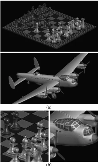
The numerical reconstructions from the optical fields computed by our full-parallax method using “Chess” and “Lancaster” are depicted in Fig.9. Both scenes are
suc-Fig. 8. (a) Numerical reconstruction (intensity) from a GPU-computed optical field. The scene consists of a single textured plane (2D object) parallel to H. The distance between the object plane and the hologram plane is 0.42 m. The resulting image is clipped to 2048⫻1320 pixels. (b) An enlarged detail of the recon-struction is compared with (c) the original texture. (d) The mag-nitude of the entire computed optical field pattern which is then used to get the reconstruction. (The photo is courtesy of Libor Váša).
Fig. 9. (a) Numerical reconstructions (intensity) from optical fields calculated by a GPU and (b) details of the reconstructions. Presented scenes are “Chess” and “Lancaster.” Both reconstruc-tions are computed at a distance of 0.5 m.
cessfully reconstructed. Note that the wood texture present in the scene “Chess” is recognizable in Fig.9(b).
The numerical reconstructions of the scene “Primitives” at different depths are given in Fig.10. The objects at the focused depths are sharp, as expected. Even the farthest object (torus) is successfully reconstructed; see Fig.10(e). Out-of-focus objects yield fringes around them, as ex-pected.
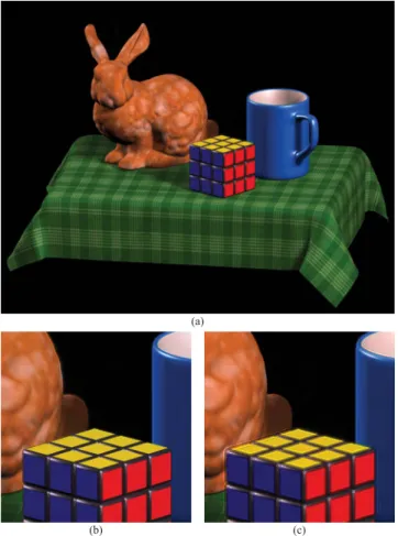
We present the reconstruction of the scene “Bunny” in Fig.11. This reconstruction demonstrates the visual qual-ity that we can achieve with our full-parallax method. Unlike the previous results, the resolution of this optical field is 4096⫻4096 samples. Actually, we computed three different optical fields for three different wavelengths: 650 nm (red), 510 nm (green), and 475 nm (blue). From those three optical fields we reconstructed three separate images and digitally combined them into one color (on-line) image.
In addition to the numerical reconstructions, optical re-constructions were also carried out. Computed optical fields are converted to off-axis holograms by adding a ref-erence beam and then computing the intensity pattern. An SLM that operates in the amplitude-only mode is used for the optical reconstruction. The SLM has a resolution of 1280⫻720 pixels, and the size of each pixel is 12m. The reconstructed optical fields were recorded by a CCD camera stripped of all additional optics. The acquired im-age for the “Lancaster” is shown in Fig.12. The optical re-construction reveals some degradation compared with the numerical reconstruction, but this is expected because of
the much smaller SLM resolution and the noise inherent in the physical setup including the camera.
For a comparison, the numerical reconstructions from optical fields obtained by the full-parallax CPU imple-mentation and the reduced-occlusion impleimple-mentation are shown in Figs.13(a)and13(b), respectively.
We compared the results obtained from the single-CPU, multiple-CPU and GPU implementations of the full-parallax and reduced-occlusion methods. The reconstruc-tions obtained by these methods are almost indistinguish-able visually. The numerical comparison, however, reveals differences that are presented in Table 2. We compared intensity images reconstructed numerically from optical fields computed from the scene “Photo”.
For that purpose we used the maximum difference ⌬max=
maxpq兵兩兩upq兩2−兩upq⬘ 兩2兩其
maxpq兵兩upq兩2其
共26兲 and the mean square error (MSE)
MSE = 1
PQ
兺p兺q共兩upq兩2−兩upq⬘ 兩2兲2
maxpq兵兩upq兩2其
, 共27兲
where upqis a value of the optical field reconstructed from
a result calculated by the CPU full-parallax version (ref-erence optical field); upq
⬘
is the value of the comparedop-tical field; and P and Q are the number of samples along the x and y directions, respectively. From the numbers in Table2it is apparent that the differences for the
distrib-Fig. 10. Numerical reconstructions from a GPU-computed optical field focused at the (a) cone, (b) cylinder, (c) box, (d) sphere, (e) torus. (f) An out-of-focus reconstruction. The optical field is calculated by a GPU. All images are clipped to a resolution of 1100⫻1100 pixels.
uted CPU full-parallax method are negligible. The more pronounced difference measured for the GPU implemen-tation is caused by the reduced numerical accuracy of the GPU and rounding operations of the rasterizer unit. As expected, the reduced-occlusion case gives the highest
dif-ference. This is the result of the different evaluation of the vertical parallax.
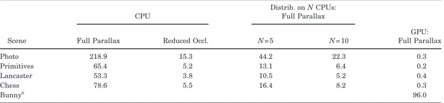
We also measured the processing times associated with the described computational procedures. We tested imple-mentations on a single CPU (Intel Xeon 3.2 GHz, 1 GB RAM), on a cluster of CPU’s (10⫻Intel Xeon 3.2 GHz, 1 GB RAM, 1 Gbps Ethernet), and on a computer equipped with NVidia GeForce 8800 GTX GPU. Taking into account the time requirements of the CPU implemen-tations, we reduced the resolution to 1024⫻1024 samples. The only exception is the scene “Bunny,” which was computed just on a GPU and had a resolution of 4096⫻4096 samples. This resolution demonstrates the ability of the GPU implementation to calculate large op-tical fields in acceptable times. The computation times are summarized in Table3. Considering the rapid devel-opment of the CPU and especially the GPU performance, the measured values should be interpreted only for com-parison purposes. Table 4 lists the speedup factors achieved by different implementations with respect to the single-CPU implementation. It is apparent that the speedup achieved by distributing the computation is ap-proximately linear. What is also apparent is the expected superior computational performance of the GPU
imple-Fig. 11. (Color online) (a) Full-color (online) numerical recon-struction. The color is composed of three components at wave-lengths 650 mn (red), 510 nm (green), and 475 nm (blue). The three optical fields are simultaneously computed by a GPU. (b) A detail of the reconstruction. (c) The same detail reconstructed at a different depth.
Fig. 12. Optical reconstruction from an off-axis hologram. The hologram is obtained from the optical field calculated by a GPU. The incidence angle of the reference beam is 0.758° diagonally to fit the SLM parameters. The reconstruction uses an amplitude-only SLM, and the reconstructed image is captured by a CCD camera without any lens.
Fig. 13. Numerical reconstruction (a) from the CPU computed full-parallax optical field and (b) from the CPU-computed reduced-occlusion optical field. Focus of the numerical recon-struction is approximately at the black pawn in the middle of the picture.
Table 1. Properties of Scenes Used for the Tests
Scene Triangles Projected Sizea (%) Scene Distance (m) Scene Depth (mm) Photo 2 100 0.42 0 Primitives 972 30 0.40 202 Lancaster 83,848 23 0.49 12 Chess 42,566 32 0.49 13 Bunny 84,580 29 0.45 24 a
Percentage of the hologram frame area covered by an orthogonal projection of the scene.
Table 2. Difference Comparisons of the Scene “Photo”
Version ⌬max MSE
Distributed on 5 CPUs 0.003 0.895⫻10−7 CPU reduced occlusion 0.259 0.180⫻10−2
mentation. This is due to the massive parallelism in the GPU architecture. Thus, we expect that by increasing the number of computation nodes of the cluster sufficiently, we can achieve similar results in the distributed environ-ment, as well. Finally, the acceleration by reducing the parallax provides significantly shorter computation time by sacrificing the quality. This approach is therefore quite suitable for a fast preview mode.
11. SUMMARY AND CONCLUSIONS
We have presented detailed computational algorithms for computing optical fields of objects; our primary goal was to achieve photorealistic reconstructions. Therefore, our 3D objects had a large number of triangles in their mesh representations. Furthermore, we adopted realistic sur-face illumination as commonly employed in computer graphics applications. A diffraction model suitable for this goal was adopted and discretization effects were dis-cussed. The model is based on the local angular reflectiv-ity distribution of a textured surface. We developed two algorithms for the full-parallax and reduced-occlusion cases; the former algorithm is implemented on a single CPU, multiple CPU, and a GPU, and the latter algorithm is implemented only on a single CPU.
We conclude that the optical fields obtained from the adopted diffraction model and various implementations of its discrete version provide successful photorealistic re-constructions. The presented algorithms perform well both for simple (planar) objects and quite complicated 3D scenes with large depth. Our conclusions are based both on numerical reconstructions and on optical reconstruc-tions.
In addition to full-parallax implementations, we inves-tigated a reduced-occlusion alternative for faster compu-tation. It is observed that a significant speedup with rather small degradation is possible; this approach is therefore quite suitable for generating fast previews. Op-tical reconstruction quality is lower than numerical re-construction quality. This is due to the SLM resolution used as well as the noise inherent in the physical recon-struction environment.
On the basis of comparisons of different hardware (single-CPU, multiple-CPU, and GPU) implementations, we conclude that all provide almost the same visual qual-ity but that the needed computation times vary signifi-cantly. As expected, GPU implementation is considerably faster.
The proposed solution emphasizes the ability to exploit parallel and distributed computing. We are convinced that the computational complexity of the diffraction-pattern computation cannot be significantly reduced without sacrificing the quality of the reconstructed image. As a consequence of the particular sampling scheme over the object surface, our method allows a straightforward exploitation of acceleration techniques such as computa-tional cluster or GPU. The presented algorithms achieve a speedup factor that is almost a linear function of the number of processors. We showed that holograms with one mega-pixel in size can be computed in tens of minutes using commonly available computational resources.
We conclude that the presented algorithms and their indicated implementations are able to generate holo-grams of arbitrary scenes that have a format common in modern 3D authoring tools used in the multimedia indus-try. This feature is crucial for easy integration into well-established computation pipelines. Furthermore, there
Table 4. Relative Speedup
Scene
CPU
Distrib. on N CPUs: Full Parallax
Full Parallax Reduced Occl. N = 5 N = 10
GPU: Full Parallax Photo 1.00 14.30 4.96 9.81 718.86 Primitives 1.00 12.58 5.00 10.53 327.10 Lancaster 1.00 13.95 5.11 10.16 140.16 Chess 1.00 14.40 4.80 9.58 245.69
Table 3. Computation Times (hr)
Scene
CPU
Distrib. on N CPUs: Full Parallax
Full Parallax Reduced Occl. N = 5 N = 10
GPU: Full Parallax Photo 218.9 15.3 44.2 22.3 0.3 Primitives 65.4 5.2 13.1 6.4 0.2 Lancaster 53.3 3.8 10.5 5.2 0.4 Chess 78.6 5.5 16.4 8.2 0.3 Bunnya 96.0 a
Bunny was used for computing a large共4096⫻4096兲 optical field. The computation time applies for a GPU implementation that simultaneously computes three color chan-nels.
are no drawbacks that would prevent processing of more complicated scenes and computation of larger holograms. Therefore, the presented procedures can be easily used in applications that require larger holograms of larger and more complicated scenes.
ACKNOWLEDGMENTS
This work has been supported by the Ministry of Educa-tion, Youth, and Sports of the Czech Republic under the research program LC-06008 (Center for Computer Graph-ics) and by the Europen Union (EU) project within FP6 under grant 511568 with the acronym 3DTV. The authors thank Metodi Kovachev, Rossitza Ilieva, and Fahri Yaras¸ for the optical reconstructions conducted at Bilkent Uni-versity holographic 3DTV Laboratories. The authors are grateful to Václav Skala for his invaluable comments while this work was conducted.
REFERENCES
1. D. Gabor, “A new microscopic principle,” Nature 161, 777–778 (1948).
2. D. Gabor, “Microscopy by reconstructed wavefronts,” Proc. R. Soc. London, Ser. A 197, 454–487 (1949).
3. L. Onural, A. Gotchev, H. M. Ozaktas, and E. Stoykova, “A survey of signal processing problems and tools in holographic 3DTV,” IEEE Trans. Circuits Syst. Video Technol. 17, 1631–1646 (2007).
4. L. Yaroslavskii and N. Merzlyakov, Methods of Digital Holography, (Consultants Bureau, 1980).
5. G. Tricoles, “Computer generated holograms: an historical review,” Appl. Opt. 26, 4351–4360 (1987).
6. J. Rosen, “Computer-generated holograms of images reconstructed on curved surfaces,” Appl. Opt. 38, 6136–6140 (1999).
7. D. Mendlovic, G. Shabtay, U. Levi, Z. Zalevsky, and E. Marom, “Encoding technique for design of zero-order (on-axis) fraunhofer computer-generated holograms,” Appl. Opt. 36, 8427–8434 (1997).
8. A. G. Kirk and T. J. Hall, “Design of computer generated holograms by simulated annealing: observation of meta-stable states,” J. Mod. Opt. 39, 2531–2539 (1992). 9. V. Arrizón, G. Méndez, and D. Sánchez-de La-Llave,
“Accurate encoding of arbitrary complex fields with amplitude-only liquid crystal spatial light modulators,” Opt. Express 13, 7913–7927 (2005).
10. Y. Sando, M. Itoh, and T. Yatagai, “Full-color computer-generated holograms using 3-D Fourier spectra,” Opt. Express 12, 6246–6251 (2004).
11. K. Matsushima and M. Takai, “Recurrence formulas for fast creation of synthetic three-dimensional holograms,” Appl. Opt. 39, 6587–6594 (2000).
12. M. Cywiak, M. Servin, and F. M. Santoyo, “Wave-front propagation by gaussian superposition,” Opt. Commun. 195, 351–359 (2001).
13. L. Ahrenberg, P. Benzie, M. Magnor, and J. Watson, “Computer generated holography using parallel commodity graphics hardware,” Opt. Express 14, 7636–7641 (2006). 14. A. Ritter, J. Böttger, O. Deussen, M. König, and T.
Strothotte, “Hardware-based rendering of full-parallax synthetic holograms,” Appl. Opt. 38, 1364–1369 (1999). 15. J. Goodman, Introduction to Fourier Optics, 3rd ed.
(Roberts, 2005).
16. G. D. Sherman, “Application of the convolution theorem to Rayleigh’s integral formulas,” J. Opt. Soc. Am. 57, 546–547 (1967).
17. N. Delen and B. Hooker, “Free-space beam propagation between arbitrarily oriented planes based on full diffraction theory: a fast Fourier transform approach,” J. Opt. Soc. Am. A 15, 857–867 (1998).
18. G. Esmer and L. Onural, “Computation of holographic patterns between tilted planes,” Proc. SPIE 6252, 62521K (2006).
19. L. Onural and H. M. Ozaktas, “Signal processing issues in diffraction and holographic 3DTV,” Signal Process. Image Commun. 22, ss169–177 (2007).
20. L. Onural, “Sampling of the diffraction field,” Appl. Opt. 39, 5929–5935 (2000).
21. A. Stern and B. Javidi, “Improved-resolution digital holography using the generalized sampling theorem for locally band-limited fields,” J. Opt. Soc. Am. A 23, 1227–1235 (2006).
22. L. Onural, “Exact analysis of the effects of sampling of the scalar diffraction field,” J. Opt. Soc. Am. A 24, 359–367 (2007).
23. J. T. Kajiya, “The rendering equation,” ACM SIGGRAPH Comput. Graph. 20, 143–150 (1986).
24. A. S. Glassner, Principles of Digital Image Synthesis, (Morgan Kaufmann, 1995), 1st ed..
25. A. Watt, 3D Computer Graphics, 3rd ed. (Addison-Wesley, 2000).
26. M. Lucente, “Optimization of hologram computation for real-time display,” Proc. SPIE 1667, 32–43 (1992). 27. M. Lucente and T. A. Galyean, “Rendering interactive
holographic images,” in Proceedings of SIGGRAPH ’95 (ACM, 1995), pp. 387–394.
28. J. L. Juárez-Pérez, A. Olivares-Pérez, and L. R. Berriel-Valdos, “Nonredundant calculation for creating digital Fresnel holograms,” Appl. Opt. 36, 7437–7443 (1997). 29. G. B. Esmer, L. Onural, H. M. Ozaktas, V. Uzunov, and A.
Gotchev, “Performance assessment of a diffraction field computation method based on source model,” in Proceedings of the 3DTV-Conference 2008 (IEEE Xplore, 2008), pp. 257–260; http://ieeexplore.ieee.org.
30. M. Kovachev, R. Ilieva, P. Benzie, G. B. Esmer, L. Onural, J. Watson, and T. Reyhan, Three-Dimensional Television: Capture, Transmission, and Display, (Springer, 2007), chap. 15.
31. S. D. Roth, “Ray Casting for Modeling Solids,” J. Comput. Graph. Image Process. 18, 109–144 (1982).
32. D. Knuth, The Art of Computer Programming, Volume 3: Sorting and Searching 2nd ed. (Addison-Wesley, 1998). 33. M. Janda, I. Hanák, and V. Skala, “Digital HPO hologram
rendering pipeline,” in Proceedings of EG2006 Short Papers, (Eurographics Association, 2006), pp. 81–84. 34. M. Lucente, “Diffraction-specific fringe computation for
electro-holography,” Ph.D. thesis (MIT, 1994).
35. G. Amdahl, “Validity of the single-processor approach to achieving large scale computing capabilities,” in AFIPS Conference Proceedings, Vol. 30 (American Federation of Information Processing Societies Press, 1967), pp. 483–485. 36. M. Born and E. Wolf, Principles of Optics, 7th ed.
(Cambridge U. Press, 2005).
37. N. Masuda, T. Ito, T. Tanaka, A. Shiraki, and T. Sugie, “Computer generated holography using parallel commodity graphics hardware,” Opt. Express 14, 603–608 (2006). 38. C. Petz and M. Magnor, “Fast hologram synthesis for 3d
geometry models using graphics hardware,” Proc. SPIE 5005, 266–275 (2003).
39. B. Phong, “Illumination for computer generated pictures,” Commun. ACM 18, 311–317 (1975).