Measuring monetary policy for a small open economy: Turkey

(1)

Measuring monetary policy for a small

open economy: Turkey

Hakan Berument

*

Department of Economics, Bilkent University, Ankara 06800, Turkey Received 8 March 2002; accepted 10 February 2006

Available online 13 March 2007

Abstract

This paper proposes a measure to assess the monetary policy for a highly inflationary small open economy: Turkey. The empirical evidence suggests that positive innovations in the spread between the Central Bank’s interbank interest rate and the depreciation rate of the local currency mimic the properties of the tight monetary policy. These innovations, when they are positive, decrease income and prices, and appreciate the local currency. For prices and the exchange rate, the effects are permanent; but for income the effect is transitory.

Keywords: Monetary Policy; Interest rate spreads; Small open economy

1. Introduction

There has been a considerable work on developing monetary models of business cycles. There have also been extensive studies on constructing empirical measures of exogenous monetary policy shocks. Most of these studies perform their analyses for developed coun-tries (seeChristiano et al., 1999and references cited therein). However, central bankers of developing countries, which are also small and open economies, face additional challenges.

*

Tel.: +90 312 290 2342; fax: +90 312 266 5140. E-mail address:berument@bilkent.edu.tr

URL:http://www.bilkent.edu.tr/~berument

(2)

Two of these challenges are related: the problem of currency substitution and central banks’ motive for monitoring their foreign exchange reserves closely. Therefore, the con-struction of a model for developing countries may differ from that of developed countries, and central banks may use their monetary policy tools to accommodate these two policy goals in addition to the ones that the central bankers of developed countries have. First, as regards currency substitution, the public may avoid using domestic currency and prefer using foreign currency to guard itself against inflation. Agents like to hold more of their wealth in foreign currency than in domestic currency if domestic interest rates are lower or if the depreciation of the domestic currency is higher. Second, regarding the level of for-eign exchange reserves, central banks closely monitor these reserves in order to eliminate the risk of speculative attacks or balance of payment crises. Reserves increase as domestic interest rates increase (due to either capital inflows or the decreasing foreign exchange demand of domestic residents) and decrease as the return on foreign exchanges increases. Thus, central banks may use their interest rate and exchange rate policies to achieve their objectives, by moving them in the opposite directions.

This paper uses a new measure to assess monetary policy when interest rates and exchange rates are used simultaneously. In particular, this paper argues that the spread, deﬁned as the extent to which interbank interest rates exceed the depreciation rate of the local currency, can be used as an indicator of the stance of the central bank’s monetary policy for a highly inﬂationary small and open developing country. Using the spread as an indicator of a central bank’s monetary policy does not mean that the bank controls both of these instruments simultaneously, but rather the bank may control one of the two and merely watch the other. However, even in this case, the spread might be used as an indi-cator of monetary policy. This measure is also robust when the central bank switches between pure exchange rate targeting and interest rate targeting regimes. Here, the central bank may cut the liquidity provided to the public by raising interest rates at a given level of depreciation, or it may keep domestic interest rates stable and buy domestic currency from the public by selling foreign currency at a lower rate.

This paper uses Turkish monthly data from 1986:05 to 2000:101to show that tight mon-etary policy is associated with the decrease in income and prices and the appreciation of the local currency, but the effect of monetary policy is not persistent for income. Turkey offers a unique environment for assessing the stance of the monetary policy. Firstly, unlike some other central banks that merely watch markets (e.g., under a currency board), the Central Bank of the Republic of Turkey (CBRT) was actively involved in monetary policy setting during most of the sample period considered, either by influencing interbank inter-est rates or by setting the exchange rate. Secondly, Turkey has been experiencing a high and persistent level of inflation without running into hyperinflation since the mid-1970s. The average annual inflation is 52.3% for the period between 1975 and 2000 and 61.6% for the period that is considered in this study. The high variability of monetary policy changes and the higher level of inflation (or higher level of price level variability) make the relationships between the money aggregates and the macroeconomic variables more visible. Therefore, detecting these relationships will be easier. In other words, the proba-bility of a type 2 error– accepting the null hypothesis when it is false – decreases. Thirdly,

1

The data set is ended in 2000:10 to avoid the beginning of a period that has a series of ﬁnancial crises starting with 22 November 2000 and continuing with 22 February 2001, 7 July 2001 and 11 September 2001, 3 March 2003.

(3)

Turkey has relatively well developed and liberal ﬁnancial markets; in particular, money, foreign exchange and bond markets operate without any heavy regulations that might pre-vent the proper working of the market mechanism for the sample period under consider-ation. Under thin markets, interest rates and exchange rates might move with the initiations of a few speculators (or manipulators). If this were the case, then interest rates and the exchange rates would not be representative of the relative scarcity of domestic and foreign assets. All three of these allow us to assess the eﬀect of monetary policy and the economic outcomes associated with it for Turkey in a reasonable fashion.

Short term interest rates, one of the policy tools of the central bank, cannot be consis-tently below the depreciation rate. If this were the case, the agents would switch their port-folio to hold more in foreign currency than in the domestic currency. Thus, the central bank has an incentive to maintain the interbank interest rate above the depreciation rate; otherwise the domestic money supply would decrease (when agents like to buy foreign exchange from the central bank) at the expense of the central bank’s foreign exchange reserves until the domestic interest rates increase and (or) depreciation rates decrease.2

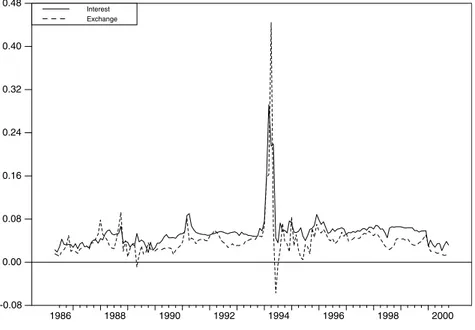
Fig. 1plots the monthly depreciation rate and the interbank interest rate series. Except for a few ﬁnancial crisis periods, interbank interest rates are always above the monthly depreciation rates. Using the interbank rate and the depreciation rate as monetary policy tools and their movements in opposite directions to align the monetary policy is also often perceived by the public as an indicator of monetary policy. This can be observed by news-paper columnists likeGokce (2001) and Yildiz (2002)and even declared publicly by gov-ernments (seeVII. Demirel Government Coalition Protocol, 1991).

2

Under the freely ﬂoating exchange rate regime, the demand for foreign exchange would increase and the demand for local currency would decrease until they came to a state of equilibrium.

1986 1988 1990 1992 1994 1996 1998 2000 -0.08 0.00 0.08 0.16 0.24 0.32 0.40 0.48 Interest Exchange

(4)

By taking the difference between the interbank interest rate and the depreciation rate, we impose the constraint that increasing the interbank rate, which is above the deprecia-tion rate, has an impact on the economy. This imposes the condideprecia-tion that the Central Bank increases the interbank interest rate one-to-one for a given exchange rate depreciation, and the tightness of the monetary policy is determined by how much more the central bank is likely to increase the interbank rate above the depreciation rate. If these two rates are entered separately, it allows the change in the interbank rate to be more or less than the change in the depreciation rate, and this one-to-one relationship that is imposed is used to identify the monetary policy. This scheme has some undesirable properties, as will be discussed later in the text. The next section deals with the specification of the model. Sec-tion3 discusses the effects of the monetary policy and the last section is the conclusion.

2. The speciﬁcation of the model

The identification of the effect of the monetary policy is not a simple task. The reason for this is that actions of the central bank also depend on both the state of the economy and the intention of the central bank for setting up the monetary policy. In order to isolate the effect of a central bank’s policy activities per se, the identification of the components of the central bank’s policy that are not reactive to other variables is crucial. In order to cap-ture this (followingChristiano et al. (1999)and the references cited therein), we specify a vector autoregressive (VAR) model. Here, we measure the monetary policy instrument, which is this spread between the interbank interest rate and the depreciation of the basket, where the basket is the combined TL value of 1 US Dollar plus 1.5 Deutsche Mark.3

The VAR speciﬁcation includes income (y), the logarithm of prices index (p), the log-arithm of the commodity price index in local currency (cp), the loglog-arithm of the exchange rate basket (ex), the spread between the interbank interest rate and the depreciation rate (spread) and the logarithm of money (m). One measure may not capture the level of eco-nomic activity properly. FollowingBernanke and Blinder (1992), we consider an array of variables to measure the economic activity to strengthen our results when the results for each income measures are parallel. However, in Turkey only three of the variables that

Bernanke and Blinder (1992) considered as an economic activity measure are available in monthly frequencies. These three income measures are the logarithm of industrial pro-duction, the private sector capacity utilization rate4and the logarithm of the number of housing permits given by local authorities. The wholesale price index is used for prices. M1 + Repo is also taken as the measure of money. There are two reasons for including Repo in money aggregates: (1) most of the repo transactions were overnight, hence this money aggregate was liquid; (2) agents prefer to repo their savings rather than open deposit accounts since the repo rates are considerably higher. The Repo/Total Demand Deposit rate was 9.54 and the Repo/Total TL Dominated Deposits excluding Repo was 3 _{The choice of foreign currencies and their weights in the basket is declared by the CBRT. This is the basket}

that CBRT follows for its operations.

4 _{Here, the capacity of utilization rate of the private sector is used rather than the total capacity utilization rate}

because the capacity utilization of the government is more likely to be determined by political decisions rather than by the current economic environment. The public considers the capacity utilization rate of the private sector to be more representative of the economic conditions than the total capacity utilization is (see for example,

(5)

0.47 in 2000:10. Hence, the change in interest rates was more likely to affect repo than other components of M1.Sims (1992)notes that central banks may use commodity prices as an indicator of inflation when they set up their reaction. Hence, commodity prices are also included in the VAR specification. All the data except for commodity prices are taken from the data delivery system of the CBRT (http://tcmbf40.tcmb.gov.tr/cbt.html). The commodity price series is taken from the International Monetary Fund – International Financial Statistics tape.

In order to identify the monetary policy shocks, the variables in the VAR are ordered as (yt, pt, cpt, ext, spreadt, mt). This way of ordering is consistent with our basic identifying

assumption that monetary policy setup does not have any contemporaneous eﬀect on income and prices, but income and prices do aﬀect the Central Bank’s policy reaction.

The way that the six macroeconomic variables are ordered may incorporate an extreme information assumption – that policy makers know the current level of income and prices. One way of avoiding this is to use quarterly data. However, the use of quarterly data sug-gests that monetary policy shocks do not affect the income level in the current period, and this may not be true either. Not allowing income and prices to be affected by the current period is more reasonable for monthly data than for quarterly data. It is also reasonable to assume that the Central Bank sets its monetary policy monthly rather than quarterly. Because of the narrow time span for which data are available, we are forced to use monthly data rather than quarterly data. However,Geweke and Runkle (1995), Bernanke and Mihov (1998), Christiano et al. (1996b) and Christiano et al. (1999)indicate that the inference they gather with quarterly data is valid for the inferences gathered with monthly data. Ordering the exchange rate before the spread – implicitly assuming that the exchange rate will affect the spread but not vice versa in the same month – is also consistent with the practice of the CBRT for the sample period we consider, where the CBRT announces the exchange rate every morning before the financial markets open and depreciates the local currency against the basket every day with a constant rate in each month for the period. The public knows the monthly depreciation rate after the first or second business day of each month, but the interest rate is subject to change every day. Therefore, for each month the exchange rate and the daily depreciation rate are constant for the rest of the month. The CBRT tends to change the interbank rate rather than the deprecation rate to align the monetary policy within a given month. Therefore, we can place the exchange rate before spread.

It is important to recognize that the exchange rate enters the VAR specification twice: one as an exchange rate, and the other as the difference between the interbank rate and the percentage change in the exchange rate. This might be considered a problem. Here, we impose the constraint that the difference between the interbank rate and the depreciation rate can be used as an indicator of monetary policy, and we treat the interbank rate above the depreciation rate as a variable separate from the exchange rate. Entering different interest rate spreads along with their components is also common in the literature (for exampleBernanke, 1990, pp. 56–59 andFriedman and Kuttner, 1992, pp. 482–483, Eq. 2 and Table 9), or the difference of a series along with its level can be used (for example

Bernanke, 1983).

The data set used to estimate the model includes observations from 1986:05 to 2000:10. However, when the income measure is taken as the capacity utilization rate, the data set starts from 1991:02 and when the income measure is taken as the number of housing per-mits given by local authorities, the data set starts from 1991:01. The lag length of the VAR

(6)

specification is determined by Hannan–Quinn and Shwarz information criteria, which sug-gest that the lag length should be two. When the regression analysis was performed, each equation had 12 monthly dummies to account for seasonal changes and 3 dummies for the 1994 financial crisis: one for the month when the crisis occurred (April 1994), one for the month before (March 1994), and one for the month after (May 1994). Repo figures are not available before November of 1995; hence, a dummy variable for the period up until 1995:11 is also included. All the variables used here enter the VAR specification in loga-rithmic levels except the spread and the capacity utilization rate, which are entered as rates.

3. The eﬀect of monetary policy shocks

In this section, first the chronological stance of the monetary policy that is suggested by the specification used in this paper will be focused upon. Next, the effect of monetary pol-icy shocks on various aggregates will be analyzed.

3.1. Developments in monetary policy

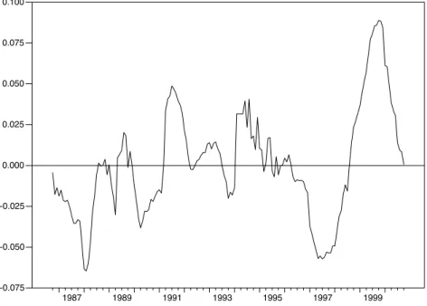
Fig. 2plots the cumulative sum of spread innovation when the industrial production is taken as the income measure. Here, downward movements represent monetary easing, and upward movements represent monetary tightness.Fig. 2suggests that loose monetary pol-icy could be observed during the period from 1986:05 to 1987:12, when Turkey had a series of elections which made it likely that the government would implement loose monetary policies [Sayan and Berument (1997) and Ergun (2000) give the political business cycles

1987 1989 1991 1993 1995 1997 1999 -0.075 -0.050 -0.025 0.000 0.025 0.050 0.075 0.100

(7)

in Turkey]. These elections were local elections for the empty seats in Parliament on Sep-tember 28, 1986; municipality elections on June 8, 1987; the Constitutional Referendum on September 8, 1987; and general elections on November 29, 1987. It is quite likely that the Central Bank adopted loose monetary policy on those days also because it has less inde-pendence from the government (seeBerument and Neyapti, 1999). The second O¨ zal Gov-ernment got the confidence vote from Parliament on December 30, 1987 and this could be the date that indicates the beginning of the tight monetary policy, which was implemented until October 1989, except for the period that precedes the municipal elections on March 26, 1989. In mid-1989, municipal elections were scheduled for June 1990: a loose monetary policy can be seen from the graph. After June 1990, tight monetary policy was imple-mented. Once Prime Minister O¨ zal took the office of the Presidency, Mr. Mesut Yılmaz was elected to be the leader of the Motherland Party and became Prime Minister in June of 1991. He then called for early elections on November 7, 1991 and from the figure loose monetary policy can easily be observed until election day. As a result of the election, Mr. Yılmaz lost and Mr. Demirel formed the new cabinet. Fig. 2also suggests that a tight monetary policy was implemented until April 1993 when the President O¨ zal died and Mr. Demirel took the office of the Presidency. When Ms. Ç iller became the Prime Minister on June 13, 1993, she publicly announced that she would like to decrease interest rates to boost the economy and a loose monetary policy can clearly be observed in the figure until the April 5 financial crisis in 1994.

A stand-by agreement was signed with the IMF in June 1994; however, the agreement was abandoned in September 1995 due to another call for early elections. For the 1996– 1997 period, the CBRT publicly announced that the purpose of the monetary policy was to stabilize the financial markets rather than control increasing inflation. Parallel to that,Fig. 2shows the execution of a loose monetary policy until April 1997. A tight mon-etary policy started to be implemented after Moody’s credit rating institution decreased Turkey’s grade from BA 3 to B 1 for its external debt. Due to the Russian financial crisis which hit in August of 1998, the tight monetary policy continued until the third quarter of 1999. After that, a loose monetary policy was adopted. The CBRT loosened its monetary policy after the Marmara Region Earthquake on August 17, 1999, which cost around 18 000 lives. It is interesting to note that this loose monetary policy continued even with the implementation of the exchange rate based disinflation program in December of 1999. This is what is expected from any exchange rate based disinflation program com-pared to a monetary based disinflation program (see Agenor and Montiel, 1999). To sum up, the identified monetary policy and the developments of political and economic events coincide well.

3.2. Empirical results

In this subsection, a set of empirical evidence on the validity of the speciﬁcation being proposed will be presented.

3.2.1. Spread as a measure of monetary policy

It is necessary to consider whether the estimated impulse responses to monetary policy shocks match the expected movements of macroeconomic variables. Economic theory sug-gests that with monetary contraction, interest rates initially increase and monetary aggre-gates fall. However, following an initial rise, interest rates may decrease due to

(8)

deﬂationary pressure from monetary contraction. Next, with monetary contraction, price levels decline and there is no increase in output level. It is plausible that monetary contrac-tion brings about an output level decrease or a price level increase. However, as long as the monetary policy is exogenous – monetary policy does not systematically respond to eco-nomic factors such as inﬂationary pressure, excess liquidity demand and shocks from the rest of the world – then output level and prices should not increase.

The system that is used here also includes world export commodity prices in domestic currency and the exchange rate. A monetary contraction is not expected to decrease world export commodity prices since Turkey is too small a country to inﬂuence commodity prices. Under a ﬂexible exchange rate, it is expected that currency will appreciate in the short run with the adoption of a tight monetary policy. Moreover, even for a small coun-try, appreciation of the domestic currency may decrease world export commodity prices in terms of domestic currency.

Here, the effect of a tight monetary policy – positive innovation in spread – will be dis-cussed. The first column ofFig. 3shows impulse response functions of industrial produc-tion, prices, commodity prices, exchange rates, spread and money obtained when there is one standard deviation innovation in spread. The middle line shows the point estimates, the other two lines show 5% confidence intervals.5It is important to emphasize some of the observations here. First, the innovation in spread is not persistent. After the third month, the innovation in spread disappears. Second, the effect of monetary policy is tran-sitory on output but persistent in prices.

Tight monetary policy, as measured with positive innovation in spread, has a transitory effect on output. Output levels decrease for the first 5 months even if this is significant in the first two months. The rise in spread is associated with a drop in industrial production following a hump-shaped pattern. This is parallel to the open economy version of the Fuh-rer and Moore model (Fuhrer and Moore, 1995a and Fuhrer and Moore, 1995b) as pre-sented in Walsh (1998, pp. 472–474), and consistent with the evidence on the US (see

Bernanke and Blinder, 1992; Sims, 1992 and Christiano et al., 1996a). The second row of column one suggests that the tight monetary policy permanently decreases the price level.6Tight monetary policy also permanently decreases commodity prices and exchange rates. The evidence on exchange rates is parallel toEichenbaum and Evans (1995), Koray and McMillin (1999) and Kim and Roubini (2000). One standard deviation increase in spread does not persist and ends after the second month. The innovation in spread lasts only for three periods and then cuts oﬀ. This may indicate that the monetary policy of the CBRT is not persistent. However, it may also mean that uncovered interest rate parity holds for a given level of foreign interest rate and the CBRT cannot or does not deviate from it. Lastly, a higher spread decreases money, but this is not statistically signiﬁcant.

Column 2 ofFig. 3repeats the same analysis using the capacity utilization rate of the private sector rather than industrial production. The results are practically parallel but the decreases in price level and exchange rates are not statistically signiﬁcant after the 11th and

5 _{These are computed using the Monte Carlo method with 500 draws from the estimated asymptotic}

distribution of the VAR speciﬁcation as done through the MALCOLM procedure (seeMosconi, 1998) and its covariance matrix as described byDoan (2000).

6

Fig. 3suggests that with the innovation in spread, prices decrease (in a diverging way). We also calculated the impulse responses at longer time spans, in which the decrease in price level stabilizes and is not statistically signiﬁcant after 40 months.

(9)

(10)

10th months, respectively. The last column uses the logarithm of housing permits as a measure of income. There is no qualitative diﬀerence from when the capacity utilization is taken as a measure of income. Importantly, parallel to the overshooting model, when capacity utilization and housing are taken as income measures, domestic currency starts to depreciate after four months of appreciation (seeKoray and McMillin, 1999). The same thing cannot be observed when industrial production is taken as an income measure. Hence, the speciﬁcation used in this paper to identify the monetary policy is on parallel with what the theory suggests.7

3.2.2. Money aggregate as a measure of monetary policy

Traditionally, monetary policy has been identiﬁed with various money aggregates like M0, M1 or M2. Earlier the literature, in particular, followed that pattern (see for example

Barro, 1977 and Mishkin, 1983). In this part, we will try to identify the monetary policy by examining the implied response functions to one standard deviation shock to m as reported in Fig. 4. Column 1 uses industrial production as a measure of income. An increase in money aggregate increases industrial production for 20 months and it is statis-tically significant in the first 9 months. An increase in money supply increases prices and decreases spread. These are parallel to the properties of the expansionary monetary policy and also parallel to the suggestions ofFig. 3. Moreover, there is a decrease in spread as money increases. The effect on the interbank interest rate of an innovation in money aggre-gate might also be of interest. The calculated interbank interest rate (Spread + Deprecia-tion) also suggests that there is a drop in the interbank interest rate for 2 months in a statistically significant fashion (not reported here). On the other hand, importantly, an increase in money decreases both commodity prices and the exchange rate persistently, and that is not what is expected by expansionary monetary policy. Columns 2 and 3 repeat the analysis by using the capacity utilization rate and the logarithm of the number of hous-ing permits as measures of income. The behavior of prices, commodity prices, spread and money are qualitatively similar but exchange rate and income are not.

In order to take the innovations in money aggregate as an indicator of loose money, there are some irregularities: An increase in money (1) decreases the income when housing is used as a measure of income; (2) appreciates the local currency permanently when the income measure is the industrial production and for the ﬁrst four periods when the income measure is the capacity utilization rate; (3) decreases rather than increases the commodity prices for all three income measures. Thus, we may argue that a positive innovation in monetary aggregate does not demonstrate the properties of expansionary monetary policy on exchange rate (when industrial production and the capacity utilization rate are taken as income measures), housing and commodity prices.

3.2.3. Eliminating puzzles

Using the VAR methodology to capture the exogenous part of the monetary policy changes has caused some problems in the literature in the past. The ﬁrst problem is that the empirical evidence might suggest that innovation in monetary aggregates is associated

7

We consider various lag orders for robustness in our results. As the lag order above 6 is considered, even if it is not statistically significant, positive innovation in spread is associated with higher rather than lower prices. This may mean that the results presented in this paper are not robust against alternative specifications. Alternately, it may mean that because of the narrow time span, the high lag order over-specified the model.

(11)

(12)

with rising (rather than decreasing) interest rates – liquidity puzzle (Leeper and Gordon, 1992).Strongin (1995), Christiano et al. (1996a)and others suggested the use of narrow money aggregates like non-borrowed reserves to solve the liquidity puzzle.Sims (1986), on the other hand, suggested separating the money demand and supply shocks by using an identiﬁed VAR model to address the liquidity puzzle.

The second problem is that once the interest rate measure is integrated into the speci-ﬁcation, monetary aggregates no longer cause output in Granger’s sense (Sims, 1980; Lit-terman and Weiss, 1985). This encouragedBernanke and Blinder (1992) and Sims (1992)

to use the innovation in short-term interest rate as a measure of monetary policy change. However, this created additional challenges. When a tight monetary policy is identified with positive interest rate innovations, it seems that prices increase rather than decrease – price puzzle (Leeper and Gordon, 1992; Sims, 1992). Among others,Sims (1992), Sims and Zha (1996) and Christiano et al. (1996a) suggest including commodity prices to account for this puzzle.Kim and Roubini (2000)suggest using a structural identification scheme. The third puzzle suggests that positive innovation in interest rates is associated with the impact of the depreciation of the local currency rather than its appreciation – exchange rate puzzle (Sims, 1992; and Grilli and Roubini, 1995). In our specification, we do not have any of these puzzles.8As a last puzzle, if the uncovered interest rate parity holds, then an increase in the domestic interest rate should lead to persistent depreciation rather than appreciation – forward discount biased puzzle (Eichenbaum and Evans, 1995; and Kim and Roubini, 2000). In this study, we eliminate the last puzzle when the income measure is the capacity utilization rate and housing. However, when the income measure is industrial production, the exchange rate stabilizes after the initial shock. Therefore, the elimination of these puzzles further supports the validity of the specification in this paper. 3.2.4. Other money aggregates

Here M1 plus Repo is used as a money aggregate. It might be necessary to use broader money aggregates; hence, M2 plus Repo (M2R) is also used as a money aggregate.9Fig. 5

reports the impulse responses when one standard deviation shock is given to spread and M2R and when industrial production is taken as a measure of income. An increase in spread decreases income temporarily but decreases prices and exchange rate permanently. However, the increase in spread initially increases the M2R but decreases it later. Even if the initial increase is confusing, this increase is not statistically signiﬁcant.10An increase in M2R decreases prices rather than increasing them. This also supports the proposition that it is not the money aggregate, but the spread that captures the properties of monetary pol-icy. Last, we repeated the exercise for the other two income measures (they are not reported to save space). The results are mostly parallel except that an increase in M2R is associated with higher, not lower, prices.

8 _{These puzzles are addressed in later studies; see}_{Kim and Roubini (2000), Christiano et al. (1999)}_{and the}

references cited therein.

9 _{Hannan–Quinn and Shwarz information criteria suggest that the lag length of the VAR process should be one.}

Therefore, the selected lag length is one when the M2R variable is used as a liquidity measure.

10

It is often argued that tight monetary policy increases firms’ profits by increasing the firms’ non-optional activities (see, for exampleISO (2002)). Firms tend to postpone their investments and increase their bank deposits in order to increase their interest earnings. Thus, tight monetary policy increases bank deposits and M2.

(13)

(14)

3.2.5. Interest rate as a monetary policy tool

In this paper, we argue that the interbank rate innovations, which are above the depre-ciation rate, measure the stance of the monetary policy. To be specific, a positive innova-tion in the depreciainnova-tion rate increases the interest rate innovainnova-tion one-to-one to keep the monetary policy neutral. An increase in the unanticipated part of the interbank rate beyond this one-to-one increase suggests the tightness of the monetary policy. However, including the interbank rate and the depreciation rate separately – rather than using a spread rate – does not impose this constraint to identifying the monetary policy. We allow that the innovation in the interbank rate might be more or less than one to keep the neu-trality of monetary policy. In order to account for this, we entered the depreciation and the interest rate as separate variables in the VAR setting. Specifically, we estimated the 6 var-iable VAR specification that includes y, p, cp, ex, interbank rate and M1R. The first col-umn ofFig. 6reports the impulse response functions when one standard deviation shock is given to interbank rate and when the income measure is industrial production. A positive shock to interbank rate decreases income initially but later increases it; however, they are not statistically significant. It is worth noting that a positive shock to interbank rate increases prices permanently; i.e. the price puzzle is present. Moreover, an increase in the interbank rate depreciates the local currency permanently; i.e. the exchange rate puzzle is present. This suggests that spread is a better indicator of the monetary policy compared to interbank interest rate within the framework we consider here. The second column of

Fig. 6suggests that an increase in money appreciates rather that depreciates the local cur-rency: this is also a puzzle. We repeated the exercise for the other two income measures. (These results and the results of the other impulse response functions are not reported here but are available from the author upon request.) Although, the results were mostly similar for the other two income measures, the exchange rate puzzle disappeared, while the price puzzle remained.

3.2.6. Post-crisis periods

It is often argued that the self-inflicted 1994 financial crisis in Turkey altered the work-ing of the financial markets (seeOzatay, 2000; Alper and Onis, 2003; Ertugrul and Selcuk, 2002). Therefore, we performed the analysis for the post-crisis era by considering the per-iod from 1994:08 to 2000:10. With the positive innovation of the spread, income, prices, commodity prices, exchange rates and money decrease for all the three income measures that we consider in this paper. Thus, the results that we gather from the benchmark spec-ification are robust. On the other hand, a positive innovation in money decreases capacity utilization and housing, and initially (in a statistically significant fashion) appreciates the local currency when the income measure is industrial production.

3.2.7. Impulses with re-ordered variables

Christiano et al. (1996b)discusses the importance of the ordering of the variables in the VAR setting. If income and prices precede the spread, then this type of ordering imposes the extreme information assumption. The CBRT observes these variables in the current time period before it sets the spread. The spread is also used as the first variable when the monetary policy of the CBRT affects all those variables in the current period. The evi-dence gathered with the re-ordered VAR does not conflict with the benchmark specification.

(15)

(16)

3.2.8. Evidence from forecast error variance decomposition

The impulse response functions assess the dynamic eﬀects of monetary policy shocks. Forecast error variance decomposition analysis assesses how monetary policy shocks con-tribute to the volatility of various economic aggregates. There are two reasons for the importance of the latter. First, it helps to assess whether monetary policy shocks have been an important independent source of impulses in the business cycle. Second, it helps the identiﬁcation strategy, which assumes that monetary aggregates are mostly exogenous shocks to money.

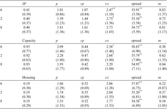
Table 1 reports the first 6, 12 and 18 step-ahead forecast error variances decompositions in income, prices, commodity prices, exchange rate, spread and money as the percentage of variances, which are attributable to spread.Table 2repeats the same exercise as the per-centage of variances, which are attributable to money rather than spread. It is first neces-sary to assess the impact of monetary policy (spread). Regarding the effect of monetary policy on income, it does not have a statistically significant impact on industrial produc-tion, capacity utilization rate or housing, which is parallel to Kim (1999) and Kim and Roubini (2000). Moreover, for the three income measures considered, there is no statisti-cally significant variation in prices accounted for by the spread. Importantly, a large var-iation of spread is also explained by itself. This supports the identification strategy, which assumes that the spread is exogenous and thus not explained by prices and output.

Table 1

How the spread explains each variable

IP p cp ex spread m 6 0.41 1.01 1.07 2.47** 55.91** 0.83 (0.39) (0.86) (0.84) (1.19) (5.58) (1.37) 12 0.40 1.59 1.44 2.75* 55.10** 0.75 (0.37) (1.23) (1.21) (1.56) (5.58) (1.25) 18 0.40 1.81 1.61 2.73 54.75** 0.81 (0.37) (1.36) (1.36) (1.65) (5.59) (1.17) Capacity p cp ex spread m 6 0.93 2.09 0.44 2.56* _58.85** _0.38 (0.77) (1.46) (0.67) (1.46) (6.90) (1.14) 12 0.92 2.28 0.47 2.66* _55.79** _0.62 (0.63) (1.80) (0.86) (1.80) (7.00) (1.33) 18 0.93 1.93 0.42 2.29 54.95** _0.84 (0.63) (1.77) (0.89) (1.80) (7.11) (1.40) Housing p cp ex spread m 6 0.19 1.66 0.52 2.06 57.87** _0.22 (0.30) (1.29) (0.69) (1.28) (6.75) (0.87) 12 0.19 1.74 0.55 2.04 55.20** 0.37 (0.30) (1.54) (0.89) (1.55) (6.81) (1.00) 18 0.19 1.53 0.52 1.77 54.58** 0.54 (0.29) (1.51) (0.93) (1.53) (6.89) (1.05)

Note: Standard errors are reported in parentheses under the corresponding coeﬃcients.

*

Indicates signiﬁcance at the 10% level.

**

(17)

The results that are obtained for money are considered in Table 2. The fraction of income (for all three income measures) and prices that are explained by the money aggre-gate are not statistically signiﬁcant. In addition, a large fraction of money is explained by money itself. However, as the time horizons increase, this fraction decreases.

An alternative approach to be followed in order to identify the monetary policy is to impose spread as an identifying assumption within structural VAR framework. This would allow the eﬀect of interbank interest rates on the macroeconomic performance to be observed.11 An attempt has been made to impose that constraint and estimate the model. When the constraints are imposed, the impulse response functions were not robust. A casual observation of the likelihood function suggests that a possible reason for unro-bustness was that local maximums were captured instead of the global maximum. 4. Conclusion

This paper proposes a measure of monetary policy for a highly inﬂationary, small and open economy. To be speciﬁc, innovations in the spread between the Central Bank’s inter-bank interest rate and the depreciation rate of the domestic currency are taken as an indi-cator of monetary policy. The empirical evidence suggests that a tight monetary policy,

Table 2

How money explains each variable

IP p cp ex spread m 6 2.91 0.71 0.40 0.44 0.71 86.79** (1.60) (0.84) (0.60) (0.58) (0.81) (4.86) 12 3.21 0.57 0.65 0.47 0.86 73.57** (1.80) (0.98) (1.25) (1.01) (0.90) (7.23) 18 3.19 0.31 0.88 0.53 0.89 62.09** (1.79) (0.47) (1.70) (1.27) (0.88) (7.51) Capacity p cp ex spread m 6 1.24 2.61 0.12 0.01 0.58 89.75** (1.59) (2.04) (0.43) (0.04) (0.82) (5.17) 12 1.32 2.50 0.12 0.04 0.66 81.41** (1.80) (2.74) (0.67) (0.34) (0.82) (6.61) 18 1.24 1.74 0.12 0.05 0.66 73.10** (1.69) (2.38) (0.75) (0.44) (0.81) (7.34) Housing p cp ex spread m 6 0.02 2.79 0.06 0.13 0.58 86.58** (0.16) (2.14) (0.31) (0.48) (0.79) (6.29) 12 0.08 2.63 0.09 0.21 0.60 78.49** (0.27) (2.79) (0.56) (0.88) (0.78) (7.63) 18 0.13 1.80 0.11 0.18 0.60 71.05** (0.30) (2.36) (0.71) (0.85) (0.77) (7.88)

Note: Standard errors are reported in parentheses under the corresponding coeﬃcients.

**_{Indicates signiﬁcance at the 5% level.}

11

See, for example, Cushman and Zha (1997). They imposed a real demand function as the identifying assumption where one could impose spread instead.

(18)

which is measured with positive innovation in spread, has a transitory effect on output, which drops for a short period of time in a statistically significant fashion. Moreover, the decrease in prices and appreciation of the local currency are permanent. Here, the qualitative inferences concerning the effect of monetary policy are on parallel with the dif-ferent specification models used in the previous studies (seeSims, 1992; Eichenbaum and Evans, 1995; Grilli and Roubini, 1995; Kim and Roubini, 2000).

The recursive system used in this paper produced impulse response functions that are not inconsistent with widely accepted views on the qualitative impact of a monetary policy shock on various macroeconomic variables. The absence of the price, liquidity and exchange rate puzzles discussed in the previous section also suggests that the proposed macroeconomic variable used here as an indicator of monetary policy and the recursive identiﬁcation scheme are not at odds with economic theories.

This paper imposes additional importance on the identiﬁcation of monetary policy for a small open economy. Policy makers from small open economies have additional challenges that are not present in developed economies, such as the threat of currency substitution or the level of foreign exchange rate reserves. Hence, identifying the spread as an indicator of monetary policy for Turkey suggests the interesting possibility that the same variable could be used as an indicator of monetary policy for other small open economies.

There are several issues which are not addressed here. The inclusion of ﬁscal policy could produce a more complete picture of the behavior of prices and output. There are some periods when the CBRT used money aggregate targeting (January 1998–June 1998) and periods that targeted Net Domestic Assets (July 1998–November 2000). Fur-thermore, the behavior of the Foreign Reserves of the CBRT is not modeled. The level and behavior of foreign exchange reserves are important and closely monitored by the public and the CBRT. These are areas to be dealt with in future research.

Acknowledgement

I thank Anita Akkasß, Emre Alper, Sßu¨ku¨ Binay, Haluk Erlat, Richard Froyen, Kamu-ran Malatyalı, participants of seminars at Bosphorus and Middle East Technical Univer-sities and three anonymous referees for their helpful comments.

References

Agenor, P-R., Montiel, P., 1999. Development Macroeconomics, Second ed. Princeton University Press, Princeton, NJ.

Alper, E., Onis, Z., 2003. Financial globalization, the democratic deﬁcit and recurrent crises in emerging markets: The Turkish experience in the aftermath of capital account liberalization. Emerging Markets Finance and Trade 39 (3), 5–26.

Aslanoglu, Erhan, 2001, Shrinkage in economy (in Turkish), http://www.ntvmsnbc.com/news/ 79366.asp?0m=S1412001.

Barro, R.J., 1977. Unanticipated money growth and unemployment in the United States. American Economic Review 67 (2), 101–115.

Bernanke, B., 1983. Nonmonetary eﬀects of the ﬁnancial crisis in the propagation of the great depression. American Economic Review 73 (3), 257–276.

Bernanke, B., 1990. On the predictive power of interest rates and interest rates, New England Economic Review. Federal Reserve Bank of Boston 73 (3), 51–68.

Bernanke, B., Blinder, A., 1992. Federal funds rate and the channels of monetary transmission. American Economic Review 82 (4), 901–921.

(19)

Bernanke, B., Mihov, I., 1998. Measuring monetary policy. Quarterly Journal of Economics 113 (3), 869–902. Berument, H., Neyapti, B., 1999. How independent is the Central Bank of the Republic of Turkey (in Turkish).

Iktisat, Isletme ve Finans 165, 11–17.

Christiano, L., Eichenbaum, M., Evans, C.L., 1996a. The eﬀect of monetary policy shocks: Evidence from the ﬂow of funds. Review of Economics and Statistics 78 (1), 16–34.

Christiano, L., Eichenbaum, M., Evans, C.L., 1996b. Implication and the eﬀects of monetary policy shocks. In: Blejer, M. (Ed.), Financial Factors in Economic Stabilization and Growth. Cambridge University Press, New York, pp. 36–74.

Christiano, L., Eichenbaum, M., Evans, C.L., 1999. Monetary policy shocks: What have we learned and to what end? In: Taylor, J.B., Woodford, M. (Eds.), In: Handbook of Macroeconomics, vol 1A. North-Holland, Amsterdam, pp. 65–148.

Cushman, D.O., Zha, T., 1997. Identifying monetary policy in a small open economy under ﬂexible exchange rates. Journal of Monetary Economics 39, 433–448.

Doan, T.A., 2000, RATS version 5, Estima, Cambridge, MA.

Eichenbaum, M., Evans, C.L., 1995. Some empirical evidence on the eﬀect of shock to monetary policy on exchange rates. Quarterly Journal of Economics 110, 975–1009.

Ergun, M., 2000. Electoral political business cycles in Turkey. Russian and East European Finance and Trade Journal 36 (6), 6–32.

Ertugrul, A., Selcuk, F., 2002. Turkish economy: 1980–2001. In: Kibritcioglu, A., Rittenberg, L., Selcuk, F. (Eds.), Inﬂation and Disinﬂation in Turkey. Ashgate, Hampshire, England, pp. 13–40.

Friedman, B.M., Kuttner, K.N., 1992. Money, income, prices and interest rates. American Economic Review 82 (3), 472–492.

Fuhrer, J.C., Moore, G.R., 1995a. Inﬂation persistence. Quarterly Journal of Economics 110 (1), 127–159. Fuhrer, J.C., Moore, G.R., 1995b. Monetary policy trade-oﬀs and the correlation between nominal interest rates

and real output. American Economic Review 85 (1), 219–239.

Geweke, J.F., Runkle, D.E., 1995. A ﬁne time for monetary policy? Federal Reserve Bank of Minneapolis Quarterly Review 19 (1), 18–31.

Gokce, D., 2001, The old program died. Will the new program be diﬀerent (in Turkish), Aksam, 02,27,2001,

http://www.aksam.com.tr/arsiv/aksam/2001/02/27/yazarlar/yazarlar30.html.

Grilli, V and Roubini, N. 1995. Liquidity and exchange rates: Puzzling evidence from the G-7 countries, Working Paper, Yale University, CT.

ISO, 2002, The 500 Largest Industrial Establishments. Istanbul Industry Organization, Istanbul (in Turkish). Kim, S., 1999. Do monetary policy shocks matter in the G-7 countries? Using common identifying assumptions

about monetary policy across countries. Journal of International Economics 48, 387–412.

Kim, S., Roubini, N., 2000. Exchange rate anomalies in industrial countries: A solution with a structural VAR approach. Journal of Monetary Economics 45, 561–586.

Koray, F., McMillin, W.D., 1999. Monetary shocks, the exchange rate, and the trade balance. Journal of International Money and Finance 18, 925–940.

Leeper, E.M., Gordon, D.B., 1992. In search of the liquidity eﬀect. Journal of Monetary Economics 29 (3), 341– 369.

Litterman, R.B., Weiss, L., 1985. Money, interest rates, and output: A Reinterpretation of postwar US data. Econometrica 53, 129–156.

Mishkin, F.S., 1983. A Rational Expectation Approach to Testing Macroeconomics: Testing Policy Ineﬀective-ness and Eﬃcient-Market Models. University of Chicago Press, Chicago, IL.

Mosconi, R., 1998, MALCOLM (MAximum Likelihood CO integration analysis of Linear Models (Cafoscarina, Venezia, Italy).

Ozatay, F., 2000. The 1994 currency crisis in Turkey. Journal of Policy Reform 3 (4), 327–352.

Sayan, S., Berument, H., 1997. Politics in Turkey, economic populism and governments (in Turkish). H.U. Iktisadi ve Idari Bilimler Fakultesi Dergisi 15 (2), 171–185.

Sims, C., 1980. Comparison of interwar and postwar business cycles: Monetarism reconsidered. American Economic Review Papers and Proceedings 70, 250–257.

Sims, C.A., 1986. Are forecasting models usable for policy analysis? Federal Reserve Bank of Minneapolis Quarterly Review 10 (1), 2–16.

Sims, C.A., 1992. Interpreting the macroeconomic time series facts. European Economic Review 36, 975–1011. Sims, C.A. and Zha, T. 1996. Does monetary policy generate recession? Mimeo.

(20)

Strongin, S., 1995. The identiﬁcation of monetary policy disturbances explaining the liquidity puzzle. Journal of Monetary Economics 35, 463–497.

VII. Demirel Government Coalition Protocol (in Turkish), 1991.

Walsh, C.E., 1998. Monetary theory and policy. MIT Press, Armonk, NY.

Yildiz, Huseyin I., 2002, The past and future of banking (2) (in Turksih), Aksam, 09,28,2002, http:// www.aksam.com.tr/arsiv/aksam/2002/09/28/yazarlar/yazarlar4.html.