A local search heuristic with self-tuning parameter for permutation flow-shop scheduling problem

Abstract—In this paper, a new local search metaheuristic is proposed for the permutation flow-shop scheduling problem. In general, metaheuristics are widely used to solve this problem due to its NP-completeness. Although these heuristics are quite effective to solve the problem, they suffer from the need to optimize parameters. The proposed heuristic, named STLS, has a single self-tuning parameter which is calculated and updated dynamically based on both the response surface information of the problem field and the performance measure of the method throughout the search process. Especially, application simplicity of the algorithm is attractive for the users. Results of the experimental study show that STLS generates high quality solutions and outperforms the basic tabu search, simulated annealing, and record-to-record travel algorithms which are well-known local search based metaheuristics.

I. INTRODUCTION

HIS paper deals with the permutation flow-shop scheduling problem (PFSP) to minimize makespan which generally arises in industrial processes. There are n jobs to be processed in the same sequence on m machines. Processing time of job i on machine j is represented by tij≥ 0.

It is assumed that machines can process at most one job at a time and the operating sequences of the jobs are the same on every machine. The processing of a given job at a machine also cannot be interrupted. PFSP with makespan criterion can be denoted as F/prmu/Cmax following the notation given by Graham et al. [1]. Maximum completion time, Cmax, is the time at which the last job in the sequence is completed at the last machine, m. The problem is to determine the best operating sequence of the jobs which minimizes the makespan or Cmax. PFSP is known to be NP-complete for more than two machines (Garey et al. [2]). Although a number of exact approaches have been suggested (for example Johnson [3], Lomnicki [4]), most of the literature in the last years recommends the metaheuristic procedures in order to obtain near-optimal solutions for the problem. Recent reviews of PFSP literature are given by Framinan et al. [5], Ruiz and Maroto [6], Hejazi and Saghafian [7]. Metaheuristic approaches are generally viewed as effective for large sized PFSP in the literature, as they are successful

to solve other combinatorial optimization problems.

Since the metaheuristics are controlled by a set of parameters, a typical application of these heuristics requires a crucial task known as parameter optimization, parameter tuning or parameter setting. A careful selection of the best set of parameter values requires either a deep knowledge of the problem structure or a lengthy trial-and-error process. The best parameter set is usually re-determined before the running considering size or input data of the each individual problem. Tuning a metaheuristic’s parameters to produce robustness and effectiveness is a tedious and time-consuming process. Adenso-Diaz and Laguna [8] state that about 10% of the total time dedicated to designing and testing of a new heuristic is spent for development, and the remaining 90% is consumed for fine-tuning of parameters.

An alternative way to tuning parameters before the run is to control of these parameters through the run. Heuristics of this nature are generally called adaptive, reactive or self-tuning heuristics. In this paper a modification of local search heuristic with a single self-tuning parameter, Ө, is presented. Ө is obtained and updated dynamically throughout the search process. The effectiveness of the self-tuning local search (STLS) heuristic is improved using the response surface information which comes from the problem instance and the performance measure of the algorithm. The most important advantage of STLS is that the algorithm does not need additional time and specialization to manage parameter optimization.

The rest of this paper is organized as follows. Section II explains the STLS. Implementations of STLS, tabu search (TS), simulated annealing (SA), and record-to-record travel (RRT) heuristics for PFSP are given in Section III. The section of computational study includes the comparison of STLS with the TS, SA, and RRT algorithms. Finally, the last section presents the conclusions.

II. DESCRIPTION OF STLS

STLS algorithm starts with any initial solution

X

_z as a current solution and searches the solution space iteratively. X represents the vector [x1, x2, …, xn] which corresponds the

A Local Search Heuristic with Self-tuning Parameter for

Permutation Flow-Shop Scheduling Problem

Berna Dengiz

a

_{, Cigdem Alabas-Uslu}

b

_{, and Ihsan Sabuncuoglu}

c a

Department of Industrial Engineering, Baskent University, 06530, Ankara, Turkey

b

_{Department of Industrial Engineering, Maltepe University, 34857, Istanbul, Turkey}

c

_{Department of Industrial Engineering, Bilkent University, 06800, Ankara, Turkey}

T

operating sequence of jobs such that xj is the job placed in j.

order. At iteration i, a neighbor solution X' selected randomly from the neighborhood of the current solution X. X' is accepted as the new current solution if the following condition is satisfied:

If f(X') ≤ Өf(X) then X ← X'

Here, f(X) is the maximum completion time, Cmax, of the current solution X at iteration i. Ө is the self-tuning parameter of STLS. The algorithm progresses to the next iteration when an acceptable solution is obtained. Otherwise, a new neighbor solution is selected randomly from the neighborhood. If the total number of rejected neighbors reaches the neighborhood size of the current solution, ⏐N(X)⏐, respect to the moving mechanism under consideration, value of Ө is increased using the equation Ө = Ө + α1α2. The sampling of neighbors is implemented with replacement to avoid excessive consumption of computer memory. Search process around the current solution X is repeated to obtain an acceptable neighbor solution.

Dynamic calculation of parameter Ө is based on two criteria: the number of improved solutions obtained during the search process and the quality of these solutions relative to the initial solution. Hence, the measures given by equations 1-2 are introduced, where

X

(i_b) is the best solution observed until iteration i,

X

_z is the initial solution, C(L(i)_{) is the number of improved solutions obtained until} iteration i:

)

(

)

(

() 1 z i b

f

f

X

X

=

α

(1)

i

i

₎

L

(

C

() 2

=

α

(2)

C(L(i)_{) is calculated as C(L}(i)_{) = C(L}(i)_{) + 1, if f(X') <}

)

(

(i)

b

f X

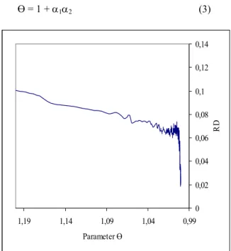
for an accepted neighbor solution X'. STLS assumes that f(X) > 0, for the whole solution space. Finally, parameter Ө is computed during the search by the equation 3. In this way, the parameter determine the borders of the search region around the current solution X taking into account the number of improved solutions and the solution quality. During the initial iterations of the algorithm, the search is almost random. It is expected that while Ө approaches to 1, the search is forced to find better solutions. For instance, Figure 1 depicts the decrease of relative deviation from the best known solution (RD) accompanied by parameter Ө. Furthermore, changing of parameter Ө with respect to the number of iterations is shown in Figure 2. As seen from the figure, Ө exponentially decreases as the number of iterations increases.

Ө = 1 + α1α2 (3) 0 0,02 0,04 0,06 0,08 0,1 0,12 0,14 0,99 1,04 1,09 1,14 1,19 Parameter Ө RD

Fig. 1. Improvement of solution quality according to Ө for a 200n/20m PFSP

An experimental study is undertaken to show the effectiveness of the dynamic calculations of Ө comparing with the fixed values for Ө. Three fixed levels, 1.0015, 1.0025, and 1.0035, which have generated reasonably good results in preliminary experiments, are selected for Ө. These fixed levels and dynamic calculation of Ө are tested on selected three problems from the whole benchmark set of Taillard [13]. Table I shows the average deviations from the best known solutions over the 10 runs for the test problems. As seen from the table dynamic Ө generates higher qualified solutions than the fixed Ө values for the each size, except fixed value 1.0015. Ө = 1.0015 cause 0.0095 deviation from the best known while dynamic Ө yields 0.0101 for 50/20 sized problem. However, the self-tuning of Ө outperforms the manually controlling of Ө according to the average results for the all problem sizes.

1 1,0005 1,001 1,0015 1,002 1,0025 1,003 0 200000 400000 600000 800000 1000000 1200000 1400000 Number of iterations Ө

III. IMPLEMENTATION

STLS algorithm is compared with some widely used local search based metaheuristics: TS (Glover [9]), SA (Kirkpatrick et al. [10]), and RRT (Dueck [11]). Details of these metaheuristics can be found in the last mentioned references. There are also many sophisticated metaheuristics proposed in PFSP literature. However, the aim of this study is to examine the effectiveness and efficiency of STLS relative to the standard versions of TS, SA and RRT metaheuristics, since STLS also relies on a simple principle. In this study, TS, SA, and RRT algorithms are coded sticking to the basic principles proposed by the pioneers employing the same neighbor generation mechanism with STLS. Thus, they run under the same base line. Basic structures and acceptance conditions of STLS, TS, SA, and RRT algorithms are defined in the subsection B.

A. Neighbor Generation

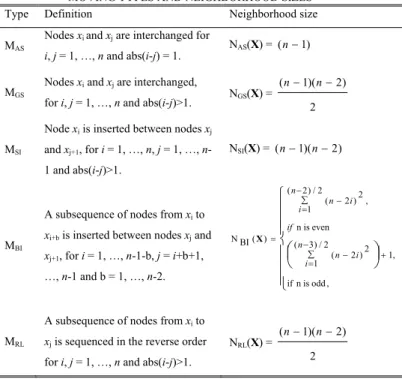
Neighborhood of a solution point X is created using five different moving types: Adjacent swap (MAS), general swap (MGS), single insertion (MSI), block insertion (MBI) and reverse location (MRL). These moving types are the most commonly used types of perturbation schemes for generating neighbor solutions and an analysis of them can be found in Tian et al. [12] for a SA algorithm. The definitions of the moves and neighborhood sizes obtained by these moves are given in Table II.

TABLE II

MOVING TYPES AND NEIGHBORHOOD SIZES Type Definition Neighborhood size MAS

Nodes xi and xj are interchanged for

i, j = 1, …, n and abs(i-j) = 1. NAS(X) = (n−1)

MGS

Nodes xi and xj are interchanged,

for i, j = 1, …, n and abs(i-j)>1. NGS(X) = ₂ ) 2 )( 1 (n− n− MSI

Node xi is inserted between nodes xj

and xj+1, for i = 1, …, n, j = 1, …,

n-1 and abs(i-j)>n-1.

NSI(X) = (n−1)(n−2)

MBI

A subsequence of nodes from xi to

xi+b is inserted between nodes xj and

xj+1, for i = 1, …, n-1-b, j = i+b+1,

…, n-1 and b = 1, …, n-2.

MRL

A subsequence of nodes from xi to

xj is sequenced in the reverse order

for i, j = 1, …, n and abs(i-j)>1.

NRL(X) = 2 ) 2 )( 1 (n− n−

B. Structures and Acceptance Conditions of the Algorithms

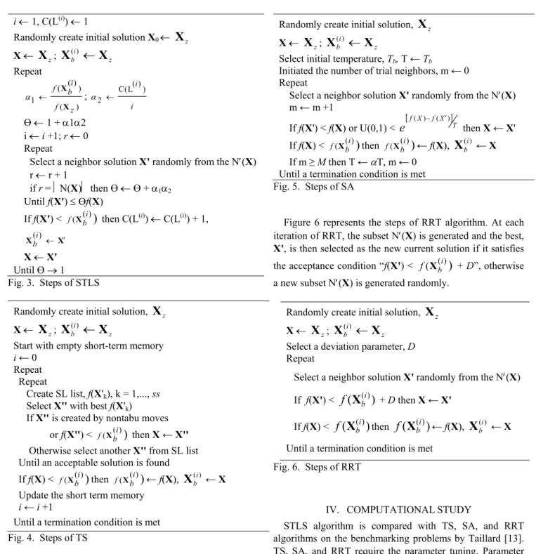
Implementation steps of STLS algorithm are given in Figure 3. At each iteration of the algorithm, a subset N′(X: X(s) _{, s =1, …, 5), is generated by applying the five different} moving types to the current solution X. The best one, X', among these neighbors with best objective value is then selected as a new current solution if it satisfies the acceptance condition “f(X') ≤ Өf(X)”, otherwise a new subset N′(X) is generated randomly.

Steps of TS are shown in Figure 4. TS uses a short-term memory with size tt. If the current solution has been created by adjoining job p and r, moves which disarrange this successive subsequence of the job p and r are classified as tabu during next tt iterations. At each iteration, the subset N′(X: X(s) _{, s =1, …, 5) is obtained and the best solution in} the subset which created using a non-tabu move, X', is added to a sampling list, SL, with size ss. If the N′ entirely contains tabu moves, then a new N′ is generated until SL is filled with ss solutions. However, the aspiration criterion removes the tabu condition when any move yields a better solution than the best solution obtained so far. The best solution, X'', in the sampling list is accepted as the new current solution.

TABLE I

AVERAGE DEVIATION FROM THE BEST KNOWN USING FIXED AND DYNAMIC θ n/m Ө 1.0015 1.0025 1.0035 Dynamic 50/20 0.0095 0.0276 0.0374 0.0101 100/20 0.0254 0.0371 0.0427 0.0016 200/20 0.0328 0.0387 0.0425 0.0018 Average 0.0226 0.0345 0.0409 0.0045 ⎪ ⎪ ⎪ ⎩ ⎪⎪ ⎪ ⎨ ⎧ ⎟ ⎠ ⎞ ⎜ ⎝ ⎛ −_{∑ +} = − ∑ − = − = , odd is n if , 1 2 / ) 3 ( 1 2 ) 2 ( even is n 2 / ) 2 ( 1 , 2 ) 2 ( ) ( BI N n i n i if n i n i X

i ← 1, C(L(i)_{) ← 1}

Randomly create initial solution X0 ←

X

_z

X ←

X

_z;

X

_b(i)

←

X

_z Repeat ) ( ) ) ( ( 1 z f i b f X X ← α ; i i ) ) ( L ( C 2 ← α Ө ← 1 + α1α2 i ← i +1; r ← 0 Repeat

Select a neighbor solution X' randomly from the N′(X) r ← r + 1

if r = ⏐N(X)⏐ then Ө ← Ө + α1α2 Until f(X') ≤ Өf(X)

If f(X') < f X( (_bi)

)

then C(L(i)_{) ← C(L}(i)_{) + 1,}

X X(i_b) ← ′ X ← X' Until Ө → 1 Fig. 3. Steps of STLS

Randomly create initial solution,

X

_z X ←

X

_z;

X

_b(i)

←

X

_z

Start with empty short-term memory i ← 0

Repeat Repeat

Create SL list, f(X'k), k = 1,..., ss Select X'' with best f(X'k)

If X'' is created by nontabu moves or f(X'') < f X( (_bi)

)

then X ← X''

Otherwise select another X'' from SL list Until an acceptable solution is found

If f(X) < f X( (_bi)

)

then f X( _b(i)

)

← f(X),

X

(i_b) ← X Update the short term memory

i ← i +1

Until a termination condition is met Fig. 4. Steps of TS

The SA algorithm is given in Figure 5. The best solution, X', in the N′(X) is recorded as the current solution, if f(X') < f(X) or U(0,1) <

_e

[f(X)−f(X′)]T _{is satisfied, where U(0,1)}

represents a uniformly generated number between 0 and 1. T is a control parameter. The algorithm proceeds by attempting a certain number of neighborhood moves, M, at each temperature, while T is gradually dropped in the ratio of α.

Randomly create initial solution,

X

_z X ←

X

_z;

X

_b(i)

←

X

_z

Select initial temperature, Tb, T ← Tb

Initiated the number of trial neighbors, m ← 0 Repeat

Select a neighbor solution X' randomly from the N′(X) m ← m +1

If f(X') < f(X) or U(0,1) <

_e

[f(X)−f(X′)]T _{then X ← X'}

If f(X) < f X( (_bi)

)

then f X( _b(i)

)

← f(X),

X

(i_b) ← X If m ≥ M then T ← αT, m ← 0

Until a termination condition is met Fig. 5. Steps of SA

Figure 6 represents the steps of RRT algorithm. At each iteration of RRT, the subset N′(X) is generated and the best, X', is then selected as the new current solution if it satisfies the acceptance condition “f(X') < f X( (_bi)

)

+ D”, otherwise a new subset N′(X) is generated randomly.

Randomly create initial solution,

X

_z X ←

X

_z;

X

_b(i)

←

X

_z

Select a deviation parameter, D Repeat

Select a neighbor solution X' randomly from the N′(X) If f(X') <

f X

(

(i_b)

)

+ D then X ← X'

If f(X) <

f X

(

(i_b)

)

then

f X

(

_b(i)

)

← f(X),

X

_b(i) ← X Until a termination condition is met

Fig. 6. Steps of RRT

IV. COMPUTATIONAL STUDY

STLS algorithm is compared with TS, SA, and RRT algorithms on the benchmarking problems by Taillard [13]. TS, SA, and RRT require the parameter tuning. Parameter selection studies for these algorithms are given in the next subsection.

A. Parameter Selection

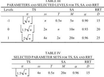
The basic TS, SA, and RRT algorithms have parameter sets which shown in Table III. These parameter sets must be tuned for each algorithm before the run. 3k _factorial experiments designed for this purpose, where k is the number of parameters of the related algorithm (k is equal to 2, 3, and 1 for TS, SA, and RRT, respectively). Table III

also shows the selected parameter levels based on pre-examinations for the factorial designs. Three separate factorial designs were carried out for the each algorithm taking into account the same statistical method. The algorithm under consideration was run 5 times for each of the parameter combinations and then an analysis of variance using confidence level as 95% was performed. Results of the statistical analysis show that the parameters are statistically significant and solution quality of the related algorithm is influenced by the parameter levels. Consequently, the best parameter sets which cause the best solution quality are selected as given in Table IV.

STLS algorithm has a single parameter Ө and this parameter is tuned throughout the run, as explained before. STLS is distinguished from the other algorithms since it does not need any parameter optimization effort.

B. Comparison Results

30 particular hard instances of 3 different sizes are selected from the whole benchmark set of Taillard [13], since global optima are known for the smaller instances. A sample of 10 instances is provided for each of 50/20, 100/20, and 200/20 (n/m) sizes.

STLS, TS, SA, and RRT algorithms were executed 20 times on a Pentium IV/1000-512 RAM computer. All the algorithms were terminated when the number of searched solutions reaches the same maximum level. Following performance measures were obtained at the end of this experimental study: Relative Deviation:

=

−

j=_{1 K}, ,20 O O O RD _B B A j j

Where,

O

A_j is the objective value of the considered algorithm obtained from replication j. _{O is the best known} B objective value which taken from [14].

Best Relative Deviation: BRD =

( )

RD_j j min

Average Relative Deviation: ARD = 20 ∑ j RDj Coefficient of Variation: CV =

[

]

ARD ARD RD j 1 j 20 2 ∑ − =

Average Run Time in Minutes: ART = 20 ∑

j Runtimej

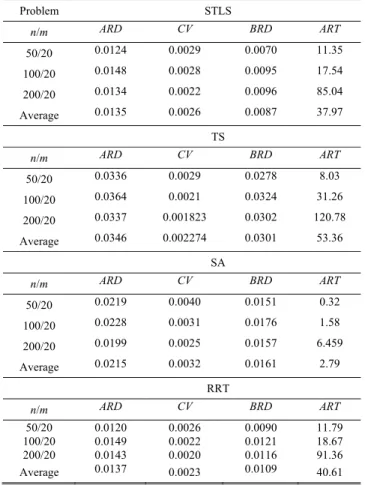
Performances of the algorithms are displayed in Table V. As seen from the table, STLS algorithm generates lower ARD and BRD values than the other algorithms for the each problem size, except the size 50/20. RRT yields better solution quality than STLS for this size in terms of ARD. In the average case, the solution quality of RRT algorithm is close to performance of STLS. CV values of the all algorithms are found as close to each other. However all the algorithms run considering the same maximum level of searched solutions, their average run times are found different from each other. TS is the slowest algorithm as well as it has the worst solution quality. The sampling list of TS must be fielded by non-tabu solutions as expressed in Section III. This situation causes the slowest average run time for TS. ART value of RRT is obtained higher than STLS only 2.64 minutes. This difference arises from the change in the acceptance conditions of STLS and RRT. While the acceptance condition of RRT is based on the objective value of best solution, f X( (i_b)), this condition relies on the objective value of current solution, f(X), for STLS, as explained in Section III. On the other hand, SA algorithm replaces any trial solution with the current solution if the trial satisfies the acceptance condition of SA and the algorithm proceeds to the next iteration even the trial solution is not accepted. However, STLS, TS, and RRT algorithms force the search to find an acceptable solution. Therefore, SA is found as the fastest algorithm as seen from Table V. Despite the fact that SA has minimum ART, it should be recalled that parameter optimization of SA consumed a certain amount of computer times at the beginning of the study. Table VI also shows the absolute BRD and ARD differences between STLS and the other algorithms. Accordingly, STLS algorithm generates 0.0214, 0.0074, and 0.0022 less average BRD values than TS, SA, and RRT algorithms, respectively.

Figure 7 shows convergences of the algorithms for a 100/20 sized PFSP. STLS converges to higher quality solutions searching more number of solutions than the other algorithms search.

TABLE IV

SELECTED PARAMETER SETS FOR TS, SA AND RRT

TS SA RRT

tt ss T M α D

⎣ ⎦

1.5 n 4n 0.5n 20n 0.96 15 TABLE III

PARAMETERS AND SELECTED LEVELS FOR TS, SA AND RRT

Levels TS SA RRT

tt ss T M α D

-1

⎣ ⎦

n n 0.5n 5n 0.90 15

0

⎣ ⎦

1.5 n 2n n 10n 0.93 20

V. CONCLUSION

This paper presents a modified local search algorithm with a single tuning parameter for PFSP. The self-tuning parameter of the STLS algorithm is obtained and updated dynamically throughout the search process to improve the effectiveness of the algorithm. The most important advantage of STLS is that the algorithm does not need additional computational efforts for parameter optimization. This simplicity enables the users to employ the algorithm for solving of different PFSP cases easily.

STLS also provides high quality solutions to the well-known benchmark problems when compared with the basic forms of TS, SA, and RRT algorithms. Furthermore, obtained solutions by STLS solely deviate 0.87% from the best-known solutions which are generally generated by sophisticated metaheuristics in the PFSP literature.

Improvements on STLS to obtain higher quality solutions to PFSP spending less run time will be examined in the future study.

REFERENCES

[1] R.L. Graham, E.L. Lawler, J.K. Lenstra, and A.H.G. Rinnooy Kan, “Optimization and approximation in deterministic sequencing and scheduling: A survey”, Annals of Discrete Mathematics, 1979, vol. 5, pp. 287–326.

[2] M.R. Garey, D.S Johnson,. and R. Sethi, “The Complexity of Flow-Shop and Job-Flow-Shop Scheduling, Mathematics of Operations

Research”, 1976, vol. 1, pp. 117-129.

[3] S.M. Johnson, “Optimal two- and three-stage production schedules”,

Naval Research Logistics Quarterly, 1954, vol. 1, pp. 61-68.

[4] Z.A. Lomnicki, “A branch-and-bound algorithm for the exact solution of the three-machine scheduling problem”, Operations Research. Quarterly, 1965, vol. 16, pp. 89–100.

[5] J.M. Framinan, J.N.D Gupta, and R. Leisten, “A review and classification of heuristics for permutation flow-shop scheduling with makespan objective”, Journal of the Operational Research

Society,2004, vol. 5, pp. 1243–1255.

[6] R. Ruiz, and C. Maroto, “A comprehensive review and evaluation of permutation flowshop heuristics”, European Journal of Operational

Research, 2005, vol. 165, pp. 479-494.

[7] S.R. Hejazi, and S. Saghafian, S, “Flowshop-scheduling problems with makespan criterion: a review”, International Journal of

Production Research, 2005, vol. 43(14), pp. 2895–2929.

[8] B. Adenso-Diaz and M. Laguna, “Fine-tuning of algorithms using fractional experimental designs and local search”, Operations

Research, 2006, vol. 54 (1), pp. 99-114.

[9] F. Glover, “Future paths for integer programming and links to artificial intelligence”, Computers & Operations Research, 1986, vol. 1(3), pp. 533-549.

[10] S. Kirkpatrick, C.D. Gelatt Jr. and M.P. Vecchi, “Optimization by simulated annealing”, Science, 1983, vol. 220(4598), pp. 671-680. [11] G. Dueck, “New optimization heuristics: The great deluge algorithm

and the record-to-record travel”, Journal of Computational

Physics,1993, vol. 104, pp. 86-92.

[12] P. Tian, J. Ma and D-M. Zhang,. “Application of the simulated annealing algorithm to the combinatorial optimization problem with permutation property: An investigation of generation mechanism”,

European Journal of Operational Research, 1999, vol. 118, pp. 81-94.

[13] E. Taillard, “Some efficient heuristic methods for the flow shop sequencing problem”, European Journal of Operational Research, 1990, vol. 47(1), pp. 65-74.

[14] Available: http://mistic.heig-vd.ch/taillard/ TABLE VI

PROVIDED IMPROVEMENTS ON TS, SA, RRT

Performance TS SA RRT

BRD 0.0214 0.0074 0.0022

ARD 0.0211 0.0080 0.0002

TABLE V

PERFORMANCE COMPARION OF THE ALGORITHMS

Problem STLS n/m ARD CV BRD ART 50/20 0.0124 0.0029 0.0070 11.35 100/20 0.0148 0.0028 0.0095 17.54 200/20 0.0134 0.0022 0.0096 85.04 Average 0.0135 0.0026 0.0087 37.97 TS n/m ARD CV BRD ART 50/20 0.0336 0.0029 0.0278 8.03 100/20 0.0364 0.0021 0.0324 31.26 200/20 0.0337 0.001823 0.0302 120.78 Average 0.0346 0.002274 0.0301 53.36 SA n/m ARD CV BRD ART 50/20 0.0219 0.0040 0.0151 0.32 100/20 0.0228 0.0031 0.0176 1.58 200/20 0.0199 0.0025 0.0157 6.459 Average 0.0215 0.0032 0.0161 2.79 RRT n/m ARD CV BRD ART 50/20 0.0120 0.0026 0.0090 11.79 100/20 0.0149 0.0022 0.0121 18.67 200/20 0.0143 0.0020 0.0116 91.36 Average 0.0137 0.0023 0.0109 40.61 -0,01 0,01 0,03 0,05 0,07 0,09 0,11 0,13 0,15 0 1000000 2000000 3000000 4000000 5000000 6000000 number of solutions searched

RD

STLS TS SA RRT