Once burned, twice shy: money market fund responses to a systemic liquidity shock

(1)

doi:10.1017/S0022109015000101

Once Burned, Twice Shy: Money Market Fund

Responses to a Systemic Liquidity Shock

Philip E. Strahan and Ba¸sak Tanyeri

∗

Abstract

After Lehman’s collapse in 2008, investors ran from risky money market funds. In 27 funds, outflows overwhelmed cash inflows, thus forcing asset sales. These funds sold their safest and most liquid holdings. Funds were thus left with riskier and longer maturity assets. Over the subsequent quarter, however, the hard-hit funds reduced risk more than other funds. In contrast, money funds hit by idiosyncratic liquidity shocks before Lehman did not alter portfolio risk. The result suggests that moral hazard concerns with the Treasury Guarantee of investor claims did not increase risk taking. Funds that benefited most from the government bailout reduced risk.

I. Introduction

This article studies how money market fund portfolios changed after the run that followed the bankruptcy of Lehman Brothers on Sept. 15, 2008. We focus on how money funds met withdrawal demands through portfolio reallocations in both the short run and the long run. Funds hardest hit by investor runs reacted initially by meeting withdrawal demands with cash generated from maturing assets and by selling off the safest and most liquid holdings. As a result, immediately after the run ended, hard-hit funds had increased portfolio risk and lengthened asset maturity relative to other funds. By the end of 2008, however, these hard-hit funds had reallocated their investments to safer and shorter term investments than what they had held on the eve of the crisis.

Consistent with other research (McCabe (2010), Kacperczyk and Schnabl (2013)), we start by showing that fund flows responded rationally to the sharp change in expectations about the risks of commercial paper investments. Due to its large exposure to Lehman Brothers’ commercial paper, the Reserve Primary Fund “broke the buck” on Sept. 16, 2008. This announcement initiated a run across the money market industry, whereby institutional investors withdrew funds en masse from risky prime funds (a major holder of commercial paper) and, in aggregate,

∗_{Strahan (corresponding author), [email protected], Carroll School of Management, Boston}

College, Chestnut Hill, MA 02467; Tanyeri, [email protected], Faculty of Business Administra-tion, Bilkent University, Ankara 06800, Turkey. We thank an anonymous referee, Stephen Brown (the editor), Philipp Schnabl, and seminar participants at Boston College and Bilkent University for helpful comments.

119

https://www.cambridge.org/core

. Bilkent University Library

, on

25 Aug 2017 at 13:17:02

, subject to the Cambridge Core terms of use, available at

https://www.cambridge.org/core/terms

(2)

reallocated their investments to safer funds holding mainly U.S. government se-curities and repurchase agreements (repos). Retail investors also withdrew from risky funds, but on a somewhat smaller scale than institutional investors. Cross-sectional regressions suggest that funds most heavily invested in risky assets, such as commercial paper, faced the largest outflows.

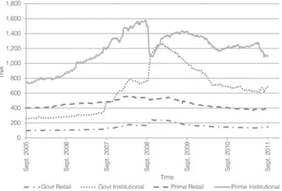
Figure 1 graphs the evolution of total net assets (TNA) in the mutual fund business over time. The figure separates the data into four groups based on the fund’s main asset class and investor type: prime-institutional, prime-retail, government-institutional, and government-retail. First, the figure shows that in-stitutional investors dominate TNA and aggregate flows in the industry. Second, the figure shows a dramatic reallocation of total investment from the prime (risky) to the government (safe) funds. Figure 2 shows the percentage change in TNA during the days surrounding the Lehman collapse: just before (Sept. 9–12), during (Sept. 15–19), and after (Sept. 22–23), again separated by clientele and investment strategy.

We focus on how funds adjusted their positions in response to these large flows. In general, funds facing liquidity pressure can minimize short-run costs first by using cash from maturing assets to pay claims, and second by selling their most liquid (and safe) nonmaturing assets before selling less liquid (and less safe) assets. Because such a strategy leaves the fund holding riskier and less liquid assets than before the shock, however, long-run stability could be jeopardized by continued outflows. Hence, a fund facing outflows that it fears may continue could instead opt to sell some of its less liquid positions to maintain a liquidity buffer to insure against continued outflows. We find strong evidence consistent with the first strategy. This behavior likely reflects, first, the reality that selling risky holdings such as commercial paper became all but impossible in the days

FIGURE 1

Aggregate TNA by Category (billions of $)

Figure 1 reports the time series of aggregate total net assets (TNA) held by money market mutual funds from Sept. 2005 to the end of 2011 for the four segments of the money market mutual fund industry.

, on

25 Aug 2017 at 13:17:02

(3)

FIGURE 2

Flow as Percentage of TNA during the Days Surrounding Lehman’s 2008 Bankruptcy

Figure 2 reports the daily percentage change in aggregate TNA during the days just before and just after the Lehman bankruptcy (Sept. 15, 2008) for the four segments of the money market mutual fund industry.

following the Lehman bankruptcy. Most potential buyers would have been other prime funds, which themselves faced liquidity pressures. Second, the rapid initia-tion of government protecinitia-tion provided to investors obviated concerns about long-run viability for liquidity-stressed funds. The U.S. Treasury provided an ex post, across-the-board guarantee against breaking the buck for all money market funds on Sept. 19, 2008 (excluding the Reserve Primary Fund, which had already broken the buck). As should be clear from Figure 2, this policy action stopped the run after just 4 days. The Treasury program was available to all money funds for 1 basis point per dollar of net asset value. We find that funds more exposed to outflows and holding a greater share of high-risk, high-yield assets were more likely to enter the program.

We then test whether mutual funds made long-run changes to their portfo-lio allocations after the crisis. We focus on prime funds because these faced the greatest outflows during the crisis. Prime funds hardest hit by the runs, that is, those initially holding relatively riskier and longer maturity assets and those fac-ing the largest cash withdrawals, reduced risk relative to other prime funds by the end of 2008. These hard-hit funds increased their holding of safe assets and shortened the weighted-average maturity of their holdings. We find that the move toward safer assets persisted up to 2 years after the Lehman collapse. We also compare these long-run changes with similar cases of illiquidity observed before 2008. During the earlier period, illiquidity occurred idiosyncratically rather than clustering around a systemic event like Lehman’s collapse. Our results suggest that funds shorten maturity after idiosyncratic liquidity shocks, but they do not alter their relative weight in risky assets.

Our findings suggest that reasonable concerns about moral hazard effects of government bailouts on risk-taking incentives may not be justified, at least in this setting. The Treasury bailout had differential effects across the mutual fund indus-try, with the greatest benefits accruing to funds that had the most risk precrisis, as these funds suffered the highest outflows during the crisis. Rather than increase

, on

25 Aug 2017 at 13:17:02

(4)

risk, as standard moral hazard arguments would predict, we find that these “bailed out” funds reduced their risk relative to other funds. We also test whether funds that actually purchased Treasury protection changed their risk profile over the subsequent months but find little robust evidence that they did. Thus, our results do not support the idea that the Treasury Guarantee Program, to the extent that it embedded expectations of future guarantees, led money market fund managers to increase risk.

Our article contributes to a small literature on the causes and consequences of the run on the money market industry after Lehman’s failure.1_{McCabe (2010)} shows that runs were “rational” in that they were concentrated in high-risk funds, using reasonable measures of investment risk and the likelihood of sponsor sup-port. Similarly, Schmidt, Timmermann, and Wermers (2013) find that runs were more pronounced among institutional investors, with such investors tending to move their money from a prime (risky) fund to a government (safe) fund, often within the same family. Most recently, Chernenko and Sunderam (2014) show that institutional investors again fled risk associated with money funds’ exposure to European banks during the summer of 2011, when concerns about sovereign risk peaked.

Kacperczyk and Schnabl (2013) study precrisis risk taking by money funds. They describe the behavior of the Reserve Primary Fund, which expanded its in-vestment into high-risk, high-yield assets (e.g., asset-backed commercial paper (ABCP)) very aggressively during the run-up to Lehman and, as a result, were able to induce huge investor inflows (due to high yields). They find a similar pat-tern across other funds that, like the Reserve Primary Fund, were not sponsored by financial conglomerates. Funds owned by large financial institutions with substan-tial nonfund business, in contrast, did not plunge into risky investments, suggest-ing that sponsor “skin in the game,” in the form of reputational capital at risk, can mitigate risk-taking incentives by money fund managers. Our article complements Kacperczyk and Schnabl’s (2013) study by documenting that this risk-taking be-havior seems to have reversed following the Lehman collapse. Risky funds hit hard by the crisis reallocated their investments away from risk and toward liquid-ity between the Lehman collapse and the end of 2008, reversing the run-up in risk behavior before the crisis.

This article is organized as follows: Section II briefly describes the evolution of the money market fund industry leading up to the 2008 crisis. Section III then describes our data, methods, and results. Section IV contains a short conclusion.

II. Industry Description

Money market mutual funds originated during the high-interest-rate envi-ronment of the 1970s. Checkable money market mutual funds such as the Merrill Lynch Cash Management Account demonstrated to savers that banking by mail

1_{Qian and Tanyeri (2011) and Chen, Goldstein, and Jiang (2010) analyze the potential for runs in}

equity mutual funds before Lehman. Qian and Tanyeri analyze flows and returns to equity funds under investigation for market timing and late trading in 2003 and show how fire-sale costs might provide incentives for early withdrawal. Chen et al. investigate how incentives for early withdrawal might be amplified in equity funds with illiquid investments.

, on

25 Aug 2017 at 13:17:02

(5)

and telephone could provide a convenient alternative to branch-based deposits. Moreover, in the 1970s commercial banks faced limits on their ability to pay interest on deposits; such regulations did not constrain money market funds. By offering stable but liquid claims with limited check-writing features, these ac-counts provided a close substitute for bank deposits. The competitive advantage of money market accounts grew dramatically during the latter part of the 1970s because short-term interest rates soared to nearly 20%. With bank deposit rates constrained by regulation, funds flowed from banks to money market accounts; this disintermediation induced banks to support deregulation of restrictions on interest rates payable on deposits. Thus, from 0 in 1970, money market mutual funds grew to roughly one-third the size of deposits held at banks by the 1980s (Kroszner and Strahan (2006)).

In the 1990s and 2000s, money market funds became a major supplier of savings to support the shadow banking system (Gorton and Metrick (2012), Gorton, Lewellen, and Metrick (2012), and Krishnamurthy, Nagel, and Orlov (2014)). Money funds became major buyers of ABCP, thereby financing securi-tized assets that had been held on the balance sheets of traditional banks (Acharya, Schnabl, and Suarez (2013)). Money market funds also began to supply large-scale funds to lightly regulated investment banks in the repo market that these institutions in turn used to finance their holdings of securitized assets. Between 1990 and 2007, for example, assets held by investment banks rose from 5% to 25% of assets held by commercial banks, and 50% of those assets were fi-nanced in the repo market using funds held in money market accounts (Gorton and Metrick (2012)). Thus, much of the asset transformation that occurred on the balance sheets of heavily regulated commercial banks moved to the less regulated shadow banking system, with money market funds playing the deposit-taking role and investment banks and ABCP conduits playing the lending role (by holding se-curitized assets).2

Despite its rapid expansion and growing importance as a source of savings to the financial system, the money market business enjoyed a track record of sta-bility and safety until 2008. Money market funds are regulated by the Securities and Exchange Commission (SEC) under Rule 2a-7, which limits their credit- and liquidity-risk exposures. Money funds, for example, may not purchase assets with maturity greater than 13 months, they must not have a weighted-average maturity greater than 60 days, and they must hold mainly highly rated instruments such as commercial paper, repos, and U.S. government securities. Moreover, many money market funds are sponsored by large financial institutions that have, in a few cases before 2008, stepped in to support their funds rather than allow investors to experience losses of principal (McCabe (2010)). Brady, Anadu, and Cooper (2012) systematically study parent-firm noncontractual support (in the form of a cash contribution or a purchase of fund securities at above-market prices) to their money market funds from 2007 to 2011. They find more than 100 instances of such support, although in most cases the infusions of capital are very small (<0.5% of assets).

2_{For a policy discussion of shadow banking as regulatory arbitrage, see Kroszner and Strahan}

(2011).

, on

25 Aug 2017 at 13:17:02

(6)

The money market funds aim to maintain a stable net asset value, paying a periodic return to investors much as banks pay interest to depositors. The industry is segmented into four groups based on clientele (retail vs. institutional) and port-folio risk (government funds vs. prime funds). Retail funds serve small investors. Institutional funds serve corporations, governments, and other large pooled invest-ment vehicles. Typically, institutional funds require large minimum balances but come with lower fees than retail funds. Government funds hold mainly U.S. gov-ernment securities and repos, whereas prime funds hold mainly commercial paper and unsecured short-term claims issued by financial institutions (mainly banks). Despite the safety and short maturity of their assets, the market value of claims can vary; hence, money market funds are required to disclose losses to investors that exceed 0.5%. Such events, known as breaking the buck, were rare until the 2008 financial crisis. Perception about money fund safety, however, shifted dramati-cally after the Lehman bankruptcy when the Reserve Primary Fund announced that it had incurred losses on its large holdings of Lehman-issued commercial paper. This announcement triggered a run concentrated among prime funds cater-ing to institutional investors (recall Figure 1). Below we explore cross-sectional patterns in these outflows.

The reallocation of fund investments out of the prime segment severely con-strained the functioning of the commercial paper market because these money market funds had been the most important holder of commercial paper. Concern about the inability of large issuers to roll over commercial paper as it came due led the U.S. Treasury to announce the Treasury Guarantee Program for Money Market Mutual Funds on Friday, Sept. 19, 2008, just 4 days after Lehman declared bankruptcy.3_{This program permitted funds invested up to the 19th to be insured} against breaking the buck by the U.S. government without limit, but required the individual money market fund itself to voluntarily enter the program for a fee of 1 basis point per dollar insured. The program was not available to any fund that broke the buck before the close of business on Sept. 19, 2008; therefore, the pro-gram was not available to the Reserve Primary Fund. On the same day, the Federal Reserve announced the creation of the Asset-Backed Commercial Paper Money Market Mutual Fund Liquidity Facility, which extended nonrecourse loans to U.S. depository institutions and bank holding companies to finance their purchase of high-quality, ABCP from money market mutual funds. Two weeks later, the Fed-eral Reserve created the Commercial Paper Funding Facility to provide additional support to U.S. issuers of commercial paper.4

Together these government programs halted the run on money market funds and restored liquidity to the commercial paper market (Duygan-Bump, Parkinson, Rosengren, Suarez, and Willen (2013)).5 _{In fact, Figure 1 shows that funds} be-gan flowing from the government sector back into the prime sector shortly after Treasury’s announcement. Commercial paper outstanding follows a similar pattern

3_{See http://www.finra.org/investors/protectyourself/investoralerts/mutualfunds/p117136} 4_{See http://timeline.stlouisfed.org/index.cfm?p}_{=timeline#2008-9}

5_{Liquidity was not restored to the interbank funding markets until Oct. 14, 2008, when the nine}

largest banks agreed to receive capital injections from the U.S. Treasury under the Troubled Asset Relief Program (TARP) legislation.

, on

25 Aug 2017 at 13:17:02

(7)

over time, with a sharp drop in commercial paper issued by financial companies just after Lehman, and a subsequent gradual recovery over the subsequent months (Kacperczyk and Schnabl (2010)).

III. Data, Empirical Methods, and Results

A. Data

We compile the sample of taxable money market mutual funds using the iMoneyNet database. iMoneyNet provides data on share-level and master-level funds. A master-level fund can have many types of shares with different expense structures and a common investment portfolio. For example, the same portfolio may have an institutional share class and a retail share class. Because we are interested in how fund managers adjust their portfolios in response to a large liq-uidity shock, we focus on master-level funds rather than share-level funds.6Funds at the master level are defined as either retail or institutional in their prospectus, although some funds offer both share classes. In our sample, most funds defined as institutional have the vast majority of TNA in the institutional share class category (with an average of 85%), and for funds defined as retail, the majority of TNA are in retail share classes (with an average of 99%). Each master-level fund is used only once in our regressions. We collect data on TNA (reported on a daily basis), portfolio composition (reported on a weekly basis as of each Tuesday), and fund characteristics.

Table 1 contains a description of money market portfolios at year end from 2005 to 2010, as well as on Tuesday, Sept. 9, 2008, the last reporting date before the Lehman collapse. We split the data into four bins based on investor type (retail vs. institutional) and fund risk (prime funds vs. government funds). On the eve of Lehman collapse, Sept. 9, 2008, 16% of sample funds were classified as government-retail, 29% as government-institutional, 25% as prime-retail, and 31% as prime-institutional.

The data show that the government funds invest mainly in safe assets such as government securities and repos, whereas prime funds invest mainly in riskier assets, such commercial paper and non-deposit-bank obligations. These portfo-lio differences are reflected in yields, which are consistently higher in the prime funds. The yield differentials are greatest between 2007 and 2008, reflecting in-creased risk premiums during the subprime crisis and the ensuing financial crisis. We see very little difference in yields between retail and institutional money mar-ket funds, although in the government sector the institutional funds invest more in repos, which allows them to operate with lower weighted-average maturities. The most striking change over time is the decline in risk and shortening of maturity in the prime segment relative to the government segment at the end of 2008. This aggregate shift makes sense because these funds were hardest hit by the liquidity shock following Lehman’s collapse. As we will show, the same patterns emerge

6_{We also looked at flow data at the share-class level and found similar results to those reported}

below.

, on

25 Aug 2017 at 13:17:02

(8)

TABLE 1

Portfolio Composition of Money Market Mutual Funds

Table 1 reports the mean portfolio composition of four types of money market mutual funds (retail, government-institutional, prime-retail, prime-institutional) at year-end 2005 through 2010, along with the last report before Lehman’s collapse. GROSS YIELD is the gross (before expenses) weekly dividend payout; RISKY SHARE is the sum of commercial paper and non-deposit-bank obligations as a percentage of assets; and WAM is the weighted-average maturity.

Year-End On the Eve Year-End

of Lehman:

2005 2006 2007 9/9/2008 2008 2009 2010

Panel A. Government-Retail Money Market Mutual Funds

GROSS YIELD (%) 4.1 5.2 4.1 2.2 0.9 0.2 0.2

RISKY SHARE (%) 4.8 3.9 5.6 10.1 7.3 8.9 11.3

WAM (days) 36.6 37.1 40.7 40.4 49.0 45.7 40.5

No. of funds 86 81 75 73 68 63 57

Panel B. Government-Institutional Money Market Mutual Funds

GROSS YIELD (%) 4.2 5.2 4.0 2.1 0.8 0.2 0.2

RISKY SHARE (%) 5.4 5.2 6.1 10.7 8.1 8.1 8.6

WAM (days) 26.3 25.0 29.2 32.0 40.2 42.3 42.9

No. of funds 122 125 128 128 124 115 104

Panel C. Prime-Institutional Money Market Mutual Funds

GROSS YIELD (%) 4.3 5.4 4.9 2.7 1.7 0.3 0.3

RISKY SHARE (%) 77.4 80.7 75.8 75.5 71.0 73.0 66.5

WAM (days) 34.7 41.6 39.0 42.6 38.3 42.8 38.6

No. of funds 131 130 137 137 132 120 111

Panel D. Prime-Retail Money Market Mutual Funds

GROSS YIELD (%) 4.3 5.4 5.0 2.7 1.7 0.4 0.3

RISKY SHARE (%) 83.6 87.3 83.3 81.9 75.6 77.0 68.9

WAM (days) 37.4 42.1 43.1 44.7 41.8 46.8 37.9

No. of funds 123 114 109 111 109 101 93

in the cross section of funds, meaning that funds hardest hit by the post-Lehman runs reduced risk and shortened maturity the most.

B. Measuring Money Market Liquidity Shocks

We want to estimate how money market funds respond to liquidity shocks, and contrast their behavior following idiosyncratic shocks (e.g., instances of cash redemption demands before the Lehman collapse) with their responses to sys-temic liquidity shocks that occurred in the days after Lehman’s fall. Most out-flows can be met using cash from maturing assets because money market funds hold short-term assets with an average dollar-weighted maturity of about 40 days (recall Table 1). In other words, each week nearly 20% of TNA mature for the typ-ical fund. Very large outflows, however, may overwhelm a fund’s ability to meet withdrawal demands with maturing assets, thereby forcing the fund to sell non-maturing assets. Thus, we are interested in measuring the effects of two variables related to flow, one simply measuring the fraction of investment lost and the other measuring the degree to which the fund is forced to sell assets. Hence, we define OUTFLOW as follows (with fund-level subscripts temporarily suppressed):

OUTFLOWt→t+k = −(TNAt+k− TNAt)/TNAt.

OUTFLOW simply measures a fund’s net loss (gain if negative) of investment during a k-day interval from t to t + k. (Adjusting for the portfolio return in our

, on

25 Aug 2017 at 13:17:02

(9)

case has a tiny impact on the flow measure because the typical yield over a 2-week period is roughly 10 basis points.) We define ILLIQUIDITY as follows:

If TNAt+k− TNAt+ ASSETS MATURINGt+k< 0, then ILLIQUIDITYt→t+k = −(TNAt+k− TNAt

+ ASSETS MATURINGt+k)/TNAt. Otherwise,

ILLIQUIDITYt→t+k = 0.

ILLIQUIDITY measures the fraction of a fund’s assets that must be sold to meet redemption demands during the k-day interval. ILLIQUIDITY equals 0 during most intervals because outflows tend to be small relative to asset maturity. During the days after Lehman’s collapse, however, 27 money market funds could meet redemptions only by selling assets.

Our data allow us to observe TNA each day, so we can measure precisely the loss of assets that occurred between the Lehman collapse and the Treasury Guarantee announcement (Sept. 15–19, 2008). As Figure 2 shows, the outflows dropped sharply immediately following this announcement. Between Sept. 15 and 19, for example, the prime-institutional fund category in aggregate lost almost $300 billion; during Sept. 22 and 23, the Monday and Tuesday of the following week, these outflows dropped to less than $20 billion. Thus, the run effectively was stanched by the U.S. Treasury’s commitment to backstop all existing invest-ments. We are able to measure fund portfolio characteristics (e.g., maturing as-sets) only each Tuesday, however; therefore, we can measure holdings on Tuesday, Sept. 9 (prerun); Tuesday, Sept. 16 (midrun); and Tuesday, Sept. 23 (postrun). Because of this data constraint, we are not able to estimate perfectly the outcomes of interest, namely, portfolio allocation and maturity measures timed to match the exact days of the post-Lehman run. Instead, we estimate both OUTFLOW and ILLIQUIDITY over the 2-week interval that overlaps the run, beginning a few days before its onset (Sept. 9) and ending a few days after its end (Sept. 23, 2008). So, for each fund i, we build the following flow measures:

OUTFLOWi = −(TNA9_/23/08,i− TNA9_/9/08,i)/TNA9_/9/08,i. To build our variable measuring how much a fund must fire sale its assets (ILLIQUIDITY), we approximate the amount of funds maturing that would have been available to meet the run by assuming that each fund’s assets mature evenly across time. Hence, we build ILLIQUIDITY as follows:

If TNA9/23/08,i− TNA9/9/08,i+ ASSETS MATURING9/23/08,i< 0, then ILLIQUIDITYi = −(TNA9/23/08,i− TNA9/9/08,i

+ ASSETS MATURING_9/23/08,i)/TNA9/9/08,i. Otherwise,

ILLIQUIDITYi = 0.

To construct ASSETS MATURING_9/23/08, we assume that assets mature evenly across time. For example, if a fund has a weighted-average maturity (WAM) of 40 days, we would assume that 1/40 of the portfolio matures each day. Because we

, on

25 Aug 2017 at 13:17:02

(10)

can measure WAM on Sept. 9, we assume that the fraction 14/WAM_9/9/08,i of the portfolio generates cash that could be paid to investors in fund i on Sept. 23 (thereby obviating the need to sell assets).7_Thus:

ASSETS MATURING_9/23/08,i ∼= (14/WAM9/9/08,i) × TNA9/9/08,i. Table 2 reports summary statistics on biweekly OUTFLOW for the full sam-ple (2005–2008) and for the single cross section around the Lehman collapse. Money market fund flows are highly variable over short intervals of time, with a mean OUTFLOW of−0.7% (i.e., a +0.7% inflow) overall in the full sample and a standard deviation of almost 9% over 2-week horizons. Outflows over short

TABLE 2

Summary Statistics for Biweekly Gross Outflow and Illiquidity Measures

Table 2 reports summary statistics on OUTFLOW and ILLIQUIDITY, along with other fund characteristics, for the full sample of nonoverlapping 2-week periods between 2005 and Sept. 23, 2008. OUTFLOW= percentage change in total net assets (TNA), with a positive value indicating a decline in TNA; ILLIQUIDITY= (the negative of) the change in TNA plus assets maturing half-way through the 2-week interval as a percentage of TNA; RISKY SHARE is the sum of commercial paper and non-deposit-bank obligations as a percentage of assets; GROSS YIELD is the annualized gross (before expenses) weekly dividend payout; WAM is the weighted-average maturity; EXPENSE RATIO is the annual fund operating expense, net of waivers and reimbursements, shown as a percentage of average TNA; FUND TNA is the TNA of the fund; and FAMILY TNA is the TNA of the fund family.

No. of Percent

Obs. Mean Std. Dev. Minimum Maximum Positive

1 2 3 4 5 6

Panel A. Jan. 2005–Sept. 2008

OUTFLOW (%) 44,987 −0.66 9.18 −98.88 99.61 46.81%

ILLIQUIDITY (%) 44,987 0.02 0.74 0.00 57.54 0.19%

ILLIQUIDITY, when positive (%) 85 12.08 12.13 0.00 57.54

RISKY SHARE (%) 44,987 46.94 40.87 0.00 100.00

GROSS YIELD (%) 44,943 4.10 1.16 0.33 5.92

WAM (days) 44,919 35.19 15.92 1.00 89.00

EXPENSE RATIO (%) 44,987 0.43 0.26 0.00 1.58

FUND TNA (millions of $) 44,987 4,334 9,745 0.10 128,255

FAMILY TNA (millions of $) 44,987 49,326 60,852 2.50 342,787

Panel B. Week Ending Sept. 23, 2008

OUTFLOW (%) 439 −2.39 24.06 −95.24 90.87 48.06%

ILLIQUIDITY (%) 439 1.00 5.21 0.00 57.54 6.15%

RISKY SHARE (%) 439 47.14 38.67 0.00 100.00

GROSS YIELD (%) 439 2.40 0.64 0.62 4.46

WAM (days) 437 37.77 15.23 1.00 88.00

EXPENSE RATIO (%) 439 0.40 0.25 0.00 1.51

FUND TNA (millions of $) 439 6,458 12,807 1.00 127,892

FAMILY TNA (millions of $) 439 74,638 94,337 10.80 342,787

Panel C. Week Ending Sept. 23, 2008: For Prime Funds

OUTFLOW (%) 247 7.71 16.76 −82.65 80.39 67.61%

ILLIQUIDITY (%) 247 1.27 5.02 0.00 42.55 9.72%

RISKY SHARE (%) 247 75.96 22.10 0.00 100.00

GROSS YIELD (%) 247 2.78 0.35 1.59 4.46

WAM (days) 246 40.63 13.06 1.00 88.00

EXPENSE RATIO (%) 247 0.41 0.25 0.01 1.51

FUND TNA (millions of $) 247 6,898 14,891 1.00 127,892

FAMILY TNA (millions of $) 247 67,066 90,592 44.70 342,787

7_{Asset maturity is not measured correctly in our data for floating-rate notes. Because a few funds}

hold a large fraction of this asset class, we estimated our main models in Tables 4 and 7 without them and found similar results; we also controlled explicitly in our regressions for the share of assets held in floating-rate notes and again found similar results, in terms of both magnitudes and statistical significance.

, on

25 Aug 2017 at 13:17:02

(11)

intervals are very common, with OUTFLOW positive about 47% of the time (Panel A). During the post-Lehman days, however, outflows were large enough to overwhelm many funds’ ability to meet withdrawal demands with maturing assets. OUTFLOW averages about−2% during the 2 weeks surrounding Lehman with a standard deviation of 24% (Panel B); for prime funds, outflow averages more than 7% (Panel C). The high cross-sectional variation in OUTFLOW reflects the drastic reallocation of investments across fund types, where money flew out of high-risk prime funds and into low-risk government funds (recall Figure 1). Table 2 also shows that ILLIQUIDITY was much higher during the Lehman weeks than during the earlier weeks, with a mean of 1%. During these 2 weeks, 27 funds, which before Lehman controlled 15% of industry assets, had positive ILLIQUIDITY, meaning that sales of assets were necessary to meet redemptions. For these funds, the typical fund had to sell more than 16% of its assets to meet redemptions.

As shown in Panel C of Table 2, 24 of the 27 funds with positive ILLI-QUIDITY were prime funds; thus, we focus our attention below on this segment of the money fund industry. The Lehman interval is the only 2-week period in our sample where more than 5 funds experienced outflows large enough to require asset sales. Hence, we consider the earlier instances of ILLIQUIDITY as being idiosyncratic rather than systemic.

C. Outflow during the Crisis

McCabe (2010) shows that money market outflows during the days follow-ing Lehman’s collapse were concentrated among funds holdfollow-ing high-risk assets. We start by replicating this basic finding by regressing OUTFLOW on fund risk measures and other characteristics. We test how the fraction of assets invested in risky assets (RISKY SHARE) and the gross yield affect flows during the criti-cal days following Lehman’s demise. Because portfolio composition is measured crudely in our data set, gross yield offers a second strategy to isolate differences in risk across funds. Thus, we estimate cross-sectional regressions, where fund-level subscripts are now included with the dependent variable measured from

t (= prerun: Sept. 9, 2008) to t + k (= postrun: Sept. 23, 2008), and the

ex-planatory variables are observed at time t:

OUTFLOWi = α + βF1RISKY SHAREi+βF2GROSS YIELDi (1a)

+ Other Fund-Level Controlsi+εi.

In equation (1a), all right-hand-side variables are measured as of t, so they are predetermined with respect to the dependent variable.

We report equation (1a) overall, and we then split the sample by customer type (institutional vs. retail) because, as suggested by aggregate flow data, insti-tutional investors seemed to react more strongly to risk in reallocating funds than did retail investors. We follow Kacperczyk and Schnabl (2013) by defining risky assets, the numerator of RISKY SHARE, as commercial paper plus floating-rate notes plus non-deposit-bank obligations. They show that yields on these asset categories exceeded those of government securities by 40 to 60 basis points in 2007 and early 2008. Other (nonrisky) asset categories include U.S. Treasuries, repos, and bank deposits. Yields on repos and bank deposits exceed those on Trea-suries by only about 15 basis points.

, on

25 Aug 2017 at 13:17:02

(12)

To establish whether flow behaves differently during the crisis relative to sit-uations under which a fund may face an idiosyncratic liquidity shock, we also report panel regression analogs to equation (1a). These models allow us to test whether coefficients shift significantly during the systemic liquidity events (when it may be harder to sell assets) relative to other times. The panel models are struc-tured as follows:

OUTFLOWi,t = αi+γt+βF1(RISKY SHARE)i,t (1b)

+β₂FCRISISt× (RISKY SHARE)i_,t +β₃F(GROSS YIELD)i,t

+β₄FCRISISt× (GROSS YIELD)i_,t

+ Fund-Level Controls and interaction +εi,t. As in equation (1a), all right-hand-side variables in equation (1b) are measured at time t, while OUTFLOW is measured from t to t + k.

The panel regressions control for unobserved cross-sectional heterogeneity with fund-level fixed effects (αi_{) and year-level fixed effects (γ}t_{) in addition to} providing convenient coefficients to test whether fund flow differs in response to risky assets (or yield) during crisis times versus noncrisis other times (βF

2 andβ4F). The variable CRISIS equals 1 during the weeks of Sept. 9, 2008–Sept. 23, 2008 cross section, and 0 otherwise. We estimate equation (1b) over all nonoverlapping 2-week periods between 2005 and Sept. 23, 2008; hence, the last cross section in equation (1b) occurs during the crisis weeks. We end the panel then because the Lehman shock changed the way investors reacted to risk, as well as the way managers allocated their portfolios (as we show below). Because we include many biweekly observations during the pre-Lehman weeks, our sample increases from 439 in estimating the cross-sectional regressions (equation (1a)) to almost 45,000 (about 450 funds× about 100 biweekly intervals) in the panel (equation (1b)). The panel approach compares flow responses to risk in the crisis weeks with those responses during precrisis weeks.

The control variables in these equations include the weighted average ma-turity, an indicator for bank-sponsored funds, the log of lagged TNA, total ex-penses per dollar of average assets, and the log of the lag of the total assets of the fund family. We also include a government-fund indicator variable, which in itself absorbs a substantial amount of the variation in RISKY SHARE across the sample. In the panel regressions, we cluster by fund in building standard errors to account for an unobserved fund-level heterogeneity that may create cor-related errors across observations within the same fund and include the CRISIS indicator.8

Table 3 reports the flow regression estimates. Columns 1, 3, and 5 report the cross-sectional regressions using just the biweekly period surrounding Lehman’s collapse. The other columns report the panel regressions.

8_{We also estimated similar models without the GOVERNMENT FUND INDICATOR and its}

interactions with the CRISIS indicator. In these models, RISKY SHARE is much more important statistically because most of the variation in risky assets comes across investment-style categories rather than across funds within the same style category.

, on

25 Aug 2017 at 13:17:02

(13)

TABLE 3

Regressions of Fund Outflows on Portfolio Risk

Table 3 shows regressions of biweekly OUTFLOW (−(TNAt+k− TNAt) / TNAt) on portfolio risk and other fund characteris-tics. OUTFLOW is percentage change in TNA, with a positive value indicating a decline in TNA; RISKY SHARE is the sum of commercial paper and non-deposit-bank obligations as a percentage of assets; GROSS YIELD is the annualized gross (before expenses) weekly dividend payout; WAM is the weighted-average maturity; GOVERNMENT FUND INDICATOR takes on the value 1 if the fund is a government fund, and 0 otherwise; INSTITUTIONAL FUND INDICATOR takes on the value 1 if the fund is an institutional fund, and 0 otherwise; BANK PARENT INDICATOR takes on the value 1 if the fund parent is a bank, and 0 otherwise; EXPENSE RATIO is the annual fund operating expense, net of waivers and reimburse-ments, shown as a percentage of average TNA; LEHMAN WEEK INDICATOR takes on the value 1 during the 2 weeks from Sept. 9, 2008 to Sept. 23, 2008, and 0 otherwise; FUND TNA is the TNA of the fund; and FAMILY TNA is the TNA of the fund family. Columns 1, 3, and 5 end on Sept. 23, 2008 (the Lehman week). The other columns cover all nonoverlapping 2-week periods from 2005 through Sept. 23, 2008. All independent variables are lagged 2 weeks. All models include an intercept or fixed effects as noted (coefficients not reported). Standard errors are clustered at the fund level (in panel mod-els). Absolute values oft-statistics are in parentheses. * and ** indicate significance at the 5% and 1% levels, respectively. NA indicates not applicable.

Full Sample Institutional Funds Retail Funds

Panel Panel

Cross Panel Cross Model, Cross Model,

Section, Model, with Section, with Fund- Section, with Fund-OUTFLOW Fund- and OUTFLOW and Year- OUTFLOW and

Year-Ending Year-Fixed Ending Fixed Ending Fixed

09/23/08 Effects 09/23/08 Effects 09/23/08 Effects

1 2 3 4 5 6 RISKY SHARE (%) 0.00 −0.02 0.13 −0.03 −0.04 −0.01 (0.04) (2.48)* (0.89) (2.59)* (0.72) (0.53) GROSS YIELD (%) 24.40 −0.60 18.62 −0.76 24.52 −0.41 (3.35)** (7.92)** (1.36) (6.45)** (3.12)** (5.13)** WAM (days) −0.19 −0.03 −0.25 −0.04 −0.14 −0.02 (2.38)* (4.97)** (2.15)* (4.07)** (1.47) (2.97)**

GOVERNMENT FUND INDICATOR −12.43 −13.60 −6.31

(2.54)* (1.83) (1.46)

INSTITUTIONAL FUND INDICATOR 3.33 (1.50)

BANK PARENT INDICATOR −2.79 −4.48 0.58

(1.32) (1.35) (0.24) log(FAMILY TNA) −0.60 −0.11 0.24 −0.19 −1.33 0.10 (1.01) (0.32) (0.25) (0.40) (2.02)* (0.20) log(FUND TNA) −0.23 2.05 −1.39 2.25 0.48 1.85 (0.25) (4.89)** (0.95) (3.89)** (0.80) (3.80)** EXPENSE RATIO −14.86 3.37 −27.10 11.91 −7.91 1.88 (2.87)** (2.08)* (2.28)* (1.96) (1.73) (1.28) RISKY SHARE (%) 0.02 0.16 −0.03

× LEHMAN WEEK INDICATOR (0.23) (1.14) (0.67)

GROSS YIELD (%) 24.17 17.48 24.82

× LEHMAN WEEK INDICATOR (3.36)** (1.30) (3.23)**

WAM (days) −0.18 −0.25 −0.14

× LEHMAN WEEK INDICATOR (2.36)* (2.17)* (1.42)

GOVERNMENT FUND INDICATOR −11.28 −12.25 −6.04

× LEHMAN WEEK INDICATOR (2.44)* (1.75) (1.43)

INSTITUTIONAL FUND INDICATOR 3.26

× LEHMAN WEEK INDICATOR (1.47)

BANK PARENT INDICATOR −2.45 −3.76 0.45

log(FAMILY TNA) −0.61 0.19 −1.28

× LEHMAN WEEK INDICATOR (1.09) (0.21) (1.98)*

log(FUND TNA) −0.15 −1.27 0.44

EXPENSE RATIO −15.00 −26.25 −8.52

× LEHMAN WEEK INDICATOR (3.00)** (2.36)* (1.90)

No. of obs. 439 44,895 257 25,348 182 19,547

Adj.R2 29.40% 3.21% 32.47% 3.56% 25.72% 3.37%

No. of clusters NA 579 NA 330 NA 257

, on

25 Aug 2017 at 13:17:02

(14)

These flow regressions strongly suggest that during the post-Lehman days, investors fled risk. This finding is strong for both investor types, although magnitudes are larger for institutional investors. In the full sample, the RISKY SHARE coefficient is not significant but both the GOVERNMENT FUND INDI-CATOR and GROSS YIELD coefficients enter the model significantly, indicating the high-risk, high-return investments were associated with outflows (column 1 of Table 3). To understand the magnitude, consider comparing a typical prime fund (where RISKY SHARE= 80%, GROSS YIELD = 2.7%) with a typical gov-ernment fund (where RISKY SHARE= 10%, GROSS YIELD = 2.2%). Based on the coefficients from column 1, the prime find would face outflows of about 25% of TNA relative to the government fund (= 0.00 × (80 − 10) + 24.40 × (2.7 − 2.2) + 12.43). This magnitude is very similar to what we observe in the panel regressions, using the interaction terms (column 2).

When we split the sample based on customer type (columns 3–6 of Table 3), we find similar effects of GROSS YIELD for both types of investors; for retail investors, however, GOVERNMENT FUND INDICATOR has a smaller effect on flow. Combining the effects of the risk variables, the overall effect of risk on flow is greater for the institutional investor class, although both share classes do flee risk. Consider again comparing the typical prime fund with the typical gov-ernment fund. For institutional investors, the cross-sectional model (column 3) predicts outflow of 32% for prime funds relative to government funds (= 0.13 × (80− 10) + 18.62 × (2.7 − 2.2) + 13.60); for retail investors, the cross-sectional model (column 5) predicts a relative outflow of just 16% (= −0.04 × (80 − 10) + 24.52× (2.7−2.2) + 6.31). The panel models have similar effects, again based on the interactive coefficients. The direct effects suggest that during normal market conditions, gross yield is negatively associated with outflow, reflecting a sensible flow–performance link.

D. Short-Run Responses: Changes in Portfolio Allocation and the Treasury Guarantee Program

The flow results establish what earlier researchers have found, namely, that institutional investors responded very dramatically to the crisis by pulling money away from high-risk funds and toward low-risk funds. What is less appreciated but also true: Retail investors responded similarly, albeit less dramatically (with smaller magnitudes in the cross section).

We focus on how this liquidity shock affected money market fund managers. How did fund managers respond to the outflows? In this subsection we explore, first, short-run portfolio changes and, second, the decision of whether to enter the Treasury Guarantee Program. As noted above, this program insured all fund investments invested as of Sept. 19, 2008, provided that the fund itself entered the program for a fee of 1 basis point per dollar of insured. Money market funds had to decide whether to enter the program by Oct. 8, 2008. (The program could not be entered by individual investors.)9

9_{The program was initially in effect for 3 months but was later extended through Sept. 18, 2009.}

, on

25 Aug 2017 at 13:17:02

(15)

To understand how liquidity-stressed funds adjusted their portfolio alloca-tions, we first estimate cross-sectional models with the following structure:

ΔPORTFOLIOi = α + βPC1 OUTFLOWi+βPC2 ILLIQUIDITYi (2a)

+ Fund-Level Controlsi+εi.

As dependent variables, we consider changes in the share invested in risky assets (ΔRISKY SHARE) and changes in the weighted-average maturity (ΔWAM) between Sept. 9, 2008 and Sept. 23, 2008. We define RISKY SHARE as before: commercial paper plus floating-rate notes plus non-deposit-bank obli-gations divided by assets. Also as before, we report panel regressions (again, with a much larger sample size reflecting the many precrisis observations included) that allow us to test whether illiquidity during the post-Lehman weeks affected fund management differently than during other earlier idiosyncratic instances of illiquidity. Thus, we estimate a second set of panel models such as:

ΔPORTFOLIOi,t = αi+γt+β1PCOUTFLOWi,t+β2PCILLIQUIDITYi,t (2b)

+β₃PCCRISISt× OUTFLOWi,t +β4PCCRISISt× ILLIQUIDITYi,t + Fund-Level Controlsi_,t+εi_,t.

We model short-run portfolio adjustments at a biweekly frequency because the key event in our data set, the post-Lehman run, straddles 2 weeks, yet we observe portfolio attributes only at a weekly frequency (Tuesday to Tuesday).

As another dimension of non-portfolio-related adjustments to the liquidity shock, we estimate a probit model, where the dependent variable equals 1 if a fund decides to enter the Treasury Guarantee Program, on the same set of ex-planatory variables. This model allows us to test whether riskier funds and funds more affected by the liquidity shock were more likely to buy government insur-ance. In our final set of tests (next subsection), we test for moral hazard effects of the program by estimating how portfolio weights and investment choices change over the longer run, conditional on entering the Treasury Guarantee Program.

Tables 4 and 5 report the cross-sectional and panel estimates (equations (2a) and (2b), respectively), and Table 6 reports the estimates regarding the decision to enter the Treasury Guarantee Program. Because the prime funds faced the bulk of the liquidity risk, we estimate these models for prime funds only.

Table 4 shows that money funds hit by large outflows responded by using ma-turing assets to meet cash demands and, when necessary, by selling their most liq-uid claims. As a result, the liqliq-uidity shock led such funds to be stuck holding high-risk assets such as commercial paper. In columns 1 and 2, both ILLIQUIDITY and OUTFLOW are positively related toΔRISKY SHARE, with OUTFLOW entering at better than 1% significance. Liquidity pressure (OUTFLOW) led to short-run declines in repos (a component of the safe category), which also tend to have the shortest average maturity of money market fund holdings, thus leading to an increase in weighted-average maturity (columns 3 and 4). The magnitude suggests that a 1-standard-deviation increase in outflow (σ = 17; recall Table 2) was associated with an increase in risky assets of 2.4% of TNA (= 0.14 × 17).

, on

25 Aug 2017 at 13:17:02

(16)

TABLE 4

Regressions of Short-Run Changes in Portfolio Holdings on Illiquidity and Fund Characteristics (Prime Money Market Funds)

Table 4 reports cross-sectional regressions of changes in portfolio holdings and maturity between Sept. 9, 2008 and Sept. 23, 2008 on ILLIQUIDITY and OUTFLOW, along with other measures of risk and mutual fund control variables. ILLIQUIDITY equals the fraction of total net assets (TNA) that a fund must sell to meet redemptions; OUTFLOW equals the percentage of TNA that ﬂows out of the fund during the 2-week period from Sept. 9, 2008 to Sept. 23, 2008 (see text for details). RISKY SHARE is the sum of commercial paper and non-deposit-bank obligations as a percentage of assets; WAM is the weighted-average maturity; GROSS YIELD is the annualized gross (before expenses) weekly dividend payout; BANK PARENT INDICATOR takes on the value 1 if the fund parent is a bank, and 0 otherwise; INSTITUTIONAL FUND INDICATOR takes on the value 1 if the fund is an institutional fund, and 0 otherwise; EXPENSE RATIO is the annual fund operating expense, net of waivers and reimbursements, shown as a percentage of average TNA; FUND TNA is the TNA of the fund; and FAMILY TNA is the TNA of the fund family. All independent variables are lagged 2 weeks (except for OUTFLOW and ILLIQUIDITY). Absolute values oft-statistics are in parentheses. * and ** indicate signiﬁcance at the 5% and 1% levels, respectively.

ΔRISKY SHARE ΔWAM

1 2 3 4 ILLIQUIDITY 0.06 0.03 −0.08 −0.04 (0.43) (0.24) (0.73) (0.37) OUTFLOW (%) 0.14 0.14 0.17 0.16 (2.95)** (2.88)** (4.89)** (4.40)** RISKY SHARE (%) 0.10 0.03 (3.55)** (1.50) WAM (days) −0.02 −0.06 (0.45) (1.67) GROSS YIELD (%) 5.46 4.18 (1.52) (1.58)

BANK PARENT INDICATOR −2.74 −3.19 −0.38 −0.40

(2.53)* (2.96)** (0.48) (0.50)

log(FAMILY TNA) −0.58 −0.48 −0.03 0.01

(2.05)* (1.65) (0.13) (0.04)

log(FUND TNA) 1.77 1.98 0.40 0.50

(5.06)** (5.65)** (1.50) (1.85)

INSTITUTIONAL FUND INDICATOR −0.76 −1.40 1.64 1.33

(0.55) (1.03) (1.64) (1.33) EXPENSE RATIO −2.67 −2.16 1.84 1.95 (0.93) (0.75) (0.88) (0.92) Intercept −8.52 −16.12 −8.35 −15.14 (2.70)** (2.01)* (3.59)** (2.54)* No. of obs. 247 247 246 246 Adj.R2 22.88% 26.06% 20.21% 21.03%

Mean of dependent variable −2.34 −2.95

Std. dev. of dependent variable 8.98 6.42

Maturity also increases substantially; a 1-standard-deviation increase in outflow was associated with an increase in maturity of nearly 3 days (= 0.17 × 17).

Table 5 offers a broader perspective on the first set of results by allow-ing us to compare how funds respond to systemic liquidity shocks (after the fall of Lehman) with idiosyncratic liquidity shocks that had occurred earlier.10 The first set of coefficients reflects the typical response to illiquidity, whereas the second set of interaction terms reflects the differential effect of illiquidity

10_{Although we cannot determine why every money market fund faced illiquidity, about one-fourth}

of the funds that faced pre-Lehman illiquidity were very small and simply overwhelmed by large out-flows. In some other cases for large funds, shocks to the sponsor’s reputation seem to have generated large outflows. For example, a Legg-Mason-owned money market fund experienced a large outflow when another (equity) fund sponsored by Legg Mason incurred large losses in a single day due to a large exposure to Google. In another case, a money market fund sponsored by Oppenheimer faced large outflows when the firm and its chief executive officer (CEO) were named in a suit by the National Association of Securities Dealers.

, on

25 Aug 2017 at 13:17:02

(17)

TABLE 5

Panel Regressions of Short-Run Changes in Portfolio Holdings on Illiquidity and Fund Characteristics (Prime Money Market Funds)

Table 5 reports panel regressions of changes in portfolio holdings and maturity on ILLIQUIDITY and OUTFLOW, along with other measures of risk and mutual fund control variables. ILLIQUIDITY equals the fraction of total net assets (TNA) that a fund must sell to meet redemptions; OUTFLOW equals the percentage of TNA that flows out of the fund during the 2-week period (see text for details). RISKY SHARE is the sum of commercial paper and non-deposit-bank obligations as a percentage of assets; WAM is the weighted-average maturity; GROSS YIELD is the annualized gross (before expenses) weekly dividend payout; LEHMAN WEEK INDICATOR takes on the value 1 during the 2 weeks from Sept. 9, 2008 to Sept. 23, 2008, and 0 otherwise; EXPENSE RATIO is the annual fund operating expense, net of waivers and reimbursements, shown as a percentage of average TNA; BANK PARENT INDICATOR takes on the value 1 if the fund parent is a bank, and 0 otherwise; INSTITUTIONAL FUND INDICATOR takes on the value 1 if the fund is an institutional fund, and 0 otherwise; FUND TNA is the TNA of the fund; and FAMILY TNA is the TNA of the fund family. All independent variables (except for OUTFLOW and ILLIQUIDITY) are lagged 2 weeks. All models include intercept and fixed effects as noted (coefficients not reported). Standard errors are clustered at the fund level. Absolute values oft-statistics are in parentheses. * and ** indicate significance at the 5% and 1% levels, respectively.

ΔRISKY SHARE ΔWAM

1 2 3 4 ILLIQUIDITY −0.62 −0.60 −0.03 0.06 (5.33)** (5.34)** (0.15) (0.27) OUTFLOW 0.19 0.18 0.13 0.12 (10.93)** (11.24)** (13.16)** (13.03)** RISKY SHARE (%) −0.19 −0.02 (13.28)** (3.26)** WAM (days) 0.00 −0.19 (0.45) (27.87)** GROSS YIELD (%) 0.45 0.56 (6.01)** (8.11)** ILLIQUIDITY 0.67 0.65 −0.08 −0.08

× LEHMAN WEEK INDICATOR (4.34)** (4.08)** (0.31) (0.29)

OUTFLOW −0.04 −0.03 0.04 0.04

× LEHMAN WEEK INDICATOR (0.84) (0.53) (1.10) (0.94)

RISKY SHARE (%) −0.05 −0.03

× LEHMAN WEEK INDICATOR (1.64) (1.77)

WAM (days) −0.03 0.03

GROSS YIELD (%) 5.57 2.84

log(FAMILY TNA) −0.06 −0.07 0.17 0.45 (0.35) (0.23) (1.64) (1.65) log(FUND TNA) 0.16 0.65 0.09 0.43 (1.32) (2.81)** (1.04) (2.12)* EXPENSE RATIO −0.44 0.28 −0.62 0.07 (0.85) (0.31) (0.58) (0.07)

BANK PARENT INDICATOR −2.73 −3.16 −0.36 −0.49

INSTITUTIONAL FUND INDICATOR −0.96 −1.51 1.65 1.14

log(FAMILY TNA) −0.65 −0.47 −0.06 0.08

× LEHMAN WEEK INDICATOR (2.08)* (1.45) (0.33) (0.40)

log(FUND TNA) 1.79 1.87 0.40 0.31

Expense ratio −2.38 −2.47 2.15 1.13

No. of obs. 24,545 24,493 24,472 24,457

No. of groups 319 319 319 319

Adj.R2 _6.53% _15.78% _3.89% _13.38%

(and other effects) during the post-Lehman panic. We see stark differences for variation in risky assets (but not for maturity) in the prime fund segment. Under normal market conditions, funds that face outflows use maturing assets

, on

25 Aug 2017 at 13:17:02

(18)

for cash; this behavior increases weighted-average maturity. The relative weight on the other asset classes (i.e., classes with longer maturities) increases, leading to higher weighted-average maturity. However, under liquidity stress such that our ILLIQUIDITY variable is nonzero, before Lehman, money market funds would sell risky assets such as commercial paper to meet demands. These declines in risky assets (e.g., commercial paper) suggest that before Lehman, such assets could be sold with little market effect to meet cash demands. In contrast, follow-ing the Lehman collapse, risky asset classes are difficult to impossible to sell without facing large losses; hence, the interaction of ILLIQUIDITY with the CRISIS indicator is positive and significant.

The differential effect of ILLIQUIDITY on investments inΔRISKY SHARE highlights the truly unique aspects of the post-Lehman run on money market funds. Our results imply that only funds that faced outflows large enough to overwhelm incoming cash from maturing assets behaved differently with respect to withdrawal demands compared to firms under normal conditions: The inter-action of the Lehman indicator with OUTFLOW is not statistically significant. The effect of ILLIQUIDITY onΔRISKY SHARE, however, is statistically and significantly larger during the crisis. OUTFLOW shows no difference relative to its effects on risk or maturity following idiosyncratic shocks. This makes sense because the systemic nature of the crisis made it difficult to sell risky paper, thus forcing these funds to allow the relative weight of risky assets to increase beyond what would normally be tolerable.ΔWAM, however, does not respond differen-tially to either OUTFLOW or ILLIQUIDITY during the crisis, probably because funds always use incoming cash to meet redemptions, regardless of market cir-cumstances. What differs in the crisis is that the sale of assets such as commercial paper becomes nearly impossible.

According to Table 6, mutual funds with greater risk (prime funds) and higher gross yield were more apt to enter the Treasury Guarantee Program. Table 6

TABLE 6

Probit Model of Mutual Fund Choice to Enter Treasury Guarantee Program

Table 6 reports marginal effects from a probit regression where the dependent variable, INSURANCE, takes the value 1 if a fund decides to opt into the Treasury Guarantee Program, and 0 otherwise. ILLIQUIDITY equals the fraction of total net assets (TNA) that a fund must sell to meet redemptions; OUTFLOW equals the percentage of TNA that ﬂows out of the fund during the 2-week period (see text for details). RISKY SHARE is the sum of commercial paper and non-deposit-bank obligations as a percentage of assets; WAM is the weighted-average maturity; GROSS YIELD is the annualized gross (before expenses) weekly dividend payout; EXPENSE RATIO is the annual fund operating expense, net of waivers and reimbursements, shown as a percentage of average TNA; BANK PARENT INDICATOR takes on the value 1 if the fund parent is a bank, and 0 otherwise; INSTITUTIONAL FUND INDICATOR takes on the value 1 if the fund is an institutional fund, and 0 otherwise; GOVERNMENT FUND INDICATOR takes on the value 1 if the fund is a government fund, and 0 otherwise; FUND TNA is the TNA of the fund; and FAMILY TNA is the TNA of the fund family. All other independent variables are as of Sept. 9, 2008. Absolute values oft-statistics are in parentheses. * and ** indicate signiﬁcance at the 5% and 1% levels, respectively.

All Funds Prime Funds

1 2 ILLIQUIDITY −0.02 −0.005 (2.50)* (1.70) OUTFLOW (%) 0.003 0.000 (2.12)* (0.43) RISKY SHARE (%) 0.000 0.001 (0.06) (1.45) GROSS YIELD (%) 0.55 0.06 (4.11)** (1.01)

(continued on next page)

, on

25 Aug 2017 at 13:17:02

(19)

TABLE 6 (continued)

Probit Model of Mutual Fund Choice to Enter Treasury Guarantee Program

All Funds Prime Funds

1 2

WAM (days) 0.003 0.002

(1.57) (2.43)*

INSTITUTIONAL FUND INDICATOR −0.04 0.00

(0.55) (0.09)

GOVERNMENT FUND INDICATOR −0.24

(2.55)*

BANK PARENT INDICATOR 0.20 0.09

(3.73)** (2.84)** log(FUND TNA) 0.01 0.00 (0.40) (0.40) log(FAMILY TNA) −0.01 0.01 (0.39) (1.14) EXPENSE RATIO −0.03 −0.04 (0.21) (0.83) No. of obs. 439 247 PseudoR2 _37% _33% INSURANCE (mean) 69% 91%

reports marginal effects, so the coefficients suggest that a government fund was 24% less likely to enter the program and a 50-basis-point yield differential would lead to another 22.5% difference. These large magnitudes make sense, as 91% of the prime funds entered the program, as opposed to 41% for the government funds. When we split the sample, GROSS YIELD continues to play a significant role for the government funds (not reported for the government sample). For both groups, we find that bank ownership is positively associated with entering the Treasury Guarantee Program.

E. Long-Run Portfolio Adjustments

In the Lehman crisis, severely stressed funds added risk in its immediate af-termath because market liquidity dried up, forcing these funds to hold assets they normally would have sold to meet redemptions. Moreover, high-risk funds were more likely to enter the Treasury Guarantee Program than low-risk funds, and they benefited most from this program because, in its absence, such funds would have been forced to close or halt redemptions. These facts raise the following question: How did such funds respond once market conditions returned to normal? Stan-dard moral hazard arguments might suggest that funds would add risk to exploit expectations of continued Treasury support, particularly because high-risk funds had gained market share in the months leading up to the Lehman collapse. Yet these funds faced a near-death experience. Managers’ concerns about the long-run stability of their positions could offset risk-taking concerns associated with newly embedded bailout expectations.

In our last set of tests, we address these issues by estimating whether the ef-fects of the Lehman liquidity shock had a permanent effect on portfolio allocation decisions. We first extend the time for constructing portfolio change variables to the end of 2008 to create the dependent variable in equation (2a). To do so, we leave constant the right-hand-side variables, as well as the sample, but we

, on

25 Aug 2017 at 13:17:02

(20)

change the dependent variable to reflect a 3-month adjustment period for the port-folio, to the end of the year. Thus, we replace the dependent variable in equation (2a), which represented 2-week changes beginning Sept. 9, 2008, with changes in risky assets (and changes in maturity) from Sept. 9, 2008 to the end of 2008 (a 3-month change).11

Some of the explanatory variables in our short-run regressions, namely, the ex ante levels of RISKY SHARE, WAM, and even GROSS YIELD, capture di-mensions of fund risk that both contributed to the liquidity shock (recall Table 3) and go beyond liquidity (e.g., by capturing credit risk). We control for the beginning-of-period levels of these variables in the short-run analysis (Tables 4 and 5), but their effects are small and generally not statistically signif-icant. We continue to include these additional dimensions of risk in the long-run regressions. By including them, we can test whether fund managers changed their portfolio decisions in reaction to risk dimensions that go beyond the post-Lehman liquidity shock but nevertheless could increase the likelihood of future liquidity risk. More generally, if investors shun risk after Lehman, a “flight to quality” might lead money market fund managers with high-risk portfolios to move most aggressively toward safe assets.

Table 7 reports the results, again focusing on the sample of prime funds.12 The timing of all but one of the right-hand-side variables remains the same as before; that is, these explanatory variables are predetermined as of the time of the Lehman shock. As an additional explanatory variable, we introduce an indicator equal to 1 for funds that entered the Treasury Guarantee Program. With this variable, we can test whether the program distorted risk-taking decisions. Because the indicator for the Treasury Guarantee Program depends on actions taken by early Oct. 2008, however, it is not strictly predetermined. We have thus verified that leaving this variable out of the model has almost no effect on the other coefficients or their statistical significance.

The results suggest that funds “burned” during the crisis, that is, high-risk funds and funds with insufficient liquidity to meet withdrawal demands without selling assets, responded over the longer run by lowering asset risk and shortening maturity. The increase in portfolio risk for illiquid funds in the immediate after-math of Lehman is more than fully reversed, such that by the end of the year the most affected funds had reduced risk relative to those less affected (compared to their risk levels before the Lehman shock). Our ILLIQUIDITY variable, which again measures the fraction of assets that had to be sold, is negatively related to bothΔRISKY SHARE (columns 1–4 of Table 7) and ΔWAM (columns 5–8). The magnitudes are large and economically significant. For example, the typical illiquid prime fund had to sell about 13% of its assets to meet withdrawals (recall Table 2). This degree of illiquidity was associated with a decrease in risky asset of

11_{Eight prime funds and 12 government funds drop out of the sample by the end of 2008.} 12_{We also tested whether the gross yield declines more for funds that faced large outflows as an}

alternative measure of risk taking. These results are consistent with those for the change in risky share and change in maturity reported in Table 7: Both ILLIQUIDITY and OUTFLOW enter the model with negative coefficients, with the coefficient of ILLIQUIDITY significant at the 5% level and OUTFLOW insignificant. When we test the joint significance of the two, the F-statistic equals 4.38, significant at the 5% level.

, on

25 Aug 2017 at 13:17:02

(21)

TABLE 7

Regressions of Long-Run Changes in Portfolio Holdings on Illiquidity and Fund Characteristics (Prime Money Market Funds)

Table 7 reports cross-fund regressions of changes in portfolio holdings and maturity between Sept. 9, 2008 and Dec. 30, 2008 on ILLIQUIDITY and OUTFLOW, along with risk and other mutual fund control variables. ILLIQUIDITY equals the fraction of total net assets (TNA) that a fund must sell to meet redemptions; OUTFLOW equals the percentage of TNA that ﬂows out of the fund during the 2-week period (see text for details). RISKY SHARE is the sum of commercial paper and non-deposit-bank obligations as a percentage of assets; WAM is the weighted-average maturity; GROSS YIELD is the annualized gross (before expenses) weekly dividend payout; EXPENSE RATIO is the annual fund operating expense, net of waivers and reimbursements, shown as a percentage of average TNA; BANK PARENT INDICATOR takes on the value 1 if the fund parent is a bank, and 0 otherwise; INSTITUTIONAL FUND INDICATOR takes on the value 1 if the fund is an institutional fund, and 0 otherwise; TREASURY GUARANTEE takes on the value 1 if the fund entered the Treasury Guarantee Program, and 0 otherwise; FUND TNA is the TNA of the fund; and FAMILY TNA is the TNA of the fund family. All independent variables (except for OUTFLOW and ILLIQUIDITY) are lagged 2 weeks. Absolute values oft-statistics are in parentheses. * and ** indicate signiﬁcance at the 5% and 1% levels, respectively.

ΔRISKY SHARE ΔWAM

1 2 3 4 5 6 7 8 ILLIQUIDITY −0.59 −0.45 −0.82 −0.60 −0.62 −0.45 −0.53 −0.21 (2.25)* (1.80) (2.50)* (1.89) (2.97)** (2.27)* (1.99)* (0.83) OUTFLOW (%) 0.12 0.08 −0.05 −0.12 (1.18) (0.78) (0.58) (1.50) RISKY SHARE (%) −0.29 −0.29 −0.12 −0.11 (4.81)** (4.83)** (2.40)* (2.36)* WAM (days) −0.32 −0.30 −0.36 −0.39 (3.13)** (2.90)** (4.36)** (4.59)** GROSS YIELD (%) 15.60 15.22 −0.33 0.34 (2.14)* (2.08)* (0.06) (0.06) BANK PARENT 0.66 −0.95 0.69 −0.96 −0.54 −1.62 −0.57 −1.63 INDICATOR (0.28) (0.42) (0.30) (0.42) (0.29) (0.90) (0.30) (0.90) log(FAMILY TNA) 0.90 1.34 0.84 1.30 −0.95 −0.39 −0.93 −0.33 (1.45) (2.24)* (1.36) (2.17)* (1.91) (0.81) (1.86) (0.69) log(FUND TNA) −0.04 0.42 −0.26 0.27 0.94 1.23 1.03 1.46 (0.05) (0.59) (0.33) (0.37) (1.55) (2.15)* (1.64) (2.48)* INSTITUTIONAL 0.24 −1.62 −0.08 −1.82 −0.53 −1.50 −0.37 −1.15 FUND INDICATOR (0.08) (0.59) (0.03) (0.65) (0.22) (0.67) (0.16) (0.51) EXPENSE RATIO −2.64 1.16 −1.43 1.84 3.02 7.16 2.58 6.17 (0.42) (0.19) (0.22) (0.30) (0.59) (1.48) (0.50) (1.27) TREASURY −2.08 2.36 −2.00 2.35 2.07 6.81 2.03 6.80 GUARANTEE (0.48) (0.56) (0.46) (0.56) (0.60) (2.02)* (0.59) (2.02)* Intercept −10.88 −27.47 −9.69 −26.15 −4.32 8.67 −4.83 6.39 (1.48) (1.68) (1.30) (1.58) (0.73) (0.66) (0.81) (0.48) No. of obs. 237 237 237 237 235 235 235 235 Adj.R2 _0.33% _12.53% _0.50% _12.38% _4.17% _15.93% _3.89% _16.40%

8% (= −0.59 × 13, from column 1) of assets by the end of 2008. These funds shortened average maturity by 8 days (= −0.62 × 13, from column 5), relative to the average of around 40 days. These effects are smaller when we control for RISKY SHARE, WAM, and GROSS YIELD, which makes sense because the high-risk funds were more likely to face large outflows (so adding these absorbs some of the liquidity effects).

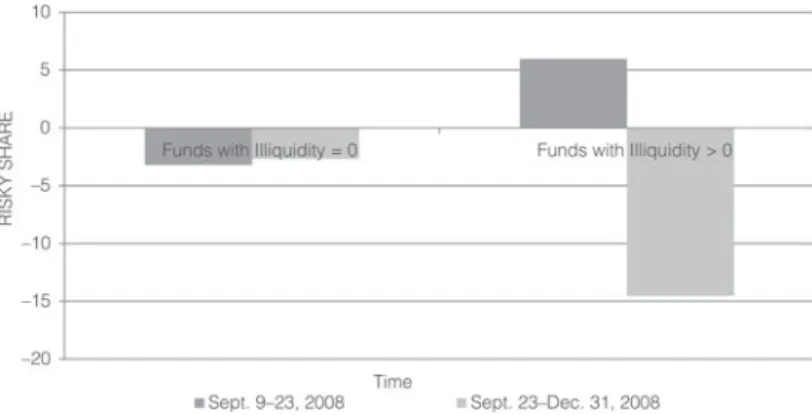
Figure 3 illustrates perhaps the simplest way to digest the combined results of our short- and long-run analyses. Among the prime funds not hit hard by out-flows (those with ILLIQUIDITY= 0), risky assets fell by 3.2% on average dur-ing the run (from Sept. 9 to Sept. 23) and fell an additional 2.7% of net assets by the end of the year. In contrast, among prime funds hit hard by outflows (those with ILLIQUIDITY> 0), risky assets rose by 6.0% during the run (because they were forced to sell nonmaturing, safe assets), but then fell by 14.5% of assets

, on

25 Aug 2017 at 13:17:02