PARALLEL MACHINE SCHEDULING
SUBJECT TO MACHINE AVAILABILITY
CONSTRAINTS
A THESIS
SUBMITTED TO THE DEPARTMENT OF INDUSTRIAL ENGINEERING
AND THE INSTITUTE OF ENGINEERING AND SCIENCE OF BILKENT UNIVERSITY
IN PARTIAL FULFILLMENT OF THE REQUIREMENTS FOR THE DEGREE OF
MASTER OF SCIENCE
By Kaya Sevindik
I certify that I have read this thesis and that in my opinion it is fully adequate, in scope and in quality, as a thesis for the degree of Master of
Science.
Asst. Prof. Mehmet Rüştü Taner (Advisor)
I certify that I have read this thesis and that in my opinion it is fully adequate, in scope and in quality, as a thesis for the degree of Master of
Science.
Prof. M. Selim Aktürk
I certify that I have read this thesis and that in my opinion it is fully adequate, in scope and in quality, as a thesis for the degree of Master of
Science.
Asst. Prof. Yavuz Günalay
Approved for the Institute of Engineering and Sciences:
Prof. Mehmet Baray
ABSTRACT
PARALLEL MACHINE SCHEDULING
SUBJECT TO MACHINE AVAILABILITY
CONSTRAINTS
Kaya Sevindik
M.S. in Industrial Engineering
Supervisor: Asst. Prof. Mehmet Rüştü Taner January 2006
Within a planning horizon, machines may become unavailable due to unexpected breakdowns or pre-scheduled activities. A realistic approach in constructing the production schedule should explicitly take into account such periods of unavailability. This study addresses the parallel machine-scheduling problem subject to availability constraints on each machine. The objectives of minimizing the total completion time and minimizing the maximum completion time are studied. The problems with both objectives are known to be NP-hard. We develop an exact branch-and-bound procedure and propose three heuristic algorithms for the total completion time problem. Similarly, we propose exact and approximation algorithms also for the maximum completion time problem. All proposed algorithms are tested through extensive computational experimentation, and several insights are provided based on computational results.
Keywords: Scheduling, Parallel Machines, Total Completion Time,
ÖZET
MAKİNA KULLANIM KISITLARI ALTINDA
PARALEL MAKİNA ÇİZELGELEME
PROBLEMİ
Kaya Sevindik
Endüstri Mühendisliği, Yüksek Lisans
Tez Yöneticisi: Yard. Doç. Dr. Mehmet Rüştü Taner Ocak, 2006
Bir planlama çevreninde makinalar beklenmeyen bozulmalar veya daha önceden çizelgelenmiş aktiviteler nedeniyle kullanılabilirliklerini kaybedebilirler. Üretim çizelgelemesini gerçekçi bir yaklaşımla oluştururken bu tür kullanılamama periyotlarını hesaba katmak gerekir. Bu çalışma her makinada kullanım kısıtı altında paralel makina çizelgeleme problemi üzerinedir. Toplam bitirme zamanını enazlama ve en büyük bitirme zamanını enazlama hedef fonksiyonları çalışılmıştır. Her iki problemde NP-zor olarak bilinir. Toplam bitirme zamanını enazlama problemi için kesin bir dallandır-ve-sınırla prosedürü geliştirilmiş, ve üç farklı sezgisel yaklaşım algoritması önerilmiştir. Ayrıca en büyük bitirme zamanını enazlama problemi için bir kesin ve bir sezgisel yaklaşım algoritması önerilmiştir. Önerilen bütün algoritmalar kapsamlı ölçümleme deneylerinde test edilmiş ve ölçümleme sonuçlarından muhtelif bulgular sağlanmıştır.
Anahtar Sözcükler: Çizelgeleme, Paralel Makinalar, Toplam Bitirme
Acknowledgement
I would like to express my sincere gratitude to Asst. Prof. Dr. Mehmet Rüştü Taner for him supervision and encouragement in this thesis. His vision, guidance and leadership were the driving force behind the work. His endless patience and understanding let this thesis come to an end.
I am indebted to Prof. Dr. M. Selim Aktürk and Asst. Prof. Dr. Yavuz Günalay for accepting to read and review this thesis and also for their valuable comments and suggestions.
I would like to extend my deepest gratitude and thanks to my mom, dad, sister and my whole family for their continuous morale support, endless love and understanding.
And my sincere thanks to my officemates in EA332 and fellows from Industrial Engineering Department with whom I have shared my time during my graduate study for their patience and help.
Contents
1. Introduction 1
2. Literature Review 3
2.1. Parallel Machine Scheduling... 3
2.2. Scheduling with Availability Constraints... 5
2.3. Summary... 10
3. Total Completion Time Problem 11 3.1. Problem Definition... 11
3.2. Solution Characteristics... 14
3.3. Lower Bound... 18
3.4. Solution Methods... 19
3.4.1. Branch-and-Bound Algorithm... 19
3.4.1.1. Lower Bound for a Partial Schedule. 20 3.4.1.2. Node Generation Process... 21
3.4.2. Heuristic Algorithms... 24
3.4.2.1. Constructive Heuristic Algorithm.... 24
3.4.2.2. Neighborhood Search Algorithm... 30
3.4.2.3. Simulated Annealing Application.... 37
3.5. Computational Experimentation... 39
3.5.1. Experimental Design... 39
4. Maximum Completion Time Problem 46
4.1. Problem Definition... 46
4.2. Solution Procedure... 49
4.2.1. Cutting Plane Scheme... 49
4.2.2. Exact Solution... 52 4.2.2.1. Lower Bound... 52 4.2.2.2. Exact Algorithm... 53 4.2.3. Heuristic Approach... 61 4.2.3.1. Knapsack Algorithm... 62 4.2.3.2. Heuristic Algorithm... 64 4.3. Computational Study... 67 5. Conclusion 72 References 74
List of Figures
3-1 Schematic representation of the problem 12 3-2 Representation of the partial schedule 21
3-3 Node generation process 22
3-4 Back-processing 23
3-5 Partial graph 23
3-6 Worst case solution obtained from “Greedy” 25
3-7 Worst case example of “Greedy” 28
3-8 Representation of NS algorithm 33
3-9 Graphical illustration of initial schedule 34 3-10 Schedule obtained after first move 35 3-11 Schedule obtained after second move 36 3-12 Heuristic performance against the optimum in 30-job
problems 42
3-13 Heuristic performance against the optimum in 50-job
problems 44
3-14 Heuristic performance against the optimum in 70-job
problems 45
4-1 Schematic view of exact algorithm 55 4-2 Schematic representation of the partial schedule 56 4-3 Availability intervals preceding unavailability periods 61
List of Tables
3-1 Processing times of jobs 34
3-2 Initial solution 34
3-3 Schedule obtained after the first move 35 3-4 Schedule obtained after the second move 36 3-5 Experimental scheme of unavailability periods 40
3-6 Branch-and-bound results 40
3-7 Results of heuristic algorithms for 30 jobs 42 3-8 Results of heuristic algorithms for 50 jobs 43 3-9 Results of heuristic algorithms for 70 jobs 44 4-1 Exact algorithm results for one unavailability period 69 4-2 Exact and heuristic algorithm results for cases
pi ~ U(1,70) 70
4-3 Exact and heuristic algorithm results for cases
Chapter 1
INTRODUCTION
Scheduling literature commonly assumes that machines are continuously available throughout the entire planning horizon. This assumption may not hold in many cases where unexpected breakdowns occur or when some activities are pre-scheduled on machines. Models and findings in the general scheduling literature may become inadequate to find optimum solutions for many cases with machine availability constraints. Although scheduling with availability constraints has gained some popularity during the last decade, there are still gaps in the relevant literature with respect to various machine arrangements and objective functions.
This study considers parallel machine scheduling problem with availability constraints on each machine with the objectives of minimizing total completion time (
∑
Cj ), and minimizing maximum completion time (makespan, Cmax). The problems with both objectivesare known to be NP-hard [18], [35]. There is exactly one unavailability period on each machine. Durations of unavailability periods are deterministic and can be different on different machines. Unavailability periods are non-simultaneous for total completion time problem, however they can be simultaneous in makespan problem.
Chapter 2 gives a short review of the literature on parallel machine scheduling problems with the objectives of minimizing Cmax and
minimizing and the literature on machine scheduling with availability constraints. Chapter 3 defines the problem of minimizing
,
j C
j C
∑
with availability constraints, proposes exact and heuristic solution methods for this problem, and presents computational results with the proposed methods. Similarly, Chapter 4 focuses on the problem of minimizing Cmax with availability constraints, develops exact andheuristic solution methods for this problem, and presents computational results. Finally, Chapter 5 concludes the thesis with a summary of the major findings, and gives some directions for future research.
Chapter 2
LITERATURE REVIEW
This section provides a literature review of parallel machine scheduling with objectives of minimizing Cmax and
∑
Ci, and machine schedulingwith availability constraints.
2.1. PARALLEL MACHINE SCHEDULING
Elaborate reviews of the literature on parallel machine scheduling are provided in [44] and [10]. The problem with the objective of minimizing the total completion time (∑
Ci) can be solved in polynomial time [13]. It is well known that the problem of minimizing makespan (Cmax) onparallel identical machines is NP-hard even with two machines [18], [19]. Dell’Amico and Martello [16] introduce lower bounds, heuristic algorithms and a branch-and-bound algorithm, and Ho and Wong [24] implement a lexicographical search procedure for this problem. The most recent exact procedure in the literature is the branch-and-cut algorithm developed by Mokotoff [46]. Dell’Amico and Martello [17] show that their original algorithm proposed in [16] outperforms this recent algorithm proposed by Mokotoff in [46] by some orders of magnitude.
The unrelated parallel machine problem with the objective of minimizing
Cmax is also widely studied. Exact and approximate algorithms for this
problem are presented in Van de Velde [53], and Martello et al. [42]. The most recent exact procedure is the cutting plane scheme developed by Mokotoff and Chretienne [45]. Ghirardi and Potts [21] propose a
recovering beam search algorithm in a recent study. Other examples of heuristic attempts include Mokotoff and Chretienne [45], Martello et al. [42], Horowitz and Sahni [25], Ibarra and Kim [26], De and Morton [15], Davis and Jaffe [14], Potts [48], Lenstra et al. [37], and Hariri and Potts [23]. Chang and Jiang [9] address an extension of the problem that incorporates arbitrary precedence constraints and develop a state-space-search procedure for its solution.
Salem et al. [50] consider an extension of the problem with machine eligibility restrictions in which a subset of the jobs can be processed only on certain machines. They propose a branch-and-bound algorithm that exploits a customized lower bound. Their algorithm is capable of efficiently solving instances with up to 8 machines and 40 jobs.
The problem of preemptive task scheduling on parallel identical machines with the objective of minimizing the Cmax can be solved in
polynomial time in most cases even if there are precedence constraints. Muntz and Coffman [47] propose an algorithm for the case in which there are tree-like precedence constraints on parallel machines.
Bruno et al [8] show that the problem of scheduling jobs on parallel identical machines with the objective of minimizing the total weighted completion time is NP-hard even with two machines. Azizoglu and Kirca [4] consider both the identical and the uniform machine cases of the multi-machine problem, establish optimality characteristics, develop a lower bound, and construct a branch-and-bound algorithm.
2.2. SCHEDULING WITH AVAILABILITY
CONSTRAINTS
Schmidt [52] and Sanlaville and Schmidt [51] provide an excellent review of scheduling with machine unavailability. These reviews present single, parallel, and flow shop models with total completion time, Cmax,
and due date related objectives.
Research on single machine problems under machine availability constraints is very limited. Lee and Liman [34] show that the problem of minimizing on a single machine without preemption is NP-hard. Sadfi et al. [49] study the single machine scheduling problem with a given unavailability period and deterministic processing times. They consider the total completion time objective and propose an approximation algorithm with a worst-case error bound of 20/17. Akturk
et al. [2] study single machine problem with multiple unavailability
periods by minimizing total completion time. They provide a number of heuristic methods and discuss the performances of these heuristics through computational experiments. Akturk et al. [3] also consider the SPT (Shortest Processing Time) list scheduling for the same problem and they provide worst case bounds under different conditions. Lee and Leon [33] consider the single machine scheduling problem with a rate-modifying activity in which the starting time of the rate rate-modifying activity is a decision variable. They develop polynomial time algorithms for the C
i C
∑
max and total completion time objectives, and a
pseudo-polynomial algorithm for a special case of the total weighted completion time problem. Lee and Leon also show in this paper that the problem of minimizing maximum lateness is NP-hard, and they provide a
pseudo-polynomial algorithm. Graves and Lee [22] study a single machine scheduling problem with maintenance windows and semi-resumable job processing with the starting time of the maintenance a decision variable. They show that the problem of minimizing the total weighted completion time is NP-hard, while the SPT and EDD (Earliest Due Date) ordering give optimal schedules for the total completion time and Lmax objectives,
respectively. Liao and Chen [39] study the single machine problem with multiple periods of unavailability with the objective of minimizing maximum tardiness. They develop both an exact branch-and-bound procedure and a heuristic algorithm.
Parallel machine problems with the objectives of minimizing Cmax, and Lmax tend to be polynomially solvable when preemption is allowed.
Although polynomial time algorithms can be found for some special cases, most non-preemptive problems are known to be NP-hard.
Lee [29] studies parallel identical machine scheduling problem with initial availability constraints. He studies the objective of minimizing
Cmax, and provides a polynomial time approximation algorithm with a
worst-case error bound of 4/3.
Liao et al. [40] study the objective of minimizing Cmax on two parallel
machines with an availability constraint during a given interval on only one machine. They classify the problem into four cases, and use versions of a lexicographical search algorithm originally proposed by Ho and Wong [24] to device an exact method for each case.
Gharbi and Haouari [20] consider the parallel identical machine problem with non-decreasing and non-simultaneous machine availability times,
release dates, and delivery times and the objective of minimizing Cmax.
They develop new lower and upper bounds based on max-flow computations, and propose a branch-and-bound algorithm using these bounds. This algorithm is able to solve instances with up to 700 jobs and 20 machines.
Leung and Pinedo [38] study a preemptive problem with identical parallel machines, and deterministic unavailability periods. They consider the total completion time, Cmax and maximum lateness
objectives. For the total completion time objective, they show in what conditions the optimum solution can be obtained via list scheduling. For the Cmax objective, they consider problems with precedence constraints
and fixed processing times. They determine conditions on precedence constraints and on unavailability periods to find a polynomial time algorithm. They also give a polynomial time algorithm that gives optimum solutions for the Lmax and Cmax objectives without any
precedence constraints.
Blazewicz et al. [5] also consider the preemptive problem case when machines are available for processing for certain time intervals with precedence constraints. They show that the P, staircase/pmtn, intree/Cmax
problem is NP-hard in the strong sense. They propose a polynomial time, linear programming based procedure to solve the case with chain-like precedence constraints and a staircase pattern of machine availability. They also study uniform and unrelated parallel machine problems with arbitrary patterns of unavailability with the Cmax and Lmax objectives.
They propose a network flow approach for the uniform, and a linear programming approach for the unrelated machine problem.
Lee and Liman [34] study the two parallel machine scheduling problem with an unavailability period on one machine with the objective of minimizing the total completion time. They show that the problem is NP-hard, and propose a pseudo-polynomial, online algorithm as well as a constructive heuristic with a worst-case error bound of 3/2. Kaspi and Montreuil [27], and Liman [41] study the same problem, and show that in the special case involving only initial availability constraints, SPT ordering gives the optimum solution.
Lee and Chen [32] study the problem of scheduling jobs and maintenance activities on parallel machines with the objective of minimizing the total weighted completion time. As in [22], the starting times of the maintenance activities are taken as decision variables. The authors consider the two cases of overlapping and non-simultaneous periods of unavailability. They show that the problem is NP-hard in both cases. They propose a branch-and-bound method based on column generation techniques to solve medium sized problems within a reasonable computational time.
Lee and Lin [36] study a single-machine scheduling problem with stochastic breakdowns, and a rate modifying maintenance/repair activity. They consider the objectives of expected Cmax, total expected completion
time, expected maximum lateness, and maximum expected lateness. A machine becomes unavailable due to a maintenance activity triggered by the decision maker who wishes to increase its speed or repair activity required due to a fatal breakdown. The machine assumes its normal speed after the repair/maintenance activity.
All studies on the flowshop problems with machine unavailability focus on the Cmax objective. Lee [30] studies a two-machine flowshop
scheduling problem of minimizing Cmax with an availability constraint.
He considers a fully deterministic environment. He shows that the problem is NP-hard and develops a pseudo-polynomial algorithm to solve the problem optimally. In addition, he develops two heuristic algorithms each having a complexity of O(n log n). The worst-case error bound of his first algorithm, which is proposed for problems with an availability constraint on machine 1, is 3/2, and that of his second algorithm for problems with an availability constraint on machine 2 is 4/3. Cheng and Wang [11] address the same problem in [30] and show that the relative worst-case error bound of 3/2 is tight for the heuristic proposed in [30] when there is an availability constraint on machine 1. Also, they propose an improved heuristic algorithm with a relative worst-case error bound of 4/3.
Blazewicz et al. [6] study the same problem with availability constraints on both machines. They analyze several constructive and local search based algorithms in the literature through computational experimentation.
Cheng and Wang [12] study the generalization of the problem studied in [30] in that having an availability constraint imposed on each machine. Availability constraints are consecutive. They identify some characteristics of the problem in the semi-resumable case, and provide a heuristic with a relative worst-case error bound of 5/3 for the non-preemptive case. Breit [7] also studies the non-preemptive version of the problem in [30] with an availability constraint only on machine 2. He proposes a heuristic algorithm with a worst-case error bound of 5/4.
Lee [31] considers the two-machine flowshop problem and an availability constraint on only one machine and on both machines. Job processing is semi-resumable where if a semi-resumable job is interrupted by an unavailability period, the processing can continue with after a certain setup time. He provides a complexity analysis, develops a pseudo-polynomial dynamic programming algorithm, and proposes heuristics supplemented with error bounds.
Aggoune [1] considers m-machine flowshop scheduling problem with availability constraints with the objective of minimizing Cmax. He studies
two cases of the problem. In the first case, starting times of unavailability periods are fixed, while in the second case starting times are in a time interval. He proposes a genetic algorithm and a tabu search procedure.
2.3. SUMMARY
Total completion time problem on the parallel machines with continuous availability is easy to solve, however, makespan problem turns out to be
NP-hard. Extensive research is conducted on makespan problem on
parallel machines, which includes identical, uniform and unrelated parallel machines. With availability constraints, single and parallel machine scheduling problems are NP-hard for both total completion time and makespan objectives. Although problems with availability constraints have become very popular for the last decade, the relevant literature is still very limited. For both objectives minimizing
∑
and makespan, this study fills the gap in literature of scheduling problems with availability constraints on each of parallel machines.i C
Chapter 3
TOTAL COMPLETION TIME
PROBLEM
This section defines the problem of minimizing
∑
Cj on parallel identical machines with availability constraints, develops exact and heuristic solution methods for this problem, and presents computational results with the proposed methods.3.1. PROBLEM DEFINITION
All jobs are released simultaneously. Processing times are known and deterministic. Each job is to be processed exactly on one of the parallel identical machines. Job processing is non-preemptive. There is exactly one unavailability period on each machine for which the starting time and duration are given. Periods of unavailability on different machines do not overlap. That is, at most one machine may become unavailable at any time instance. This assumption is required since the lower bound to be defined in section 3.3 would not be valid without it.
Since this particular problem is a more general version of the one that is proved to be NP-hard by the Lee and Liman [35], it is also NP-hard.
MATHEMATICAL FORMULATION
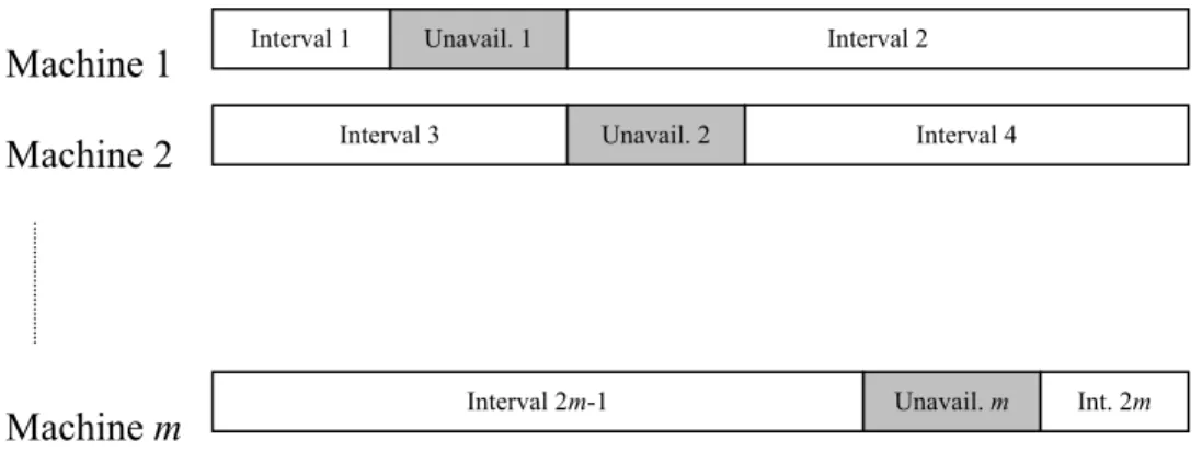
The schematic representation of the problem is as follows. Available times of machines for processing before and after the unavailability periods will be denoted as “availability intervals” or only “intervals”. Every machine has two “intervals” for processing jobs. There are 2m intervals for processing in the system in cumulative.
Interval 2 Interval 1 Unavail. 1 Machine 1 Unavail. 2 Interval 4 Interval 3 Machine 2 Int. 2m Interval 2m-1 Unavail. m Machine m
Figure 3-1 Schematic representation of problem
Define ai as the starting time of the interval i, that is ai = 0 for intervals i
= 1, 3,…, 2m-1; but ai equals to the summation of starting time and
duration of the unavailability period on the corresponding machine for intervals i = 2, 4,…, 2m .
The notation is as follows. Indices:
h : Machine index, h= 1,2,…,m
j, k, l, g : Job index, j, k, l, g = 1,2,…,n
i: Interval index, i = 1,2,…,2m
Parameters:
sh: Starting unavailability period on machine h
pk: Processing time of job k
Sets:
Pk: Set of jobs preceding job k in the same interval; Sk: Set of jobs succeeding job k in the same interval;
Decision variables:
xik: 1 if job is processed in interval
0 otherwise k i = bjk
1 if jobs and are processed in the same interval
0 otherwise
j k
=
rk: Starting time of the processing of job k;
Assume without loss that jobs are indexed in SPT order, that is,
1 2 ... n
p ≤ p ≤ ≤ p . Then, the problem can be formulated as follows.
min 2
(
)
1 1 m n ik i k k i k x a r p = = + +∑∑
Subject to 2 1 1 m ik i x = =∑
for ∀k (3.1) 1 jk ij ikb ≥x +x − for i=1,...,2m and ∀j k, s.t j<k (3.2)
1 1 k k jk j r − b = ≥
∑
pj for ∀k (3.3) 2 1, 1 n h k k h k x − p s = ≤∑
for h=1, 2,…, m (3.4)rk ∈ N for ∀k
Constraint set (3.1) ensures that all jobs are assigned to exactly one of the intervals. Constraint set (3.2) determines which jobs are processed in the same interval. Constraint set (3.3) indicates that the starting time of a job cannot be any smaller than the sum of the processing times of the preceding jobs within the same interval, and a job is preceded by the jobs with smaller processing times. Finally, constraint set (3.4) ensures that all jobs scheduled to be processed before unavailability can be completed so as to allow for the corresponding unavailability period to start on time.
3.2. SOLUTION CHARACTERISTICS
It is shown that SPT ordering minimizes the total completion time on continuously available, parallel identical machines. However, SPT ordering is not the only solution for this case. Consider two-parallel machine case, there are 2n/ 2 ( x
is the greatest integer strictly smaller
than x) optimal solutions for the problem where n is the number of jobs to be completed. As stated before, jobs are indexed in SPT order. Then the completion time of job j in the optimal schedule is:
j
j k
k P
C p
∈
=
∑
+ p . It can be seen that every job takes place in the jcalculation of completion time of the jobs succeeding it. If we do some algebraic operations the total completion time turns out to be
1 ( 1) n j j j S p = +
∑
where Sj is the number of jobs in Sj. It can be seen thatinterchanging the place of a job with the place of another job with same number of successors (interchange place of jobs j and k s.t. |Sj| = |Sk|)
does not violate optimality. Since the number of jobs holding this condition is in two-parallel machine problem, there are 2 optimal solutions. Therefore, SPT ordering is a sufficient but not a necessary condition for optimality in the case of continuous machine availability. For the same case, a general necessary and sufficient condition can be summarized as follows.
/ 2 n n/ 2 l k P C = + k j l l P l∈ = +
∑
Sj pjLemma 3.1: Let k and j be two jobs assigned to different machines with processing times pk and pj such that pk < pj. Then in the optimal solution
k j
S ≥ S .
Proof: By contradiction. Suppose jobs k and j with pk < pj are scheduled
in the optimal solution such that Sk < Sj . Then the objective value is
1 k k j n j g l l j g l l S l P l S C C C C C = ∈ ∈ ∈ ∈ + + + +
∑
∑
∑
∑
∑
Clif we exchange the places of jobs k and j, completion times of jobs that precede these jobs remain the same, and completion times of jobs k and j become
Ck = rj + pkand Cj = rk +pj, respectively.
Thus, the summation of Ck and Cj does not change. However starting
times of jobs succeeding job k in the original schedule increase by pj– pk
and that of jobs succeeding job j in the original schedule decrease by pj– pk. As a result, the new objective value after the exchange is:
* 1 ( ) ( ) k j n g k j l l k j k g l P l S l S C C C C C C C S p p p = ∈ ∈ ∈ + + + + + − − −
∑
∑
∑
∑
k(
)
* 1 1 ( ) n n g l j k j g l C C S S p = = = − − −∑
∑
pkWe know that Sk < Sj and pk < pj. Hence, the
∑
Cg in the new schedule is strictly smaller than that in the original schedule. Therefore, there cannot be an optimal schedule withk
S < Sj and pk < pj.
Corollary 3.1: For the continuous available machines case, jobs assigned to the same machine must be processed in SPT order in the optimal schedule.
Optimality Conditions
Because jobs are non-preemptive and starting time and duration of each interval is fixed, jobs assigned to different intervals may not have easily identifiable precedence relations. Intervals before unavailability periods have a processing capacity; hence certain jobs cannot be processed together in these intervals. This makes it very difficult to find precedence relations valid for every problem instance.
Observations on the parallel machine problem with continuously available machines lead to the following optimality properties.
Corollary 3.2: Jobs must be sequenced in SPT order within each interval.
Proof: The sub-problem within each interval can be thought of as a single machine problem, and it is well known that SPT ordering minimizes the flow time, [3].
Define Ii as the idle time left in interval i in the optimal schedule. Since
the period of unavailability, respective idle times in intervals 2, 4,…,2m are always zero. Idle times for intervals before the unavailability period equal to the difference between the initial available processing time of the corresponding interval and cumulative processing time of jobs assigned to that interval.
i i i j As j I Av p ∈ = −
∑
.Where Avi = s(i+1)/2 that is starting time of period of unavailability on the
corresponding machine, and Asi is the set of jobs assigned to intervals i
where (i = 1,3,…,2m-1).
Lemma 3.2: Let g, j, k, and l be four jobs with processing times pg < pj < pk < pl respectively. Suppose job j is assigned to interval x, and job k is
assigned to interval y in the optimal solution. Let g be the last job assigned to interval y with a smaller processing time than j, and let l be the first job assigned to interval x with larger processing time than k. Then at least one of the following two conditions must hold for optimality:
i) The places of job j and job k cannot be exchanged due to availability
constraint, that is: x j k
I + p < p
ii) The total gain obtained from the exchange of the places of job j and
job k is not positive that is:
(
1)
(
1)
j j g j k k l k
S ×p − S − ×p + S ×p − S + ×p ≤ 0
Proof: By contradiction. Suppose neither condition holds in the optimal solution. That is, there exists an optimal schedule S such that
ii)
(
Sg − ×1)
pj − Sj ×pj+(
Sl + ×1)
pk− Sk ×pk < 0 kThat Ix+ pj ≥ p implies interchanging jobs j and k leads to a new feasible solution. If we exclude job j from interval x and job k from interval y the gain is
j j k
S ×p + S ×pk
And if we assign job j to interval y and job k to interval x the increase in the objective value is
(
Sg − ×1)
pj+(
Sl + ×1)
p then total gain is k(
)
(
Sj − Sg −1)
pj +(
Sk −(
Sl +1)
)
pkOpening of the term above is the same as the term in condition (ii), multiplied by (-1). Hence, adding these gives a positive gain in the objective value. Hence, any schedule that satisfies both of the two conditions above cannot be an optimal solution.
3.3. LOWER BOUND
Leung and Pinedo [38] show that Shortest Remaining Processing Time (SRPT) order gives an optimum solution to the parallel machine problem subject to machine unavailability and preemptive processing times.
Since all solutions for non-preemptive case is also feasible solutions for preemptive case, the optimum solution of the preemptive case dominates all solutions for the non-preemptive case. Hence, the preemptive solution constitutes a lower bound for our problem.
This lower bound is expected to perform better in those problems in which the periods of unavailability on all machines occur both close to
either the beginning or the end of the planning horizon. Keeping in mind that the lower bound sets the idle time immediately preceding the interval of unavailability on each machine equal to zero, this insight can be explained by the following two observations on the optimum solution.
Observation 1: The length of the idle time tends to be larger as the starting time of the unavailability gets larger.
Observation 2: The number of succeeding jobs amplifies the impact of the length of the idle time on the objective, when the starting time of unavailability gets smaller.
The total impact on the objective tends to assume its maximum level when the starting time of unavailability lies in the medium term, and both factors are in play. Hence, the expected poorer performance in the lower bound for such cases.
3.4. SOLUTION METHODS
We identify some problem characteristics in Section 3.2. We use these characteristics to develop exact and heuristic algorithms for the problem. In this section we present our solution methods to find exact and approximate solutions for the problem and we discuss our exact and approximate algorithms in detail.
3.4.1. BRANCH-AND-BOUND ALGORITHM
We propose a branch–and–bound algorithm to solve small- and medium-sized problems optimally. As mentioned before, given the job
assignments to the intervals SPT ordering within each interval gives an optimal solution. Hence, the key decision is how to assign the jobs to the intervals.
3.4.1.1. Lower Bound for a Partial Schedule
A modification of the overall lower bound obtained from the solution to the preemptive problem gives a lower bound for each particular schedule corresponding to the nodes of the branch-and-bound tree. Level 0 in the branch-and-bound tree defines that no job is assigned any of the intervals. In the level 1, decision of assigning the job with SPT is done, and for the next levels this continues with remaining jobs in SPT order. Fixing the assignment of job k (level k) to the corresponding interval and assigning the remaining jobs by SRPT, calculate lower bound for a node at level k. While calculating the lower bund for a node at level k, the key point is jobs fixed to intervals should be the first k jobs in SPT order of all jobs.
Obviously, processing the jobs not included in each particular schedule in
SRPT order gives a lower bound for that particular schedule. This lower
bound can be strengthened through a modification based on the following observations.
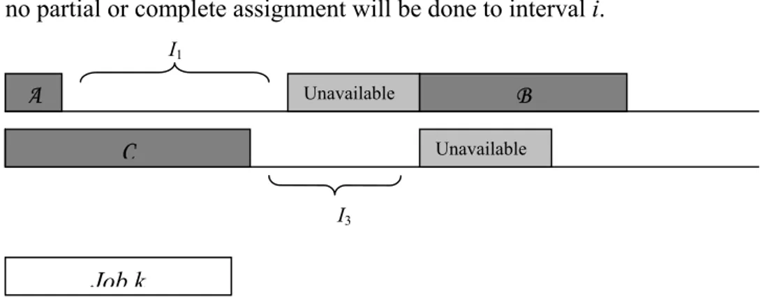
Fact 1(Look Ahead Factor): Let S be a given partial schedule and, let Jk
be the next job to be assigned, that is, first k – 1 jobs are fixed and job k is the job with the SRPT. This scheme belongs to (k – 1)th level of the branch-and-bound tree. If Jk cannot be assigned to interval i (i
– 1}) for the partial schedule P is smaller than pk, for this and next levels,
no partial or complete assignment will be done to interval i.
I1 B Unavailable C A Unavailable I3 Job k
Figure 3-2 Representation of the partial schedule
Consider the two-machine case above. Suppose that A, B and C are set of jobs assigned respectively intervals 1, 2, and 3 in partial schedule P. Suppose that I1 is greater than or equal to pk whereas the I3 is smaller
than pk. According to fact, there will be no assignments to interval 3 until
the branch-and-bound algorithm back-processes to (k – 1)st level.
3.4.1.2. Node Generation Process
Let n be the number of jobs and assume without loss jobs are indexed in
SPT order. Number of jobs in the partial schedule designates the level in
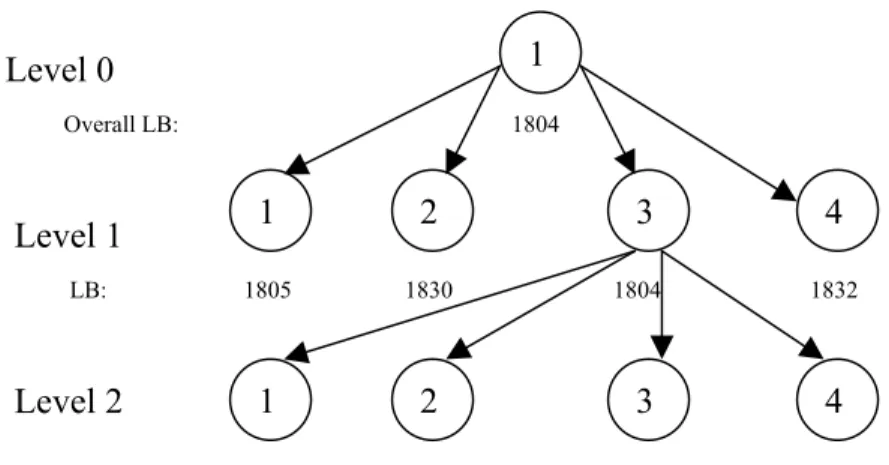
the branch-and-bound tree, and the nodes within each level correspond to the intervals to which the next job can be assigned. Since the jobs are indexed in SPT order, level 1 corresponds to job 1, level 2 corresponds to job 2 and so on. At each level a new set of nodes are generated by assigning the next job to each one of the 2m possible intervals. Then the lower bound is taken as the best promising node. This best promising node is selected as the parent node for the next level, and the process repeats itself until all jobs are scheduled. Hence, a job is assigned to an interval; the algorithm passes on the next job with the smallest processing time.
Level 0 Overall LB: 1804 Level 1 LB: 1805 1830 1804 1832 4 2 3 1 4 1 3 2 1 Level 2
Figure 3-3 Node generation process
Figure 3-3 depicts levels 0-2 for a branch-and-bound tree for a hypothetic scenario of a two-machine problem example, the overall lower bound for the problem is 1804, that is also the lower bound for node 1 at level 0. At level 1, the first job is assigned to each of the four intervals, and the corresponding lower bounds are calculated. At level 2, four new nodes are generated from the node gave the smallest lower bound in level 1.
When it is not possible to generate new nodes from the current node, back-processing runs. For instance, when the last job is inserted to an interval, there remains no jobs to be inserted to generate nodes or when all possible nodes that can be generated from a node do not give a lower bound that is better than the current feasible solution.
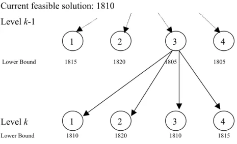
In the back- processing current node’s lower bound is updated as the best of the lower bounds of its child nodes, and process returns to the previous node (level).
Current feasible solution: 1810 Level k-1 Lower Bound 1815 1820 1805 1805 4 3 2 4 3 2 1 1 Level k Lower Bound 1810 1820 1810 1815 Figure 3-4 Back-processing
Consider a two-machine problem; at level k we have a feasible solution with a total completion time (
∑
Cj) value of 1810. As it can be seen in the Figure 3-3, no other node at the same level has a potential to lead to a better solution. Thus, the algorithm proceeds at level k – 1, equal to lower bounds of its child nodes as 1810, and deletes all of the lower bounds of nodes in level k.The resulting partial graph is shown in Figure 3-5
1 2 3 4
Level k-1
Lower Bound 1815 1820 1810 1805 Figure 3-5 Partial graph
Since only node 4 in level k – 1 has a corresponding lower bound that is smaller than that of the best incumbent solution, the process continues by generating 4 new branches, emanating from this node. The algorithm stops with the optimal solution, when all updated lower bounds of the nodes in level 1 is greater than or equal to the best incumbent solution so far found.
3.4.2. HEURISTIC ALGORITHMS
Since our problem is NP-hard exploration of heuristic approaches is justified. Consequently, in this section, we exploit the previously identified optimality properties to propose a constructive heuristic algorithm, a neighborhood search mechanism, and a simulated annealing application.
3.4.2.1. Constructive Heuristic Algorithm
This algorithm, called Greedy Assignment (Greedy) is based on greedy assignments of jobs to the intervals by using the “lower bound” of a partial schedule defined in Branch-and-Bound section. The algorithm starts with the first job (the job with SPT), assigns this job to the interval, which gives the minimum lower bound, and continues with next jobs in the order of SPT. The solution obtained from Greedy is used as the initial feasible solution in the branch-and-bound algorithm.
Although the algorithm assigns jobs with respect to lower bounds, resulting schedule has some intelligence due to the look ahead factor in the lower bound calculation. This factor allows the algorithm not to assign jobs to the intervals before the unavailability periods resulting large idle times in these intervals.
Worst Case Error Bound of Greedy
Let POPT be the optimal solution for the preemptive case of the problem and GSOL and NOPT are the heuristic and optimum solutions for the non-preemptive case of the problem. We know that SRPT ordering of preemptive case gives a lower bound for the non-preemptive case that is,
POPT ≤ NOPT for all problem instances.
Define minsum(x)(y1,…, yz) that equals to summation of first x smallest
values of the set (y1,…, yz). For instance, minsum(2)(2, 3, 4) = 2 + 3.
Similarly, define maxsum(x)( y1,…, yz) that equals to summation of first x
largest values of the set (y1,…, yz). For instance maxsum(2)(2, 3, 4) = 3 +
4. Also define xy that equals to “x – x y/ ×x”. For instance, 42 = 2 and
32 = 1. Let z be the smallest integer that is greater than or equal to z.
Theorem 3.1: When the periods of unavailability on different machines are of equal length, the worst case error bound of the Greedy algorithm is 2.
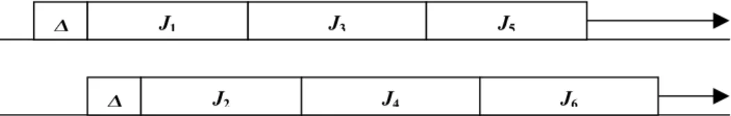
Proof: The greatest deviation between GSOL and POPT is obtained when there is no job assignment in intervals before unavailability periods. Figure 3-6 depicts the particular 2-machine case, where ∆ is the length of a period of unavailability.
J6 J4 J2 ∆ J5 J3 J1 ∆
Assume without loss of generality s1 < s2 <…<sm. For m-machine case,
greedy gives a solution displaying this characteristic if and only if p1 ≥ sm where sm is the starting time of unavailability period on machine m.
Also we know that sm ≥ (m–1)∆, as the unavailability periods do not
overlap. For the worst case defined above, “Greedy” finds a solution (GSOL) of:
(
)
(
)
(
)
(
)
(
)
(
)
1 1 1 2 1 1 2 1 2 ... 1 ... 2 ... ... ... ... 1 ... (3.5) m m m m m m n n n m n m n m n m n n m n n p p p p m m n p p p p m n s s s s s s m + + + + + − + + + + − + + + − + + + + + + + + ∆ + + ∆ + + + ∆ + − + ∆ + + ∆ + + + ∆ In the other hand, SRPT finds a solution (POPT) for preemptive case:
(
)
(
)
(
)
(
)
(
)
(
)
(
)
(
)
(
)
(
)
(
)
1 1 1 1 2 3 1 ( ) 1 1 2 3 1 ( ) 1 ... 1 min , max , , , ,..., , 1 minsum 1 min , max , , , ,..., , 2 maxsum 1 min , m m m m m m m m n m m m m m m n m m m p p p s m s p s p p p p n m p s m s p s p p p p n m p s m s p − − − − + + + − + − ∆ + + ∆ + + ∆ − + − + − ∆ + + ∆ + ∆ − − + − ∆ + + ∆ (
)
(
)
(
)
1 1 2 1 1 ... 2 ... ... ... (3.6) m m m m m n m n m n n m n n n p p p p m m p p + + + + + − + + − + + + − + + + + + + Since (m-1)∆ ≤ sm, for s1 < s2 <…< sm < p1 ≤ p2 ≤….≤ pn,The deviation between GSOL and POPT is maximized when ∆ → 0, s1
→ p1, pn → p1. In these limits the equations (3.5) and (3.6) tend to
1 1 1 1 1 1 2 ... 1 (3.5) becomes (3.5') and m m n n n n p m p m p m p n p m m m n m p m + − + − + + × + − 1+ 1 1 1 1 1 1 1 1 ( ) 2 1 2 3 ... (3.6) becomes (3.6'). m m m n n n mp n p m n p n p m m m n n m p m p mp m m + − + − − + − − + − + + +
After reordering the terms in both equations and dividing (3.5’) to (3.6’), we obtain (3.5’)/(3.6’): 1 1 1 1 1 1 1 1 1 2 1 2 ... (3.7) 1 2 ... m m m n n n n p n p m p m p m p m m m n n n n p m p m p m p m m m + + − + − + + × + − + − + + ×
After doing some algebraic operations, this ratio becomes 1 1 1 1 2 (3.8) 1 1 2 m m n n n n n m m m m m n n n n m m m + + − + − + −
We can see that this ratio is maximized at n ≤ m, with the value of 2. From the above result, we know that GSOL 2
POPT ≤ for all problem
2
GSOL GSOL
NOPT ≤ POPT ≤ for all problem instances. Therefore, 2 is a worst
case error bound for the Greedy algorithm.
Corollary 3.3: Greedy Algorithm’s worst case error bound of 2 is tight for the 2-machine case.
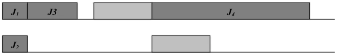
Proof: Now consider the problem instance with 4 jobs with (p1=ε, p2=ε, p3=2ε, p4=s2), 4ε ≤ s1, 7ε≤ s2 and s1 + ∆ = s2.
The Greedy algorithm produces the following solution.
J2
J3
J1 J4
Figure 3-7: Worst case example of “Greedy”
with an objective value 5ε + 2s2. But optimal schedule has an objective
value 7ε + s2. Then the ratio between NOPT and GSOL is:
2 2 5 2 7 s s ε ε + + . 2 0 2 5 2 lim 2 7 s s ε ε ε → + =
+ is the error bound for this instance, and this equals to the worst-case bound of the problem. From this result we can conclude that 2 is the worst-case bound of Greedy algorithm and it is tight.
Theorem 3.2: The Greedy algorithm has a worst-case error bound of 3/2 on the 2-parallel machine problem case, which has only one period of unavailability.
Proof: In the worst case of this type of problem, two criteria must be hold. First, there is no job assignment to the available period before unavailability period, and, second, the number of jobs assigned to the continuously available period is maximized. To hold these criteria, p1 > s
where t is the starting time of unavailability, and 1
1 n j j p s − = ≤ + ∆
∑
.Under these conditions, the solution obtained from Greedy algorithm is
1 ( 1) 2 ... n
n p× + − ×n p + + p (3.9), and solution obtained from SRPT,
1 ( 1) ( 1 2 ) ( 2) 3 ... n p + − ×n p +p − + − ×s n p + + p = 1 ( 1) ( 2 ) ( 2) 3 ... n n p× + − ×n p − + − ×s n p + + p (3.10). If we divide (3.9) to (3.10), we obtain, 1 2 1 2 3 ( 1) ... ( 1) ( ) ( 2) ... n n n p n p p n p n p s n p p × + − × + + × + − × − + − × + + for t < p1 ≤ p2 ≤…≤pn. This ratio is largest
where s→p1,p2→p1,…,pn→p1. Then the ratio becomes
1 1 1 1 ( 1) 2 1 ( 1) ( 1) 2 n n p n n p n p + + − −
and this ratio is maximum at n=2, or n=3, that is
3/2.
We know that 3 2
GSOL
POPT ≤ for all problem instances from above result.
Since NOPT ≥ POPT for all problem instances, 3
2
GSOL GSOL
NOPT ≤ POPT ≤ for all problem instances. Therefore, 3/2 is a worst
Now consider the problem instance with 5 jobs with (p1=ε, p2=ε, p3=ε, p4=t, p5=s + ε), and 3ε ≤ s, the greedy algorithm gives a solution of
= 3s + 10ε while optimal solution is 2s + 10ε. Then the ratio is j C
∑
3 1 2 1 s s 0 0 ε ε ++ . While ε→0, the ratio is 3/2. Hence, 3/2 is a tight upper bound for Greedy.
Corollary 3.4: A more general worst-case error bound for the problems that every machine does not have unavailability periods can be written. Let u be the number of machines that have unavailability periods on it. Then worst-case bound of this algorithm is 1 u
m
+ . This can be proved by the same approach used in Theorem 2.
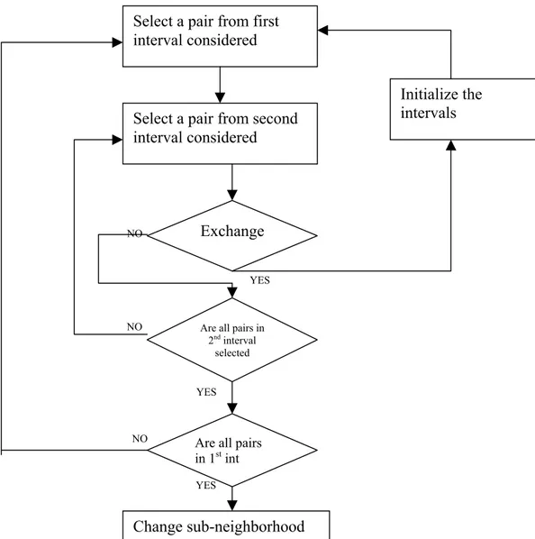
3.4.2.2. Neighborhood Search Algorithm
This algorithm is based on searching for improving solutions from a neighborhood of a given initial feasible solution. Since searching entire solution space is too costly, a small neighborhood of a solution is determined and a search is performed on this neighborhood. An initial feasible solution, a neighborhood structure, and a search structure between the neighborhoods of a feasible solution are defined to construct this neighborhood search mechanism.
Neighborhood Definition
As mentioned before assigning job to intervals are preferred rather than assigning jobs to machines while defining neighborhood structure. Since jobs assigned to each interval of machine availability are to be processed
in SPT order, a feasible assignment of all jobs to these intervals constitutes a solution. Within this framework, the neighborhood of a given feasible solution is defined as the set of new solutions that can be generated through two-, three-, and four-way job exchanges among intervals of machine availability. Two-way job exchanges consist of one to two, three-way job exchanges consist of one to two, and four-way job exchanges consist of two to two job exchanges between 2m intervals defined in section 2.
Whole neighborhood is not searched in only one iteration. To make this search easier and more efficient we divide the whole neighborhood of a feasible solution into sub-neighborhoods. A sub-neighborhood consists of only job exchanges between only fixed 2 intervals. Actually a sub-neighborhood is a sub-neighborhood defined only between two intervals. Local optimum of a sub-neighborhood of a feasible solution is the minimum solution that can be found by making two-, three-, and four-way job exchanges between the corresponding two intervals. In a particular m-machine problem, there are C(m,2) sub-neighborhoods.
For two-machine problem case, in addition to these sub-neighborhoods, 4 dummy sub-neighborhoods are generated for fine-tuning of the algorithm. These 4 sub-neighborhoods search job exchanges between 3 intervals. For a particular two-machine case these intervals are:
[from 2 to 1 and from 1 to 4], [from 4 to 1 and from 1 to 2], [from 2 to 3 and from 3 to 4], [from 4 to 3 and from 3 to 2].
Totally 10 sub-neighborhoods are generated to search the solution space.
The neighborhoods are searched sequentially until all sub-neighborhoods reach their local-optimum that is no two-, three-, or four-way job exchange can be done.
Finding an Initial Solution
The solution found from the constructive algorithm is used as the starting solution for the NS algorithm. Also, the solution found from the NS algorithm is used as the initial feasible solution in the branch-and-bound algorithm.
Job Exchange in a Neighborhood Move:
A neighborhood move involves selecting one or two jobs from an interval and interchanging them by one or two jobs from another interval. Jobs in an interval are considered for an exchange in SPT order, and only those exchanges that would result in a reduction in the
∑
value are executed. When an exchange is executed, jobs in the affected intervals are reordered to maintain the SPT sequence, and the process repeats itself starting from the jobs with the shortest processing time within each interval until all job pairs are considered for exchange with no exchange being executed. Always two jobs are selected from both intervals for an exchange. To allow two- and three-way exchanges one dummy job with processing time 0 is added to each interval. The completion times of these dummy jobs are not considered while calculating the objective value.j C
Fact 2: Optimal schedule for a given instance has a total idle time in
interval 1 and 3 * * 1 3
(I +I )that is smaller than or equal to the initial cumulative idle times on interval 1 and interval 3. That is;
* *
1 3 1 3
NO YES NO YES NO YES
Select a pair from first interval considered
Select a pair from second interval considered
Exchange
Are all pairs in 2nd interval
selected
Change sub-neighborhood
Are all pairs in 1stint
Initialize the intervals
Figure 3-8 Representation of NS algorithm
Thus, job exchanges should decrease idle time in intervals 1 and 3. This observation helps accelerate the search process by making the size of the sub-neighborhood and whole neighborhood smaller. As an exception, only job exchanges between interval 1 and interval 3 can violate this rule because, the process should increase at least one of the idle times of these intervals while exchanging jobs between them.
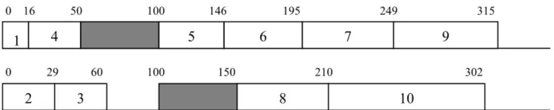
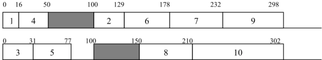
Example 3.1: Consider two-parallel machine case and the following 10-job problem with processing times as shown in Table 3-1, and without loss of generality assume that jobs are indexed in SPT order.
Table 3-1: Processing times of jobs
job i 1 2 3 4 5 6 7 8 9 10
pi 16 29 31 34 46 49 54 60 66 92
Starting time of unavailability in the first machine is 50, that in the second machine is 100, and duration of unavailability on both machines is 50. Define schi is the assignment of job i that is the interval job i
assigned.
The NS algorithm starts with the initial solution shown in Table 3-2.
Table 3-2: Initial solution
job i 1 2 3 4 5 6 7 8 9 10
schi 1 3 3 1 2 2 2 4 2 4
The value for this initial solution is 1572. Once again, since the SPT order is maintained within each interval, the search process consists in reassignment of certain jobs to different intervals. A graphical illustration of the initial schedule given in Table 3-2 is shown in Figure 3-8. j C
∑
0 16 50 100 146 195 249 315 9 7 6 5 4 1 0 29 60 100 150 210 302 10 8 3 2No idle time is incurred on machine 1, and the total idle time on machine 2 is 40 time units in interval 3.
The Neighborhood Search algorithm looks for a one- or two-job exchange between sub-neighborhoods defined above. Job exchanges are performed by selecting two jobs from each interval and interchanging their assigned intervals. Initially we add a dummy job to each interval with processing time 0 to allow two- and three- way job exchanges. Let d1, d2, d3, and d4 be the dummy jobs numbered with respect to the interval they assigned. The algorithm starts by selecting the sub-neighborhood that considers only the job exchanges between interval 1 and 3. Then it considers all possible job pairs for a potential exchange operation. Since no job exchanges result in a reduction in the
∑
value, the algorithm passes on to sub-neighborhood that considers the job exchanges between intervals 2 and 3. Then it selects jobs d2, and 5 from interval 2 and jobs d3 and 2 from interval 3 for an exchange operation. Since this exchange results in both an improvement in the objective function value, and a reduction in the idle time on machine 2, it is accepted and new schedule becomes as shown in Table 3-3.j C
Table 3-3: Schedule obtained after the first move
job i 1 2 3 4 5 6 7 8 9 10
sch i 1 2 3 1 3 2 2 4 2 4
A graphical illustration of this new schedule is displayed in Figure 3-10.
0 16 50 100 129 178 232 298
1 4 2 6 7 9
0 31 77 100 150 210 302 Figure 3-10: Schedule obtained after first move
10 8
The value of this new schedule is 1523. The search mechanism is then recentered around this solution and the process restarts by taking the first two jobs from each interval. These jobs are jobs d2 and 2 from interval 2 and jobs d3 and 3 from interval 3. Exchanging these particular jobs does not yield a better solution, and hence this exchange is rejected. Then jobs in the 1
j C
∑
st and the 3rd place from interval 2 (d2 and job 6) and
first two jobs from interval 3 (d3 and job3) are considered. It is calculated that exchanging these jobs yields a feasible solution and improves the objective function and also this exchange decreases the idle time on machine 2. Then this exchange is accepted and new schedule becomes
Table 3-4: Schedule obtained after the second move
job i 1 2 3 4 5 6 7 8 9 10
schi 1 2 2 1 3 3 2 4 2 4
And the assignments graphically become
0 16 50 100 129 160 214 280 0 46 95 100 150 210 302 10 8 6 5 9 7 3 2 4 1
Figure 3-11: Schedule obtained after second move
New objective value is 1502. The algorithm initializes the search and starts with the first two jobs from the interval. When search is completed in sub-neighborhood intervals between 2 and 3, the algorithm continues with sub-neighborhoods between intervals 1-4, 1-2, 3-4, 1-4, 4-1-2, 2-3-4, 4-3-2, and 2-4. When no exchange can be found within these sub-neighborhoods the algorithm turns to sub-neighborhood 1-3 and starts searching for improving moves. When there is no improving move in all of the 10 sub-neighborhoods the algorithm stops. In our example NS
algorithm gives 1497 as the objective value at the end, that is found in branch-and-bound algorithm as the optimal value.
Computational Complexity
The algorithm generates C(2m,2) + 2m×C(m,2) sub-neighborhoods in a problem where m is the number of machines. Search of a sub-neighborhood has a complexity of n5m log m where n is the number of
jobs. Hence, searching the whole neighborhood once has a complexity of
n5m4 log m. The algorithm repeats searching whole neighborhood until
no improving move can be found. Then this repeating action has a complexity of n2, because
∑
Cjvalue cannot exceed(
1)
2 n+ n j C
∑
pmax andevery movement results in an integral decrease in value. Therefore, the NS algorithm has a computational complexity of n7m4 log m.
3.4.2.3. Simulated Annealing Application
This algorithm uses the same neighborhood structure adopted in algorithm NS. It is different, however, in that in addition to always accepting those moves that result in a reduction in the objective value, it also accepts moves that result in an increased
∑
Cj value with some probability. In this way, it allows for searching different valleys in an attempt to avoid entrapment at a local optimum.The algorithm is a straightforward application of the classical approach proposed by Kirkpatrick et al. [28]. Recall that in algorithm NS, a job exchange is accepted only if:
1. it decreases the idle time on machines 1 and 2, and 2. it results in a smaller objective value.
The simulated annealing algorithm entirely disregards the first condition while extending the second condition by also allowing moves that increase the objective value with a certain probability. In particular, a move that results in an increase in the
∑
Cj value can be accepted with a probability of t t e ∆ −where ∆t is the magnitude of the resulting increase and t is the current temperature of the system.
The parameters of the simulated annealing algorithm such as the initial temperature, cooling function, and maximum number of iterations are set based on preliminary experimentation. The initial temperature is set as 100. A linear cooling function f(t)=0.99t is adopted. The maximum number of iterations to be performed at a given temperature is set at 100 for each neighborhood. Finally, the system is considered frozen when temperature of the system fell below 0.1, that the algorithm is terminated when tfin 0.1. A pseudo code of the algorithm is shown below. ≤
Let V be the set of neighborhoods constitutes the whole neighborhood and Ej’s be the elements of this set,
(1) W = ∅;
(2) Select a sub-neighborhood Ej s.t. Ej∉W; W=W E∪ j; set i = 1;
(3)Consider a job-pair exchange; ∆t:= change in the objective value; (4) if ∆t <0, perform exchange; go to (7);
(5) R~U(0,1); if ∆t >0 and e− ∆( / )t t > R, go to (7);
(6) Reject exchange; if all pairs are not considered go to (3); else go to (9); (7) Perform exchange; i = i + 1;
(8) If i < iterations, go to (3);
(9) if W = V, t = 0.99t; go to (10), else go to (2) ; (10) if t ≤ 0.1, exit;
3.5. COMPUTATIONAL
EXPERIMENTATION
In this section, we develop an experimental design framework and analyze the performance of the proposed algorithms via computational experimentation on the 2-machine case of the problem.
3.5.1. EXPERIMENTAL DESIGN
Processing times of jobs are generated from a uniform distribution between 1 and 100, and the duration of each period of unavailability is set equal to the average processing time of 50.
Starting times of unavailability periods in each machine is taken as experiment variable. The starting time of the period of unavailability on each machine is set systematically as early, medium, and late as shown in Table 3-5. For the first machine, early start of unavailability is 5n, medium start of unavailability is 25n/2, and late start of unavailability is 20n where n is the number of jobs. For the second machine, early start of unavailability is immediately after the end of period of unavailability on the first machine. Medium start of unavailability gives a gap of two unavailability durations after the end of the unavailability period on the first machine and late start of unavailability gives a gap of four unavailability durations after the end of the unavailability period in the first machine. The starting times and durations of unavailability periods are: