INTEGRATING BIOLOGICAL PATHWAYS
AND GENOMIC PROFILES WITH CHIBE 2
a thesis
submitted to the department of computer engineering
and the graduate school of engineering and science
of bilkent university
in partial fulfillment of the requirements
for the degree of
master of science
By
Merve C
¸ akır
I certify that I have read this thesis and that in my opinion it is fully adequate, in scope and in quality, as a thesis for the degree of Master of Science.
Assoc. Prof. Dr. U˘gur Do˘grus¨oz(Advisor)
I certify that I have read this thesis and that in my opinion it is fully adequate, in scope and in quality, as a thesis for the degree of Master of Science.
Assist. Prof. Dr. Can Alkan
I certify that I have read this thesis and that in my opinion it is fully adequate, in scope and in quality, as a thesis for the degree of Master of Science.
Assist. Prof. Dr. ¨Ozlen Konu
Approved for the Graduate School of Engineering and Science:
Prof. Dr. Levent Onural Director of the Graduate School
ABSTRACT
INTEGRATING BIOLOGICAL PATHWAYS AND
GENOMIC PROFILES WITH CHIBE 2
Merve C¸ akır
M.S. in Computer Engineering
Supervisor: Assoc. Prof. Dr. U˘gur Do˘grus¨oz July, 2013
Biological pathways store information about spatial and temporal organiza-tion of interacorganiza-tions taking place in an organism. They hold valuable informaorganiza-tion that can assist scientific community in understanding the details of a particular mechanism or deciphering the reasons of disruption when the system goes wrong. However, extracting knowledge from these pathways is not trivial as they can be huge and complicated. Additionally, simple visualization of pathways will only reveal limited knowledge, whereas their integration with experimental results can identify distinct and intriguing relationships. Therefore, it is critical to have tools that are specialized in analyzing and understanding biological pathways.
ChiBE is one such tool that can visualize, manipulate and analyze pathway data stored in BioPAX format. While preparing the second version of the tool, there have been improvements regarding pathway searches, high throughput data integration, and database connections. Visual notation has also been updated in order to follow standards in visualizations defined by the SBGN community.
Previously defined pathway query algorithms have been adapted to be com-patible with the BioPAX model. New query types have also been designed to offer a wider range of options. With these queries, ChiBE now offers a variety of ways of pathway decomposition and thorough analysis of complex pathway views. There has also been improvements in integration of high throughput experi-mental results. To offer easy access to expression microarrays, a gateway to the GEO database has been added. The cBio Cancer Genomics Portal is also now reachable within ChiBE in order to obtain information about genomic status of various cancer cells. After simply asking for an identifier of a particular experi-ment, ChiBE retrieves the results from databases and then integrates them with
iv
the available pathway view through color codes. Furthermore, a connection to DAVID database is available, in case users want to annotate a list of genes with respect to biological terms associated with them.
With these new features and improvements, ChiBE 2 has become a compre-hensive tool that offers a wide range of analysis options with a genomics-oriented workflow to deepen our understanding of biological pathways.
Keywords: Computational biology, bioinformatics, pathway informatics, pathway visualization, genomics.
¨
OZET
B˙IYOLOJ˙IK YOLAKLARIN VE GENOM˙IK
PROF˙ILLER˙IN CHIBE 2 YOLUYLA ENTEGRASYONU
Merve C¸ akır
Bilgisayar M¨uhendisli˘gi, Y¨uksek Lisans Tez Y¨oneticisi: Do¸cent Dr. U˘gur Do˘grus¨oz
Temmuz, 2013
Biyolojik yolaklar bizlere bir organizmanın devamlılı˘gını sa˘glayan et-kile¸simlerin mekansal ve zamansal organizasyonu hakkında bilgiler sunabilir. Bu yolaklar, bilim d¨unyasına ¨onemli bir biyolojik mekanizmayı daha detaylı anla-masında veya sistemde g¨ozlenen bir sorunun sebebinin anla¸sılmasında ¨onemli katkıda bulunabilirler. Fakat yolaklar b¨uy¨uk ve karma¸sık olabilecekleri i¸cin, on-lardan bilgi elde etmek basit bir i¸slem de˘gildir. Ayrıca sadece g¨orselle¸stirme odaklı analizler bizlere sınırlı miktarda bilgi sa˘glayabilirken, bu g¨orsellerin deneysel sonu¸clar ile entegre edilmesi farklı ve ilgin¸c etkile¸simleri a¸cı˘ga ¸cıkarabilir. Bu ne-denle, biyolojik yolakların analizi ve daha detaylı anla¸sılması ¨uzerine yo˘gunla¸smı¸s yazılım ara¸clarına sahip olmanın ¨onemi b¨uy¨ukt¨ur.
ChiBE, BioPAX formatında saklanan yolak verilerinin g¨orselle¸stirilmesi, d¨uzenlenmesi ve analizi ¨uzerine odaklanmı¸s bir yazılım aracıdır. Yazılımın ikinci versiyonu geli¸stirilirken ¸cizge ¨uzerinde aramalar, y¨uksek ¸cıktılı deney sonu¸clarının entegrasyonu ve veritabanı ba˘glantılarının sa˘glanması ¨uzerine yo˘gunla¸san ek-lemeler yapıldı. Ayrıca ChiBE’nin g¨orsel sembolleri de SBGN tarafından be-lirlenmi¸s standartları takip edecek ¸sekilde g¨uncellendi.
Daha ¨onceden tanımlanmı¸s olan yolak sorgulama algoritmaları BioPAX mo-delleri ¨uzerinde kullanılabilecek ¸sekilde uyarlandı. Bunlara ek olarak yeni yolak sorgulama t¨urleri de geli¸stirildi. Bu algoritmaların eklenmesiyle birlikte, ChiBE artık yolakları daha k¨u¸c¨uk par¸calara ayrı¸stıran ve karma¸sık ¸cizgelerin detaylı analizini sa˘glayan bir¸cok farklı yola sahip oldu.
Y¨uksek ¸cıktılı deneylerin sonu¸clarının ¸cizgeler ile entegrasyonu ile ilgili de bazı iyile¸stirmeler yapıldı. Mikrodizi deneyleri sonu¸clarına kolay eri¸sim sun-mak i¸cin GEO veritabanına ula¸sım noktası eklendi. Ayrıca, kanser h¨ucrelerinin
vi
genomik durumu hakkında bilgi sunmak i¸cin ‘cBio Cancer Genomics Portal’ı da ChiBE i¸cerisinden eri¸silebilir hale getirildi. Kullanıcıdan deney verisini be-lirleyen bilgiyi aldıktan sonra, ChiBE ¨oncelikle istenilen deneyin sonu¸clarını ve-ritabanından elde eder ve ardından bu sonu¸cları ¸cizge ile renk kodları kullanarak entegre eder. Bunlara ek olarak, DAVID veritabanına da kolay bir eri¸sim sunul-maya ba¸slandı. B¨oylelikle, kullanıcılar bir gen listesini bilinen biyolojik terimlerle e¸sle¸stirme ¸sansına sahip olacaklar.
Bu yeni ¨ozellikler ve iyile¸stirmelerle birlikte ChiBE 2 genomik odaklı i¸s akı¸sına elveri¸sli, geni¸s ¸capta analiz se¸cenekleri sunan ve biyolojik yolaklar hakkındaki bilgi birikimimizi derinle¸stirebilecek kapsamlı bir yazılım aracı haline geldi.
Anahtar s¨ozc¨ukler : Hesaplamalı biyoloji, biyoenformatik, yolak g¨orselle¸stirmesi, genomik.
Acknowledgement
First of all, I would like to thank to my advisor Assoc. Prof. Dr. U˘gur Do˘grus¨oz who has been a great mentor to me for many years. I am grateful to him for giving me the chance and courage to pursue this path, then guiding and supporting me through it.
¨
Ozg¨un Babur deserves special thanks as I have learned a lot from him about ChiBE and received significant advice and support from him while working on ChiBE. I want to thank Arman Aksoy for his contribution in parts related with the cBio Cancer Genomics Portal and Emek Demir for his feedbacks and opinions related to ChiBE.
Assist. Prof. Dr. Ozlen Konu and Assist.¨ Prof. Dr. Can Alkan have reviewed this thesis, so I would like to thank them for their valuable opinions and for helping me improve my thesis.
I would also like to thank to the Scientific and Technological Research Council of Turkey, T ¨UB˙ITAK, for their support.
This journey would have been harder to complete if I did not have the support from my friends. I would like to express my gratitude to all of them, including but not limited to i-Vis Research Group members - Mecit, C¸ a˘gda¸s, Beg¨um, ˙Istemi, Marzie, Onur - Salim, Muhsin Can, Shatlyk, all my “molecular biologist” friends especially Damla and Derya. Finally, I would like to thank to my family for their support and understanding.
Contents
1 Introduction 1
1.1 Biological Pathways . . . 1
1.2 Standards for Pathway Data Exchange . . . 5
1.3 Contribution . . . 8
2 Background Information 10 2.1 Graphs . . . 10
2.2 Pathways . . . 11
2.3 Network Traversal and Querying . . . 13
2.3.1 Breadth-First Search . . . 13
2.3.2 Neighborhood Query . . . 14
2.3.3 Paths Of Interest . . . 15
2.3.4 Graph Of Interest . . . 16
2.3.5 Common Stream Query . . . 17
CONTENTS ix
2.4.1 Cytoscape . . . 18
2.4.2 PathVisio . . . 19
2.4.3 CellDesigner . . . 21
3 Graph Queries 23 3.1 Adapting Breadth-First Search . . . 24
3.2 Compartment Query . . . 28
3.3 Path Iteration Query . . . 30
3.4 Adapting Query Algorithms . . . 32
3.4.1 Neighborhood Query . . . 32
3.4.2 Paths From To Query . . . 34
3.4.3 Paths Between Query . . . 37
3.4.4 Common Stream Query . . . 38
3.5 Pathway Commons Queries . . . 39
4 High Throughput Data Integration 42 4.1 Fetch From GEO . . . 42
4.1.1 Implementation of Fetch From GEO Feature . . . 44
4.2 Fetch From cBioPortal . . . 50
5 Further Improvements 55 5.1 Connecting to DAVID . . . 55
CONTENTS x
5.2 SBGN-PD Notation . . . 58
6 Example Results 61
6.1 From Pathway View to Genes of Interest . . . 61 6.2 Comparison of Experimental Results . . . 67 6.3 Expansion of Experimental Results . . . 71
7 Conclusion 74
7.1 Comparing ChiBE with Other Tools . . . 76 7.2 Future Work . . . 76
List of Figures
1.1 A sample pathway obtained from KEGG database . . . 3
1.2 A sample pathway image integrated with microarray experiment result. The color codes are based on the experimental values each gene is associated with. . . 4
1.3 A sample SBGN process description map describing the events occurring in a neuro-muscular junction. . . 7
2.1 A sample graph from ChiBE . . . 11
2.2 Different glyphs supported by ChiBE to represent different biolog-ical entities and relationships [35] . . . 12
2.3 Sample pathway views obtained with Cytoscape . . . 19
2.4 Sample pathways obtained with PathVisio . . . 20
2.5 Sample pathways obtained with CellDesigner . . . 22
3.1 Sample graphs to highlight the differences observed due to BioPAX structure . . . 24
3.2 Structures of BioPAX that causes problems during application of BFS . . . 25
LIST OF FIGURES xii
3.3 An alternative distance labeling approach designed to overcome
the problems . . . 26
3.4 An example result for Compartment query . . . 29
3.5 An example result for Path Iteration query . . . 31
3.6 An example result for Neighborhood query . . . 33
3.7 An example result for state-based Neighborhood query . . . 34
3.8 An example result for Paths From To query . . . 35
3.9 An example result for Paths Between query . . . 38
3.10 An example result for Common Stream query . . . 39
3.11 A sample result of Pathways With Keyword query . . . 40
4.1 Sample “Fetch From GEO” dialog . . . 43
4.2 A portion of a platform file GPL96 . . . 45
4.3 A portion of known reference set that is stored in ChiBE listing the generic name and synonyms for popular references . . . 46
4.4 A portion of a series matrix file GSE6014 . . . 46
4.5 A portion of .ced file highlighting its components . . . 48
4.6 Example pathway view with microarray data (GSE6014) mapped onto the pathway objects . . . 49
4.7 cBio Portal parameter selection dialog . . . 52
4.8 cBio Portal Settings dialog where you can adjust thresholds for different data types . . . 53
LIST OF FIGURES xiii
4.9 A sample pathway overlayed with data from the cBioPortal, also exemplifying the cBioPortal Data Details Dialog of a selected node. 54
5.1 A sample pathway image used to connecting to DAVID, along with the dialog that will be used for selection of analysis option. . . 57 5.2 The result of “Gene Name Batch Viewer” analysis . . . 58 5.3 SBGN-PD’s visual notation (modified from [16]) . . . 59
6.1 Signaling by FGFR pathway is integrated with expression data. “Highlight With Data Values” dialog can also be seen, reflecting the smallest and largest expression values found in the experiment. 63 6.2 IL17RD and MAP2K1 entities, which are highlighted in yellow,
are found to be the outliers of this expression dataset. . . 64 6.3 Signaling by FGFR pathway is integrated with alteration data.
“Highlight With Data Values” dialog can also be seen, reflecting the smallest and largest alteration percentages found in the exper-iment. . . 65 6.4 EGF, which is highlighted in yellow, is found to be the entity
with highest alteration percentage. The details of genomic changes observed in EGF can be seen in “EGF: Data Details” dialog. . . . 66 6.5 A portion of the result of functional annotation analysis performed
with DAVID using IL17RD, MAP2K1 and EGF . . . 67 6.6 Path from CDKN2A to RB1 is integrated with alteration values
of glioblastoma samples. . . 69 6.7 Path from CDKN2A to RB1 is integrated with alteration values
LIST OF FIGURES xiv
6.8 A simple network displaying the identified path along with alter-ation percentages [35] . . . 72 6.9 The paths from ERBB2 to KRAS with length 1 are integrated with
Chapter 1
Introduction
1.1
Biological Pathways
Cells, the tiny building blocks of living organisms, can be seen as a huge factory filled with metabolites, proteins or nucleic acids that are in constant interaction with each other to keep the factory running. Understanding details of these mech-anisms and sets of interactions in its full context is a challenging task. Therefore rather than dealing with the whole set, researchers opted to divide cellular events into smaller yet meaningful pieces. This smaller set of interactions are chosen to be bound together as they contain molecules having causal relationships with each other, in the end to accomplish a biological event. This set of meaningful interactions is called pathways [1].
With the advances in molecular biology field, our knowledge in cellular events and pathways has vastly increased. With ongoing experiments, missing pieces in cellular machinery are being completed which leads to a more and more compre-hensive state of knowledge in biological pathways. After deciphering the com-ponents of a pathway, the next step is more detailed analysis of this pathway in order to fully understand its function, discover its relationship with other path-ways or study the possible outcomes when the machinery of the pathway goes wrong. This means that the focus of research is now diverting from gene level
to pathway level, which mandates the development of approaches that will aid scientific community in this quest.
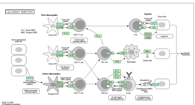
One of the first steps of pathway analysis is the visualization of a pathway. The details of a pathway deciphered through experiments can be transmitted to other researchers through textual descriptions (Figure 1.1(a)). However, long and complicated texts can make it harder to follow the interaction path and extract the critical points of the pathway. Instead, a visual representation can ease this communication. In Figure 1.1(b), we see a visualization obtained from KEGG database [2] of the textual description seen in Figure 1.1(a). With this visual representation, it is much easier to follow the flow of events. Also thanks to spatial organization, it is only trivial to find a subset of interactions, whereas one would have to scan the whole text to find the same information. This is just one instance reflecting the importance of proper choice of representation in easing the pathway analysis steps.
Unfortunately, this simple conversion of text into a diagram is not enough. One of the biggest problems associated with this is the fact that it is a static image. This means that you are limited to knowledge offered by the image and you cannot expand it or focus on a subpathway of the original image. Therefore, the advantages of this static image representation is limited. We need further improvements in pathway visualization approaches in order to be able to perform progress in research through them. There are many different approaches that can be followed to convert these static images into better analysis devices. For instance, being able to crop a pathway to generate a smaller subpathway or hiding unnecessary nodes and edges can enable researchers to focus on the pieces of a large pathway that attracts their attention most [3, 4, 5]. Alternatively, query operations can be performed on the pathway or on pathway databases [6, 7]. With such options, users can start with a set of molecules in hand and search them and their interactions in the pathway in order to generate a subpathway focusing on the molecules of interest and their relationships. Multiple different layout options can be offered, which can help the user arrange the topology of image in hand in order to understand the spatial organization of the pathway better [4, 5].
(a) Textual description of a biological pathway
(b) Visual representation of the same pathway
Figure 1.1: A sample pathway obtained from KEGG database
Figure 1.2: A sample pathway image integrated with microarray experiment re-sult. The color codes are based on the experimental values each gene is associated with.
All these exemplify the cases of extension of analysis through changes in path-way structure or topology. Another trail of approach is the integration of exper-iment results with pathway knowledge [3, 6, 8]. Traditional way of analyzing high throughput experiment results is gene-centric. For instance, to make use of results of microarray experiments, researchers tend to identify genes that are significantly differentially expressed from rest of the gene set. Although this re-turns a set of genes that can be building blocks of new hypotheses, one can gain a greater amount of knowledge from these experiments if pathway knowledge is also added to the equation. Integrating high throughput experiment results with pathways generates new pathway images that not only reflect the interactions be-tween molecules but also their experimental conditions (Figure 1.2). Researchers will be able to see whether there are clustered overexpressed molecules or if there is a dysregulated transcription factor causing differential expression in molecules in its downstream. With this approach, we can increase the amount of knowledge we can extract from both pathway information and experiment results. The set of experiments that is suitable for this integration is not limited to microarray experiments. Sequencing experiments that reflect the alteration status of genes
or copy number variation experiments are some of other cases that possess the advantage of being analyzed at a pathway level.
Pathway visualization and analysis field is still open to developments that includes but not limited to the ones discussed above. Answering the needs of the field in these respects is an important step in ensuring full knowledge acquisition from pathway information reconstructed from biological experiments.
1.2
Standards for Pathway Data Exchange
The shift of focus from gene-centric approaches to pathway-centric approaches has resulted in a rapid increase in the amount of available pathway data. Lots of different research groups focused on reconstructing pathways from biological experiments and knowledge. One problem associated with this expansion is the lack of compatibility between different curators. Due to lack of a standard format and notation for generation of pathway data, different research groups have come up with different ways of storing and representing pathway data. This builds a barrier in front of the hopes of combining data from different resources in order to build a comprehensive resource. It also makes it harder for users to utilize this data as they will need to adjust to a new way of representation every time they want to use data from a different source.
To overcome these problems, some community efforts have emerged to stan-dardize pathway data storage and representation. One of them is Biological Pathway Exchange (BioPAX), whose objective is to develop a standard format for storing and sharing pathway data [1]. This community effort has been ini-tiated in order to define a standard syntax for representation of pathway data, which will in turn remove the barriers in collecting, storing and sharing them. The developed syntax is based on OWL (Web Ontology Language). The initial stages of the project, called Level 1, only supported metabolic pathways. Then each level expanded the capabilities of the standard. Level 2 added signaling pathways and molecular interactions on top of metabolic pathways. The latest
version, which is Level 3, can additionally represent gene regulatory networks and genetic interactions. With this standardization, one of the biggest communication barrier between pathway researchers has been eliminated.
The followup to a standard in storage format is a central database storing and offering pathway data in that format. Pathway Commons project has started to answer this demand [9]. The main aim of this effort is to build a central hub for reaching pathway data stored in BioPAX format. Pathway data that is already stored in several different databases are collected together and integrated to be stored in one database. Pathway Commons offers different ways of reaching to this data. Users can simply use their web site in order to search for specific pathways. Download site can be used for bulk downloads of integrated set of pathway data and web service is offered to software developers as a connection to the database that can be used in their software. With these offerings, researchers can easily reach to a comprehensive set of already available pathway data in the standard format of BioPAX.
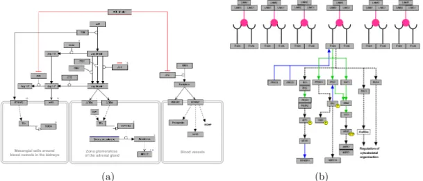
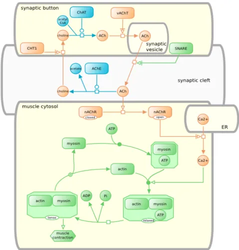
The problem of storing pathway data in a standard format and database has been solved, yet there still are points needing consideration: the visualization of this standard data. BioPAX and Pathway Commons have helped researchers share pathway data with each other without considering compatibility or under-standability problems. However there was still no standard in visualizing this data. If everyone was to come up with their own notation for visualization, then it would be problematic for the end user to familiarize with all these different notations. Thus a standard way of representation was required and Systems Bi-ology Graphical Notation (SBGN) project has been born for this reason [10]. The purpose of this effort is to develop standard notations for visualizing biological processes. SBGN community have developed three different languages for rep-resentation of biological pathways: process description, entity relationship and activity flow. Figure 1.3 shows an example for process description language, in which the events observed in a neuro-muscular junction are visualized with a fo-cus on interactions taking place [11]. These languages form a comprehensive and unambigous way of representing pathway data.
Figure 1.3: A sample SBGN process description map describing the events oc-curring in a neuro-muscular junction.
All these efforts have helped significantly in building a pathway research com-munity that stores, shares and represents pathway data in a centralized and understandable way. This in turn has helped software developers to stop being concerned about these matters and to start focusing on developing tools that will answer the needs of pathway informatics field that has been discussed above.
1.3
Contribution
ChiBE is an open source tool that specializes in visualization and analysis of pathway data stored in BioPAX format [3]. Its first version is capable of visu-alizing BioPAX Level 2 pathway data, supporting on-demand layout of loaded pathway views. The tool offers various features that can help researchers in their analysis of BioPAX formatted pathways, including cropping subpathways, high-lighting particular elements in pathways or creating simple interaction views. It can access Pathway Commons to reach the neighborhood of a specific molecule and perform a mapping between high throughput experiments and pathway view through user input.
Although it offers such a wide range of features, there is still room for im-provement to make ChiBE more useful to scientific community. We wanted to improve the tool in such a way that it will offer a variety of features that can help the researchers to analyze BioPAX formatted pathway data from different perspectives. The remainder of this thesis will focus on new methods and im-provements to existing methods and their implementation in ChiBE, which can be summarized as follows:
• Breadth-first search algorithm has been tailored to the specific structures stored in BioPAX format. Using this search approach, previously defined query algorithms have been implemented [12]. (Chapter 3)
• New queries have been designed and implemented to offer users the flex-ibility of searching a pathway model based on a set of biological entities. (Chapter 3)
• A one-click access to GEO database [13] has been added to ease the inte-gration of expression microarrays with pathway view. (Chapter 4)
• Integration of cancer genomics data with pathway view based on alteration ratios of genes is now offered through the communication with the cBio Cancer Genomics Portal [14]. (Chapter 4)
• Connection to DAVID database [15] is supplied in order to offer a way of annotating and understanding a particular list of genes more thoroughly. (Chapter 5)
• Visual notation of ChiBE is updated in order to follow guidelines specified by SBGN [16]. (Chapter 5)
• Support for visualization of Level 3 BioPAX models is now provided, on top of the existing support for Level 2 models.
After discussing these improvements in detail in the specified chapters, Chap-ter 6 will focus on examples related to these features in order to highlight their use cases. Chapter 7 will conclude the thesis along with a discussion on future directions.
Chapter 2
Background Information
2.1
Graphs
A graph G can formally be defined as a pair of sets (V, E), where V stands for the non-empty set of nodes and E stands for the set of edges. Edge set E contains elements that connects nodes found in set V . e = {a, b} represents an edge joining node a and node b. Nodes a and b are incident to edge e. Additionally, the two nodes are neighbors of each other.
A non-empty subgraph P = (V0, E0) will be called as a path, if V0 and E0 follow the upcoming criteria. The node set V0 needs to be composed of {v0, v1, v2, ..., vn−1, vn}, with v0 and vn being the path’s endpoints. The edge
set E0 will be composed of edges connecting the nodes in V0, which are repre-sented as {v0v1, v1v2, ..., vn−1vn}. The length of path P is equal to the size of
edge set E0. For a path to be directed, all of the ordered edges have to have the same direction. A cycle will be formed if a path’s endpoints are the same node n. Relations between nodes based on their location on the path can also be defined. Let node n0 be the starting point of a directed path and node nk be its ending
point. Then this means that node nk is in downstream of node n0 and node n0 is
Paths can also be found between sets of nodes. Consider two node sets V1 and
V2. If only the endpoints of a path is found in V1 and V2and no other intermediate
nodes belong to these two node sets, then the path can be named as V1− V2 path.
Compound graphs refer to the cases where a node in the graph may contain other nodes and edges within it. On top of the sets of nodes V and edges E, a compound graph is also defined by a set of inclusion edges F . Inclusion set F is used to represent nesting relationships between a compound node and the node found within it, which can be called as child node.
2.2
Pathways
The realization of these concepts in pathway visualization context can be seen in Figure 2.1, which represents a sample pathway image from ChiBE. As it can be seen, a pathway view consists of nodes and the interactions between them.
Figure 2.1: A sample graph from ChiBE
nodes are used for two different purposes. They can either represent complexes composed of multiple entities, such as “MEK1:ERK-1” complex, or compartments corresponding to cellular localizations, such as cytoplasm. In the cases of com-plexes, child nodes of a compound node can only be other physical entity nodes. However, children of compartment compound nodes can be any of them, including other compound nodes. The remaining elements of node set are visualized with simple nodes and they can either be a distinct state of a physical entity, drawn with rounded rectangles or transitions between them, drawn with gray squares. Transitions signify the cellular events involving these biological entities, including complex formations, transportations or reactions such as phosphorylation.
The elements of edge set connect transitions and states interacting with them based on the type of relationship between these nodes. There are different types of edges used for different purposes, such as substrate, product, and effector edges. Black edges are used to represent substrate and product relationships, whereas green edges signify activating effectors and red ones are used for inhibitory effector edges. There are cases where more than one effector molecule is present or where an effector edge targets another effector edge. To represent these cases, control nodes drawn with gray diamonds are used. The complete set of node and edge types supported by ChiBE can be seen in Figure 2.2.
Figure 2.2: Different glyphs supported by ChiBE to represent different biological entities and relationships [35]
An example of a path can also be seen in Figure 2.1, which is highlighted in yellow. The start point of this path is the complex phospho-ERK-1:MEK1 and after going through two reaction nodes and a physical entity node MAP2K1, the path ends at the complex MEK1:ERK-1. In this graph, p-MEK1 is in the downstream of CDK1 and MEK1 is in the upstream of p-MEK1.
2.3
Network Traversal and Querying
2.3.1
Breadth-First Search
Breadth-first search [17] is a technique that has been developed to perform searches on graphs with respect to a set of nodes. Its main purpose is to identify the nodes in the graph that can be reached from the nodes found in a distinct source set. The basic logic of breadth-first is traversing every reachable node at distance k before moving onto the nodes found at distance k + 1. A sample breadth-first search algorithm is given in Algorithm 1.
Algorithm 1 BFS(S, T , dir, limit)
1: for all node n ∈ S do
2: n.color ← gray 3: n.label(dir) ← 0 4: Q ← ∅ 5: R ← ∅ 6: Q.enqueue(S) 7: while Q 6= ∅ do 8: current ← Q.dequeue()
9: if current.label(dir) < limit and current /∈ T then
10: N ← current.neighbor(dir)
11: for all node neigh ∈ N do
12: if neigh.color = white then 13: neigh.color ← gray 14: neigh.label(dir) ← current.label(dir) + 1 15: Q.enqueue(neigh) 16: current.color ← black 17: R ← R ∪ {current} 18: return R
The algorithm requires a source set of nodes (S) and a direction dir deter-mining whether the search should traverse the graph moving forwards from the source nodes or backwards. It also asks for a limit, which is an upper bound for a reachable node’s distance from the source set. A target set of nodes (T ) can also be defined and when the traversal reaches to an element from this set, it does not go further in that direction. To prevent passing over a particular node multiple times, a coloring scheme is used in breadth-first search implementations. At the beginning all nodes are white, except for the ones in source set. They have the color gray as it represents the nodes that are currently in queue. Once a node is reached for the first time, its color is converted from white to gray and it is placed in the queue. black is reserved for nodes that have already been processed. The complexity of this algorithm is O(|V | + |E|), linear in the number of nodes and edges.
This search algorithm will become useful when we need to move through a graph in order to perform queries focusing on a set of nodes found in the graph.
2.3.2
Neighborhood Query
Finding the nodes surrounding a particular node is one of the first aspects that comes to mind while trying to extract knowledge from that node using the given graph. Therefore one of the basic uses of graph traversal algorithms is querying the neighborhood of a particular node [12].
Details of a proposed neighborhood query algorithm can be seen in Algo-rithm 2. The algoAlgo-rithm requires a set of source nodes (S), a traversal direction (dir), and a stop distance (limit). The search can be done in either downstream or upstream direction of source nodes or alternatively a combined search can be performed to get the complete neighborhood. If that is the case, two differ-ent breadth-first searches are performed, one in forwards and one in backwards direction. The target set of these searches are empty because there is no destina-tion; the search is simply bounded by the distance from the source nodes. The algorithm runs in O(|V | + |E|) time.
Algorithm 2 Neighborhood(S, dir, limit)
1: R ← ∅
2: if dir = fwd or dir = both then 3: R ← R ∪ BFS(S, ∅, fwd, limit) 4: if dir = rev or dir = both then 5: R ← R ∪ BFS(S, ∅, rev, limit) 6: return R
When implemented, this algorithm can easily be used to identify the set of nodes that are found within a certain distance from the set of source nodes. This way we can get more information about the characteristics of surroundings of these source nodes.
2.3.3
Paths Of Interest
When you have two different sets of nodes of interest, the directed paths between them whose endpoints are these two sets respectively can hold valuable informa-tion about the flow of interacinforma-tion between these sets. Similar to neighborhood query, a breadth-first traversal can be used for identification of these paths. The traversal needs to start from one of the sets and continue until it finds all the paths arriving to the nodes of the second set [12].
Algorithm 3 PathsOfInterest(S, T , limit)
1: C ← BFS(S, ∅, fwd, limit) 2: ResetColor(C)
3: C ← C ∪ BFS(T, ∅, rev, limit) 4: R ← ∅
5: for all node n ∈ C do
6: if n.label(fwd) + n.label(rev) ≤ limit then 7: R ← R ∪ {n}
8: return R
Algorithm 3 reflects the basics of a sample algorithm that follows the proposed reasoning to solve this problem. The algorithm requires a source set S from which the paths will start, a target set T to which the paths will converge and a distance
limit specifying the distance between source and target nodes. At first, a breadth-first search is performed with source set of nodes in forwards direction. This will be followed by a backwards directed search from target set of nodes. The resulting set of nodes will be composed of the ones whose sum of distance labels from these two queries does not exceed the search limit. This algorithm’s time complexity is O(|V | + |E|). With this approach, we will be able to recover paths originating from a set of nodes and ending at a different set of nodes whose length is smaller than a predefined threshold.
2.3.4
Graph Of Interest
A special version of the described Paths of Interest query approach can be used to solve a more general problem. Instead of identifying paths following a particular direction, we can identify all of the paths found between the elements of a set of nodes [12]. Rather than dividing the set into start point nodes and end point nodes, in this case we look for a comprehensive set of paths found within all elements of a single set.
Algorithm 4 simply shows how Paths of Interest query can be used for this query type. Rather than specifying a source set and target set, a single set of nodes is given to the algorithm as both source and target sets. As a result, we will be searching for the paths that start at one of the source nodes and ends at another source node. A search limit is also required to bound the length of the recovered paths. The complexity of this algorithm is clearly the same as Paths Of Interest, which is O(|V | + |E|).
Algorithm 4 GraphOfInterest(S, limit)
1: return PathsOfInterest(S, S, limit)
When Paths Of Interest query is run on the pathway in this way, we will be able to recover the ways to traverse the graph between the given set of nodes, irrespective of the direction.
2.3.5
Common Stream Query
Each node’s neighborhood holds special information for that particular node, however there may be even more valuable information hidden in the shared neigh-borhood of a set of nodes [12]. Searching for the elements that are located in the common downstream of a set of nodes will signify the point that the paths of these different nodes merge with each other. Nodes in the upstream that are commonly shared can be used to identify the point of divergence of different paths.
Algorithm 5 CommonStream(S, dir, limit)
1: C ← ∅
2: R ← ∅
3: for all node n ∈ S do
4: BF SRun ← BFS({n} , ∅, dir, limit) 5: for all node res ∈ BF SRun do
6: res.reached ← res.reached + 1
7: C ← C ∪ BF SRun
8: ResetLabel(BF SRun, dir) 9: ResetColor(BF SRun) 10: for all node c ∈ C do
11: if c.reached = S.size then
12: R ← R ∪ {c}
13: return R
Algorithm 5 explains the details of the algorithm that has been designed to find the upstream or downstream elements that are shared by a set of nodes. For every node in the source set S, first a breadth-first search is performed in the direction specified (dir) and bounded by the search limit. The difference of this algorithm from the previously discussed ones will be the way of determining final result set. For each node, a count called reached is kept. This reflects the number of times a particular node is found to be in the result set of breadth-first searches. So after each search run, the reached count of every node in the result set is incremented. In the end, only the nodes whose reached count is equal to the size of source set are placed in the result set. This is because we only want to recover the nodes that can be reached through every single element of the source set. So, in the end obtaining nodes fulfilling this criteria will return us the nodes that are common to the traversal paths of source nodes in the specified direction.
The run time complexity of this algorithm is O(|S| × (|V | + |E|)).
2.4
Related Work
This section will focus on the tools that have been developed for enhancing the visualization and analysis of pathway data in order to give an insight about the current status of the field.
2.4.1
Cytoscape
Cytoscape is a generic visualization tool that can be used to draw, visualize and analyze networks [18]. The tool is useful for purposes of wide range of fields, ranging from computational biology to social networks. There are numerous different plugins that can extend and specialize functions of the tool.
For computational biology purposes, core Cytoscape offers importing of net-works in lots of different file formats including .owl for BioPAX, .sbml and .sbgn for SBML and .xml files. Additionally networks can be obtained from online databases such as Pathway Commons. For the visualization of these networks, Cytoscape offers many different layout algorithms, such as circular, grid, spring embedded or sugiyama layouts. Figure 2.3(a) displays a network obtained from Pathway Commons database, laid out with degree sorted circle layout.
One of the Cytoscape plugins called BiNoM [19] can be used to analyze and manipulate biological networks stored in standard systems biology file formats. The plugin can be used to import and export files in BioPAX Level 3 and SBML format. It also offers topological analysis, such as centrality calculations. A sam-ple BioPAX model’s representation with BiNoM can be seen in Figure 2.3(b). The difference in visualization preferences of Cytoscape and BiNoM is prominent. Whereas core Cytoscape only offers a simple interaction network displaying the relationships between molecules, BiNoM offers a hierarchical pathway structure
(a) A sample view from Cytoscape (b) Sample pathway view obtained with Cytoscape plu-gin BiNoM
Figure 2.3: Sample pathway views obtained with Cytoscape
along with reactions connecting different molecules, which reflects more informa-tion about the events occuring in the pathway.
Examples of other plugins include MetScape [20], which can be used to ana-lyze high throughput gene expression and metabolomics data. KeyPathwayMiner [21] also has a similar purpose; it is specialized in identifying significant subnet-works within a biological network by making use of gene expression data. En-richmentMap [22] can be integrated with Cytoscape if a user wants to see the results of gene set enrichment analysis as a network. These examples show that users can install different plugins in order to customize Cytoscape and make it compatible with their needs.
2.4.2
PathVisio
PathVisio is an open source tool for visualization and editing of biological path-ways [23]. The tool can import and export pathpath-ways stored in XML files and
.mapp files - which is a format specifically related to GenMAPP [24]. Addi-tionally, pathway images can be exported in .pdf, .png, .svg and .tiff formats. Users are not only dependent on the already available pathway data; generation of pathways from scratch is also possible through drawing options offered by the tool.
The visual notation of PathVisio is quite unique, as seen in Figure 2.4. The tool uses specialized structures to reflect extra information easily - such as the compartmentalization of different environments through extra rectangular nodes seen in Figure 2.4(a). Another sample visualization can be found in Figure 2.4(b), in this example the use of significantly different edges to connect interacting nodes draws the attention of the user.
(a) (b)
Figure 2.4: Sample pathways obtained with PathVisio
Apart from visualizing the biological pathways, PathVisio can also integrate expression data with the pathway image. User is required to perform the mapping between expression data file and the structure of integration mechanism. After that, the data is integrated with the view through color coding.
PathVisio’s functionality can be expanded through available plugins. Cur-rently, there are plugins that can be installed to enable data import and export in BioPAX Level 3 or to enable drawing pathway views with SBGN notation.
2.4.3
CellDesigner
CellDesigner is another modeling and visualization tool for biological networks [25]. SBML files are the format that has been preferred by CellDesigner, it can import and export pathway data stored in .sbml and .xml files. Public databases such as BioModels and PANTHER can also be used to import pathway data. Similar to PathVisio, it is possible to create your own pathway models through drawing capabilities offered by CellDesigner.
CellDesigner uses a customized visual notation that is quite similar to SBGN specifications (Figure 2.5(a)). However, it is also possible to convert the view into a version that completely follows SBGN guidelines (Figure 2.5(b)). The tool offers multiple different automatic layout options, including but not limited to hierarchic, circular, tree and organic layouts. Users can choose any of them to optimize the pathway view’s organization according to their needs.
The connections offered to external databases are not limited to pathway data import. Upon selection from the view, one can choose to connect to many different databases such as PubMed, Entrez Gene, UniProt or MetaCyc to get more information about the selected node.
CellDesigner is also extensible through plugins. For instance, BioPAX Export plugin can be used to export pathway models in BioPAX Level 3 format. An-other plugin is available for integrating microarray and proteomics data with the pathway.
(a) Default visualization notation of CellDesigner
(b) The same view, this time with SBGN notations
Chapter 3
Graph Queries
With the advances in biological research, the scientific community’s knowledge about biological relationships and pathways have shown an increase at a signif-icant pace. This in turn led to a signifsignif-icant increase in the knowledge stored in pathway structures and databases. The scope and comprehensiveness of empir-ical pathway data are increasing each and every day. However, there are some drawbacks of this obvious achievement. Increasing pathway size negatively im-pacts the ease of analysis. Smaller pathway models can be extensively analyzed after simply visualizing it. As the size of pathway gets bigger, it becomes more and more complex to analyze a graph by simply looking at it due to the crowd-edness of the resulting picture. This problem has motivated us to offer users a way of easing analysis of complex graphs. For this purpose, we have implemented graph query algorithms that will help the user to decompose the bigger picture into smaller and meaningful parts.
In this chapter, these query algorithms will be discussed in detail. As ex-plained in Section 2.3, graph querying algorithms require graph search approaches to traverse the graph. The given breadth-first search algorithm however is not directly applicable to pathway models visualized by ChiBE due to the nature of BioPAX format. So initially, the way breadth-first search algorithm has been adapted to overcome these problems will be discussed. Then, new graph querying approaches depending on this algorithm that are targeted for biological pathways
will be explained, which will be followed by the application of query algorithms discussed in Section 2.3 to ChiBE through use of adapted breadth-first search approach.
3.1
Adapting Breadth-First Search
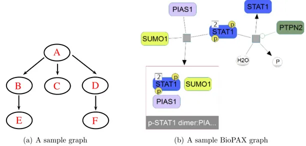
While performing queries on pathway models, we can try to use the breadth-first search given in Algorithm 1 in order to move through the pathway view and find distances between physical entities. However, this is not as straightforward as it seems. The regular BFS is a perfect match for graphs that contain one type of node connected with one type of edge (Figure 3.1(a)). However, the graphs dis-played with ChiBE are not that simple (Figure 3.1(b)). There are multiple types of nodes and edges. For instance, there are physical entity nodes represented with rounded rectangles and reaction nodes represented with gray squares. Dur-ing our search, we only want to focus on the distances between physical entity nodes, which means that there will be additional nodes between the nodes that we are interested in, causing problems in the calculation of distances.
A
B
C
D
E
F
(a) A sample graph (b) A sample BioPAX graph
Figure 3.1: Sample graphs to highlight the differences observed due to BioPAX structure
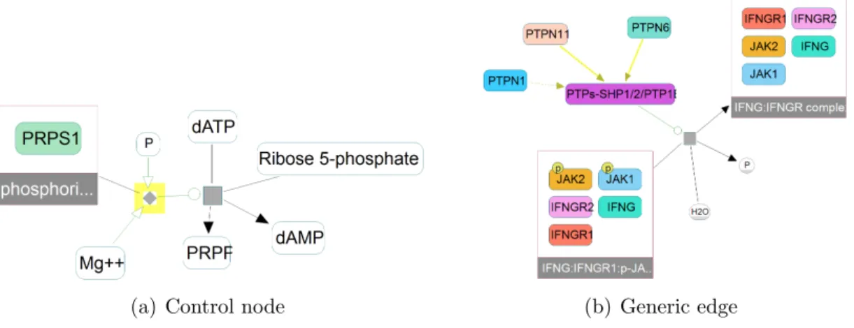
In the example seen in Figure 3.1(b), we see an alternating pattern between physical entity nodes and reaction nodes. A physical entity node is followed by a reaction node before connecting to the next physical entity node. BFS is still applicable to this graph with a simple change, which is multiplying the given distance limit with two. The kth physical entity from the source set will actually be at 2k distance from the source due to the presence of reaction nodes and with the multiplication, we will be searching within 2k distance boundaries and be able to identify physical entities at k distance as desired. Unfortunately, this pattern is not observed in all BioPAX models. There are cases where a reaction node is not followed by a physical entity node, as highlighted in Figure 3.2(a). Additionally, there is a special type of edge that represents generic relationships between nodes, which refers to the cases where a set of physical entities can be represented with a single generic version of them. In these cases, a physical entity node is directly connected to another physical entity node omitting a reaction node in between (Figure 3.2(b)). As a result of these special cases, we cannot apply the regular breadth-first search algorithm to calculate the distance between physical entity nodes.
(a) Control node (b) Generic edge
Figure 3.2: Structures of BioPAX that causes problems during application of BFS
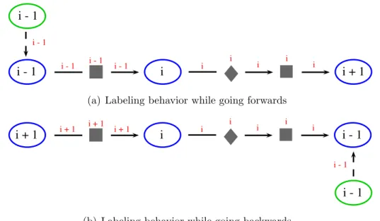
To overcome this problem, we have come up with a new way of calculating the distances while traversing the graph (Figure 3.3). As we want to see the distance between physical entities, we will be updating the distance labels only when we interact with a physical entity node - which from now on will be called as breadth
node. If we are traversing the graph in forwards direction, then the distance label will be updated only if the search enters a breadth node (Figure 3.3(a)). While traversing in backwards direction, distance will be increased while leaving a breadth node (Figure 3.3(b)). Exceptions to this will occur in case a generic relationship represented with an equivalence edge is encountered (dashed edges in Figure 3.3); if two breadth nodes are connected with an equivalence edge, then they will have the same distance label. One node is the generic version of the other, so we count them as equal in biological context and therefore give them the same distance label to make them equal in graph context.
i - 1 i i + 1
i - 1
i - 1 i - 1 i - 1 i i i i i i - 1
(a) Labeling behavior while going forwards
i + 1 i i - 1
i - 1
i + 1 i + 1 i + 1 i i i i i
i - 1
(b) Labeling behavior while going backwards
Figure 3.3: An alternative distance labeling approach designed to overcome the problems
The updated breadth-first search algorithm using the described labeling ap-proach is explained in detail in Algorithm 6. This BFS algorithm requires the following four inputs to be specified: a source set of nodes (S), a target set of nodes (S), direction of traversal (dir), and stop distance (limit).
The algorithm starts with usual task of source set handling. The nodes in the source set are added to the queue after updating their color to gray. First important step after that is deciding the distance of the edge that comes out
Algorithm 6 Updated-BFS(S, T , dir, limit)
1: for all node n ∈ S do
2: n.color ← gray 3: n.label(dir) ← 0 4: Q ← ∅ 5: R ← S 6: Q.enqueue(S) 7: while Q 6= ∅ do 8: current ← Q.dequeue()
9: for all edge e of current going dir do
10: R ← R ∪ {e}
11: if (dir = fwd) or (current is not breadth-node)
or (e is equivalenceEdge) then
12: e.label(dir) ← current.label(dir)
13: else
14: e.label(dir) ← current.label(dir) + 1
15: neigh ← e.otherEnd(dir)
16: if neigh.color = white then
17: if (neigh is not breadth-node) or (dir 6= fwd)
or (e is equivalenceEdge) then
18: neigh.label(dir) ← e.label(dir)
19: else
20: neigh.label(dir) ← e.label(dir) + 1
21: R ← R ∪ {neigh}
22: if neigh /∈ T and (neigh.label(dir) < limit or neigh is not breadth-node) then
23: neigh.color ← gray
24: if neigh is breadth-node then 25: Q.enqueue(neigh) 26: else 27: Q.addF irst(neigh) 28: else 29: neigh.color ← black 30: current.color ← black 31: return R
of dequeued node in the direction of traversal. First change to regular BFS is observed at this point (Line 11) in order to follow the new distance labeling approach. The required checks are performed in order to decide whether to update the distance label. A similar check is again performed at Line 17, this time in order to decide the distance label of neighboring node. Then this neighboring node is placed into the queue, if it meets the required criteria. Placement of nodes into the queue also requires extra attention. As seen in the if clause starting at Line 24, breadth nodes are placed to the end of queue as expected, whereas non-breadth nodes are added to the beginning of the queue. As a result, they are processed immediately and breadth nodes connected to them are then added to the end of queue as the next breadth of distance. After this process is performed for each node in the queue, resulting set is returned which contains all the nodes and edges that are within the boundaries of stop distance in the direction of traversal.
With this traversal algorithm, we will be able to easily navigate through the biological pathways, in time linear in the number of nodes and edges, and find the distance of any physical entity node with respect to another physical entity node. This will allow us to realize the query algorithms that will search specific paths within the graph, which are discussed in detail in following sections.
3.2
Compartment Query
The division of a cell into specific organelles means that certain reactions are confined to these subspaces, however there are also cases where a directed path spans through several different organelles. For instance, some signaling pathways start at the extracellular space after recognition of ligand through the receptor and end at the nucleus after passing through cytoplasm. In ChiBE, organelles are represented with compound nodes containing all the molecules and reactions found within them, which means that we can use this compartmentalization to search for paths that start at a specific organelle and reach to end at another organelle.
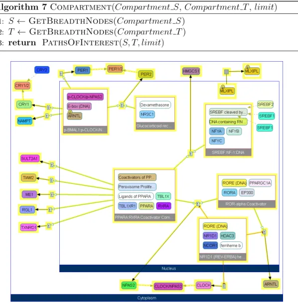
Compartment query can be seen as a special application of Paths Of Inter-est query, described in Algorithm 3, and this is reflected in its design (Algo-rithm 7). As a result, its time complexity is the same as Paths Of Interest, which is O(|V | + |E|). The query requires source compartments, target compartments, and a distance limit. The breadth nodes in source compartments are extracted to form the source set and the ones in target compartments form the target set. Then simply a Paths Of Interest query is performed using these sets in order to obtain the paths that originate in source compartments and terminate at target compartments, that are not longer than the specified distance limit.
Algorithm 7 Compartment(Compartment S, Compartment T , limit)
1: S ← GetBreadthNodes(Compartment S) 2: T ← GetBreadthNodes(Compartment T ) 3: return PathsOfInterest(S, T, limit)
As an example to compartment query, Figure 3.4 represents all the paths starting from nucleus and ending at cytoplasm, found in “Signaling by EGFR” model. The paths generally represent transcription regulation events taking place in nucleus, probably the end result of the cascade initiated by EGFR.
3.3
Path Iteration Query
There may be cases where a researcher has to deal with a huge and complex pathway view and may not have a specific set of proteins that can be used as a start point for decomposing such a huge graph. In that case, the previously described query algorithms will not be applicable as they all require an initial set of seed nodes. Considering such cases, another query has been designed, whose basic aim is to extract meaningful paths in a complicated graph.
Algorithm 8 PathIteration
1: R ← ∅
2: C ← ∅
3: for all breadth-node n do
4: C ← Updated-BFS({n} , ∅, fwd, ∞) 5: for all node c ∈ C do
6: R ← R ∪ {n, c, c.label(fwd)} 7: ResetLabel(C, fwd)
8: ResetColor(C)
9: sort R in order of decreasing labels
10: return R
The logic of this approach can be seen in Algorithm 8. In Line 4, we see that the algorithm performs a downwards breadth-first search starting from every single breadth node found in the pathway without a distance limit or target set. Then, a result set is formed, which contains the start node, the node that has been reached at the end of the search, and the distance between them. This means that the query finds the pairwise paths between the breadth nodes found in the graph. After this pair building step, resulting pairs are sorted in descending order of distances. The reason behind this sorting step is that the longer the path, the more information it will contain. The path obtained in this way will be long
(a) A complex graph and the dialog listing the paths found within this pathway
(b) The selected option is visualized with the path highlighted in yellow
enough to display enough information for a random starting point of analysis and short enough to yield a simpler network than the original one. The complexity of this algorithm is clearly O(|V | × (|V | + |E|)).
The actual result of the query is left to be decided by the user. A subset of sorted list of pairs are displayed to the user (Figure 3.5(a)). The dialog first lists all the paths with the longest distance. If their number is smaller than 10, then the paths are added in decreasing order of distance until the number reaches to 10. Then only the path selected by the user is visualized (Figure 3.5(b)).
3.4
Adapting Query Algorithms
The graph querying algorithms explained in Section 2.3 can be useful tools in analyzing biological pathways more deeply. Therefore, we have decided to imple-ment them in ChiBE in order to offer a wider range of queries. The important point to note here is that all queries will be making use of Updated-BFS given in Algorithm 6, instead of the regular breadth-first search detailed in Algorithm 1. With this simple adaptation, these query algorithms will become applicable to the biological pathways. Upcoming sections will explain why one might need to use these queries in context of a biological pathway and then give example results to demonstrate their implementations.
3.4.1
Neighborhood Query
In biological pathways, neighborhood of a protein contains valuable information related to that particular protein. From looking at the neighborhood, one can learn the molecules regulating that protein, the remaining substrates of the re-action that it is involved with or the proteins that are targeted by it. So we have decided to implement Algorithm 2 in order to identify the neighborhood of molecules of interest found in a pathway model.
this query, 1-level neighborhood of HEY1 entity has been searched. The resulting path is highlighted in yellow.
Figure 3.6: An example result for Neighborhood query
3.4.1.1 Entity vs State
At a given instance, a cell contains many different versions of a given molecule. In nucleus, it can be found as its gene as part of DNA. It can be translated into a protein and that protein may undergo different modifications, such as phosphorylation or cleavage. Although they have very different properties from each other, they still can be collected to form one type of biological molecule.
In BioPAX ontology [1], a distinction between these cases is applied. Each different version is called a state of that molecule. Entity is used to describe the collection of all states of a particular molecule. For instance, BRCA1 can be used to describe an entity without specifying a particular modification or cellular localization whereas phosphorylated BRCA1 is a state of BRCA1 entity.
While searching a given pathway model, breadth-first search can use either a specific state as part of the given set of molecules or can collectively use all of the states if an entity based search is preferred. Consider the query displayed in Figure 3.6. In that example an entity based search is requested, therefore all of the different versions of HEY1 entity is included in source set and the paths that
are reached from any of them is included in the result. However for performing the query seen in Figure 3.7, a specifically selected state of HEY1 is given as the source. As a result, the path that can only be reached through the particular state has been discovered at the end of the query.
Figure 3.7: An example result for state-based Neighborhood query
The choice between an entity-based and a state-based query can be made at the starting point of the query. When the menu item offered in top menu bar is used, user is required to specify entities for the query. There is also a pop-up menu that is reachable through each node in the pathway view and it can be used to specify a state-based query. Particular states of an entity that the user is interested in need to be selected on the pathway view, then a query that only uses these specified states is performed. With this distinction, users will be enabled to focus on specific version of a given molecule without obtaining results for unrelated states of an entity.
In the remaining of the query discussions, it will be assumed that entity-based version is used unless specified otherwise.
3.4.2
Paths From To Query
Biological interactions tend to be targeted pathways, starting at a specific molecule and ending at an effector molecule through intermediate pieces. Cas-cade of proteins can transfer a signal throughout the cell in order to complete a
cellular event. At certain situations, understanding the flow of these interactions may become critical or helpful. Therefore we have made use of Paths Of Interest query approach (Algorithm 3) to develop a query that will answer this need. To make the premise of query more clear to the user, we have called the query as “Paths From To”.
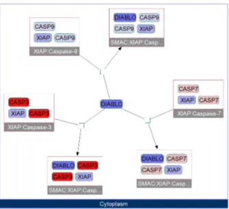
Figure 3.8 shows an example result. The source molecule is CASP9 and the target molecule is CASP3, length limit is 2. With these parameters, ChiBE returns the requested path in a new view with the result being highlighted. One point to note here is that Paths From To can only be performed in an entity-based manner. This is because one cannot distinguish between source nodes and target nodes when a simple selection on graph is used to specify the nodes of interest. As the distinction between source and target nodes is not available, we cannot offer a state-based query for this type.
Figure 3.8: An example result for Paths From To query
3.4.2.1 Alternative Types
In Algorithm 3, we have described a way of implementing Paths Of Interest query. However, there are also other versions of this query type offered in ChiBE, with slight modifications.
One of the changes concerns the determination of search distance limit. In the original implementation, user is expected to define a positive integer as the limit. However, there may be cases where the user does not have an idea about the size of the path. For these situations, we offer a shortest-path based distance limit. ChiBE first calculates the length of shortest path between the source and target nodes. Then as the distance limit, the summation of shortest path’s length and a user defined parameter limit is used. The changes that has been done can be seen in Algorithm 9. The length of shortest path is calculated by summing the forward and reverse distance labels of nodes in the candidate set (Line 5) as this will return the length of the path passing through a node. The minimum of these summations will give the minimum length of the path that can pass through any node in the network. With this new distance limit calculation approach, users can easily recover paths based on the shortest distance between the two sets. Like Paths Of Interest algorithm, this algorithm’s time complexity is O(|V | + |E|). Algorithm 9 PathsOfInterest-Shortest(S, T , limit)
1: C ← BFS(S, ∅, fwd, ∞) 2: ResetColor(C)
3: C ← C ∪ BFS(T, ∅, rev, ∞) 4: R ← ∅
5: shortest ← minimum(v.label(fwd) + v.label(rev)) where v ∈ C 6: for all node n ∈ C do
7: if n.label(fwd) + n.label(rev) ≤ shortest + limit then 8: R ← R ∪ {n}
9: return R
The second modification is about handling the relationships within source set and target set. Algorithm 10 shows its difference from Algoritm 3. Instead of calling breadth-first searches with empty target sets, this modified type defines a search with target sets. This means that the search stops at the first time a node from the target set is reached during traversal and as a result, the paths that start from a source (target) node and end at a source (target) node are not added to the result set. So this query strictly finds the paths from source nodes to target nodes and ignore relationships observed within sets.
Algorithm 10 PathsOfInterest-Strict(S, T , limit)
1: C ← BFS(S, T, fwd, limit) 2: ResetColor(C)
3: C ← C ∪ BFS(T, S, rev, limit) 4: R ← ∅
5: for all node n ∈ C do
6: if n.label(fwd) + n.label(rev) ≤ limit then 7: R ← R ∪ {n}
8: return R
3.4.3
Paths Between Query
Paths From To query focuses on paths that follows a particular direction, however there may be cases where a user is interested in all paths between a set of molecules rather than a subset of them in a specific direction. The cases where a researcher is interested in a number of proteins but does not know the true nature of the relationship between these molecules are suitable candidates for making use of this query. To provide a solution, we require a query type that finds the paths between the molecules in a single set, irrespective of path direction and Graph of Interest query explained in Algorithm 4 is the exact answer to this problem. In context of ChiBE, this query is called “Paths Between” again to be more clear about the nature of the query.
The sample pathway view seen in Figure 3.9 is the result of a Paths Between query, with NBN and MRE11A entities specified as the source set. The length limit in this case is 2.
Figure 3.9: An example result for Paths Between query
3.4.4
Common Stream Query
A single transcription factor can regulate the expression of multiple different proteins. Conversely, a single protein might be regulated through the action of multiple molecules. The general trend in these cases is that there may be common molecules in the upstream or downstream of a particular set of molecules. Discov-ering these common regulators or targets is an important step in understanding the causative relationships between these molecules. To be able to identify these paths, we have made use of Commons Stream query described in Algorithm 5.
Example result for this query type can be seen in Figure 3.10, in which the common downstream of TP53 and ATF2 with distance limit of 3 has been searched.
Figure 3.10: An example result for Common Stream query
3.5
Pathway Commons Queries
All of these queries described up to this point are performed on currently loaded model. This means that the search space is limited to the pathway model that has been loaded. ChiBE offers another set of queries with a much wider search space: Pathway Commons Database [9]. Instead of being limited to the model in hand, users can perform queries to this remote database. Another advantage is that users can use these queries to obtain a model to start working with when they do not have a model in hand.
Neighborhood, Paths Between, Paths From To, and Common Stream queries detailed in Section 2.3 are offered in this set. In local queries, input set of molecules is selected from the entities found in the model, whereas to perform Pathway Commons queries, HGNC symbols [26] of molecules need to be supplied. The remaining set of inputs for queries, such as direction and distance limit, are similar to their counterparts in local queries. Based on these given inputs and query type, ChiBE performs searches on the Pathway Commons database using
these query algorithms. The result is then presented to the user in a new view. There are two other query types that are performed on Pathway Commons database, but these are not available for local models. The first one is called Pathways With Keyword, which as its name suggests performs the query based on a given keyword. The keyword is searched in the database in order to extract the pathway models containing the given keyword. The list of pathways obtained through this search is presented to the user in a dialog. For instance when “EGFR signaling” is given as the keyword, the list of pathways seen in Figure 3.11 is obtained from Pathway Commons database. Then user simply needs to choose one of them for it to be retrieved from the database for visualization. This query is especially useful for the cases where user is interested in a topic but does not possess a BioPAX model related to it.
Figure 3.11: A sample result of Pathways With Keyword query
The second query specific to Pathway Commons is called Object With Database ID. This query asks for the RDF ID of an object of interest and then retrieves it from Pathway Commons database.
All of these different queries offers users an easy to use connection to Pathway Commons database. Normally one needs to search a database, download the
model from the database and then open that model in a tool. However thanks to these queries, users can perform all of these steps within ChiBE in one click which eases the process of reaching to a pathway view.
Chapter 4
High Throughput Data
Integration
Integrating high throughput experiment results, such as microarray or copy num-ber variation experiments, in an easy and understandable way is an important step in the analysis of these data in pathway context. This chapter will focus on the efforts related with the solutions offered by ChiBE to this problem. In the first section, microarray data integration through GEO database will be dis-cussed. Then the next section focuses on genomic data integration and the cBio Cancer Genomics Portal.
4.1
Fetch From GEO
ChiBE 1.0 offers users a flexible and comprehensive feature of integrating exper-iment results with pathway view. Expression, mass spectrometry, copy number variation and mutation data can be loaded onto the network after the user has manually performed a mapping between experiment results and entities in the pathway view. This manual step of mapping can be overwhelming and may put off users from utilizing this feature. Therefore, we decided to offer simpler alter-native with a smaller scope in order to eliminate the need for manual user input
![Figure 2.2: Different glyphs supported by ChiBE to represent different biological entities and relationships [35]](https://thumb-eu.123doks.com/thumbv2/9libnet/5833320.119478/26.918.208.752.762.1002/figure-different-supported-represent-different-biological-entities-relationships.webp)