IMPROVING THE PERFORMANCE OF
SIMILARITY JOINS USING GRAPHICS
PROCESSING UNIT
a thesis
submitted to the department of computer engineering
and the graduate school of engineering and science
of bilkent university
in partial fulfillment of the requirements
for the degree of
master of science
By
Zeynep Korkmaz
November, 2012
I certify that I have read this thesis and that in my opinion it is fully adequate, in scope and in quality, as a thesis for the degree of Master of Science.
Prof. Dr. Cevdet Aykanat (Advisor)
I certify that I have read this thesis and that in my opinion it is fully adequate, in scope and in quality, as a thesis for the degree of Master of Science.
Assoc. Prof. Dr. Hakan Ferhatosmano˘glu (Co-Advisor)
I certify that I have read this thesis and that in my opinion it is fully adequate, in scope and in quality, as a thesis for the degree of Master of Science.
Prof. Dr. ¨Ozg¨ur Ulusoy
I certify that I have read this thesis and that in my opinion it is fully adequate, in scope and in quality, as a thesis for the degree of Master of Science.
Assoc. Prof. Dr. O˘guz Ergin
Approved for the Graduate School of Engineering and Science:
Prof. Dr. Levent Onural Director of the Graduate School
ABSTRACT
IMPROVING THE PERFORMANCE OF SIMILARITY
JOINS USING GRAPHICS PROCESSING UNIT
Zeynep Korkmaz
M.S. in Computer Engineering
Supervisors: Prof. Dr. Cevdet Aykanat and Assoc. Prof. Dr. Hakan Ferhatosmano˘glu
November, 2012
The similarity join is an important operation in data mining and it is used in many applications from varying domains. A similarity join operator takes one or two sets of data points and outputs pairs of points whose distances in the data space is within a certain threshold value, ε. The baseline nested loop approach computes the distances between all pairs of objects. When considering large set of objects which yield too long query time for nested loop paradigm, accelerat-ing such operator becomes more important. The computaccelerat-ing capability of recent GPUs with the help of a general purpose parallel computing architecture (CUDA) has attracted many researches. With this motivation, we propose two similarity join algorithms for Graphics Processing Unit (GPU). To exploit the advantages of general purpose GPU computing, we first propose an improved nested loop join algorithm (GPU-INLJ) for the specific environment of GPU. Also we present a partitioning-based join algorithm (KMEANS-JOIN) that guarantees each parti-tion can be joined independently without missing any join pair. Our experiments demonstrate massive performance gains and the suitability of our algorithms for large datasets.
Keywords: Similarity join, k-means clustering, general purpose graphics process-ing unit, CUDA.
¨
OZET
BENZERL˙IK B˙IRLES
¸ ˙IMLER˙IN˙IN PERFORMANSININ
GRAF˙IK ˙IS
¸LEME B˙IR˙IM˙I KULLANILARAK
ARTTIRILMASI
Zeynep Korkmaz
Bilgisayar M¨uhendisli˘gi, Y¨uksek Lisans Tez Y¨oneticileri: Prof. Dr. Cevdet Aykanat ve
Do¸c. Dr. Hakan Ferhatosmano˘glu Kasım, 2012
Benzerlik birle¸simi, veri madencili˘ginin ¨onemli i¸slemlerindendir ve ¸ce¸sitli alanlar-dan bir¸cok uygulamada kullanılmaktadır. Bir benzerlik birle¸simi i¸sleci bir ya da iki veri noktası k¨umesi alır ve veri uzayında birbirleri arasındaki uzaklık belirli bir e¸sik de˘geri, ε, arasında olan veri noktası ikililerini ¸cıktı olarak verir. Baz alınan i¸c i¸ce ge¸cmi¸s d¨ong¨u algoritması b¨ut¨un veri nesneleri arası uzaklık hesabı yapar. ˙I¸c i¸ce ge¸cmi¸s d¨ong¨u algoritması i¸cin ¸cok fazla sorgu zamanı tutan, b¨uy¨uk veri k¨umeleri dikkate alındı˘gında, b¨oyle bir operasyonu hızlandırmak daha da ¨onemli olmak-tadır. G¨un¨um¨uz grafik i¸slemcilerinin, genel ama¸clı paralel hesaplama mimarisinin de (CUDA) katkısıyla, hesaplama kapasiteleri bir¸cok ara¸stırmaya ¨on ayak olmak-tadır. Bu motivasyonla, iki tane Grafik ˙I¸sleme Birimi (G˙IB) tabanlı benzer-lik birle¸simi algoritması ¨onermekteyiz. ˙Ilk olarak, genel ama¸clı G˙IB programla-manın avantajlarından faydalanmak i¸cin, G˙IB’in kendine ¨ozg¨u ¨ozelliklerine uy-gun olan, geli¸stirilmi¸s i¸c i¸ce ge¸cmi¸s d¨ong¨u algoritması (GPU-INLJ) ¨onermekteyiz. Ayrıca herhangi bir birle¸sim ikilisi kaybına yol a¸cmadan, her b¨ol¨um¨un birbirinden ba˘gımsız olarak benzerlik birle¸simini sa˘glamayı garanti eden, b¨ol¨umleme tabanlı benzerlik birle¸simi algoritması (KMEANS-JOIN) ¨onerilmektedir. Deneylerimiz b¨uy¨uk performans kazancı ve algoritmamızın b¨uy¨uk veri k¨umelerine uygunlu˘gunu g¨ostermektedir.
Anahtar s¨ozc¨ukler : Benzerlik birle¸simi, k-means k¨umeleme, genel ama¸clı grafik i¸sleme birimi, CUDA .
Acknowledgement
I would like to express my deepest gratitude to my supervisor Prof. Dr. Cevdet Aykanat and Assoc. Prof. Dr. Hakan Ferhatosmano˘glu for their guidance and encouragement throughout the development of this thesis. I would also like to thank Prof. Dr. ¨Ozg¨ur Ulusoy and Assoc. Prof. Dr. O˘guz Ergin for reviewing and commenting on this thesis.
I would like to thank to the Scientific and Technological Research Council of Turkey (T ¨UB˙ITAK) for providing financial assistance during my study.
My special thanks go to Mustafa Korkmaz, who contributed to the studies in this thesis.
I am grateful to my friends Seher and Enver for their moral support during my study. I am also grateful to my valuable friends Can, ˙Ilker, Salim and S¸¨ukr¨u for their kindness and encouragement. I also feel very lucky to have valuable friends, Seher, Gizem, Beng¨u, Elif and G¨ok¸cen who have always been with me.
Finally, I owe my deepest gratitude to my parents, Mendane and Mustafa Saka, and my husband Mustafa Korkmaz for their love and encouragement.
Contents
1 Introduction 1 1.1 Contribution . . . 2 1.2 Outline . . . 3 2 Background 4 2.1 Similarity Join . . . 4 2.2 K-means Clustering . . . 7 2.3 GPGPU Programming and CUDA . . . 83 Related Work 12
3.1 CPU based Similarity Join . . . 12 3.2 GPU based Similarity Join . . . 18 3.3 GPU based K-Means Clustering . . . 19
4 Solving Similarity Join Problem on GPU 20 4.1 Parallel Nested Loop Algorithm . . . 20
CONTENTS vii
4.2 Improved Parallel Nested Loop Algorithm . . . 22
4.3 Parallel Clustering Based Partitioning and Epsilon Window Algo-rithm . . . 26
4.3.1 Partitioning Data . . . 26
4.3.2 Epsilon Overlaps between Clusters . . . 28
4.3.3 Replicated Clusters . . . 29
4.3.4 Creating Sorted Array . . . 32
4.3.5 Epsilon Join in Replicated Clusters . . . 32
4.3.6 Avoiding the Redundant Distance Comparison . . . 33
4.4 Reclustering based Epsilon Join . . . 35
5 Evaluation 37 5.1 Implementation Details . . . 37
5.1.1 Challenges and Optimizations . . . 37
5.1.2 Dataset . . . 39
5.2 Experimental Results . . . 40
5.2.1 Dataset Size . . . 41
5.2.2 Epsilon (Join) Selectivity . . . 46
5.2.3 Number of Clusters (k) Selectivity . . . 52
5.2.4 Reclustering with Different Workloads . . . 54
List of Figures
2.1 (a) The Non-self Similarity Join. and (b) The Self Similarity Join.. 5 2.2 Memory Hierarchy in CUDA . . . 11
3.1 ε-kdB Tree Structure . . . 14 3.2 Level Files of MSJ . . . 15 3.3 (a) The ρ-split function: D-index. and (b) The modified ρ-split
function: eD-index . . . 17 3.4 Two dimensional two level directory example . . . 19
4.1 CUDA block and corresponding shared memory . . . 22 4.2 GPU-based improved parallel nested loop algorithm Steps (a) First
step (b) Second step (c) Third step (d)Final step . . . 24 4.3 Voronoi Diagram based partitions and corresponding cluster
cen-troids . . . 27 4.4 Epsilon overlaps over the hyperplane between clusters . . . 28 4.5 The data point p belongs to the cluster with centroid c2, however,
LIST OF FIGURES ix
4.6 Finding an upper bound for data replication . . . 30 4.7 RE-JOIN algorithm schema . . . 36
5.1 Representation of a dataset with 100K data points . . . 39 5.2 Variation of running time of CPU-NLJ, GPU-NLJ and GPU-INLJ
with increasing dataset size. ε: 0.5 . . . 42 5.3 Variation of running time of GPU-NLJ, GPU-INLJ and
KMEANS-JOIN with increasing dataset size. ε: 0.5 and k: 20 . . . 42 5.4 Effect of dataset size on running time of main components of
KMEANS-JOIN. ε: 0.5 and k: 20 . . . 43 5.5 Percentage contribution of main components of KMEANS-JOIN
algorithm in terms of running time. ε: 0.5 and k: 20 . . . 44 5.6 Effect of dataset size on running time of GPU-NLJ-join kernel,
GPU-INLJ-join kernel and KMJ-join kernel. ε: 0.5 and k: 20 . . 45 5.7 Total number of replicated data points and corresponding number
of join pairs for varying number of data size in KMEANS-JOIN algorithm. ε: 0.5 and k: 20 . . . 46 5.8 Effect of ε on running time of GPU-NLJ, GPU-INLJ and
KMEANS-JOIN, datasize: 100K and k: 20 . . . 47 5.9 Effect of ε and k on compared-pairs-ratio of KMEANS-JOIN,
datasize: 100K . . . 48 5.10 Total number of replicated data points and corresponding number
of join pairs for varying values of ε in KMEANS-JOIN algorithm. datasize: 100K clustered dataset and k: 20 . . . 49
LIST OF FIGURES x
5.11 Total number of replicated data points and corresponding number of join pairs of color moments dataset for varying values of ε in KMEANS-JOIN algorithm. k: 20 . . . 49 5.12 Effect of ε on running time of CPU-NLJ, GPU-NLJ, GPU-INLJ
and KMEANS-JOIN algorithms for color moments dataset . . . . 50 5.13 Total number of replicated data points and corresponding number
of join pairs for varying values of ε in KMEANS-JOIN algorithm. datasize: 100K uniform dataset and k: 20 . . . 51 5.14 Effect of ε on running time of CPU-NLJ, GPU-NLJ, GPU-INLJ
and KMEANS-JOIN algorithms for 100K uniform dataset . . . . 51 5.15 Effect of k on running time of KMEANS-JOIN algorithms . . . . 52 5.16 Effect of k on running time of APRX-KMEANS-JOIN algorithms
ε: 0.4 . . . 53 5.17 Effect of k on precision values of APRX-KMEANS-JOIN
List of Tables
5.1 Speedup of KMEANS-JOIN algorithm over CPU-NLJ, GPU-NLJ, and GPU-INLJ for varying dataset size . . . 44 5.2 Speedup of GPU-NLJ and GPU-INLJ over CPU-NLJ for varying
dataset size . . . 45 5.3 Running times (seconds) for Update Intensive RE-JOIN . . . 55 5.4 Running times (seconds) for Query Intensive RE-JOIN . . . 56
Chapter 1
Introduction
Effective retrieval of knowledge is an important issue in database systems. As a result of increase in the database size, a second requirement is the efficiency. Al-though the primary design goal of the GPUs is processing of the graphics, the chip level parallelism encourages the developers to carry out general purpose comput-ing on GPUs. Therefore, many research communities such as data management started to use the computational capabilities of GPUs for computationally in-tensive applications. The CUDA programming model, which is developed by NVIDIA [1], allows programmers write scalable parallel programs using abstrac-tions as extension of the C language for utilizing multi-threaded GPUs.
The similarity join is a basic and powerful database operation for similarity based analysis and data mining in which we are given a large set D of objects which are usually associated with a vector from a multidimensional feature space. A well known application of the similarity join is searching pairwise similar objects in datasets. The most common similarity join type is ε-join (distance range join) which takes an application defined ε threshold and the query outputs pairs of points whose distances are not larger than ε.
If we focus on the complexity of similarity join queries, the baseline nested loop algorithm for similarity join operator has a complexity of O(n2) where n is the number of data points in the data set D. Thus, accelerating similarity join
operator and exploiting the parallelism potential of it is crucial for performance improvements and applications that employs it. Our aim in this thesis is to provide faster ε-join queries for a high number of data objects. For this purpose, we use general purpose computing on GPUs and CUDA programming model.
1.1
Contribution
In this thesis, we aim to accelerate similarity join operation using GPU. Firstly, we focus on baseline nested loop join algorithm, where no indexes exist and no preprocessing is performed. Then we implement a communication scheme between CUDA blocks which uses shared memory as much as possible to gain more speed up. Achieving high performance gains in this improved parallel nested loop approach yields a motivation to use it in independent partitions of the data set for faster query time. The major contributions of this thesis are as follows:
• We first propose an efficient GPU implementation for the nested loop join. It differs from previously proposed approaches in using shared memory more efficiently and paying attention to the memory operations. The proposed com-munication scheme between CUDA blocks also satisfies the correctness of the join results.
• We propose another approach for similarity join which uses parallel k-means clustering algorithm to partition the data, and provide ε boundaries between clusters to guarantee obtaining the ε-join results properly. After acquiring in-dependent partitions, the join operation for these partitions can be handled by the improved parallel nested loop join algorithm proposed in this thesis. In this approach, each step of the algorithm; partitioning, calculating epsilon bounds, finding replicated points and finally join operation is implemented in GPU which provides faster and scalable performance results.
• One of the major problems in parallel join algorithms is the redundant or multiple join pairs. We propose a duplicate join pair removal technique which also eliminates the number of redundant distance comparison between data points.
This technique only requires bitwise operations which are performed very fast on GPU. It overcomes the problem of any pair appear in multiple clusters caused by replicating data points between clusters.
• Finally, we propose a solution for similarity join problem in a dynamic dataset which is updated by new data points iteratively. In this problem, new data points arrive and we keep them in a cluster based index. This cluster based index provides producing the join results faster when epsilon query is requested on the updated dataset.
1.2
Outline
The rest of this thesis is organized as follows. In Chapter 2, some background information for the proposed work; similarity join problem, k-means clustering algorithm and general purpose GPU programming is given. In Chapter 3, we mention about the previously proposed CPU- and GPU-based related works. In Chapter 4 we present our GPU-based solutions for similarity join problem using GPU. Then, we demonstrate our experimental evaluations in Chapter 5 and finally we conclude the thesis in Chapter 6.
Chapter 2
Background
In this section, first similarity join problem is defined; secondly k-means clustering algorithm and then a brief description of General Purpose Graphics Processor Unit (GPGPU) programming and Compute Unified Device Architecture (CUDA) are given.
2.1
Similarity Join
The similarity join is a basic operation for similarity based analytic and data mining on feature vectors. In such applications, we are given one (D) or two large sets (S and D) of objects which are associated with a vector from a mul-tidimensional space, the feature space. In similarity join, pairs of objects must satisfy a join condition on (D × D) or (D × S). In general, join condition provide the similarity between objects in metric spaces, especially in Euclidean distance. The most common similarity join operator type is the ε-join which is also called as distance range join. The scope of this thesis is restricted to the distance range join and we will use similarity join and ε-join instead of distance range join. There are two versions of the similarity join problem, which are self join and non-self join.
(a) (b)
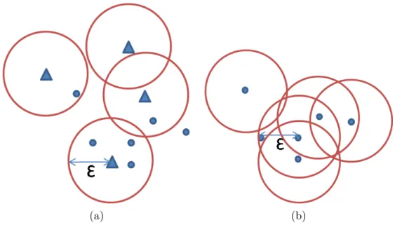
Figure 2.1: (a) The Non-self Similarity Join. and (b) The Self Similarity Join..
In Figure 2.1-a, the small circles represent the points of set D and the triangles represent the points of S. It visualizes the non-self ε-join query. The formal definition is given below:
Definition 1: For two data sets S and D; let S and D be sets of feature vectors of a d-dimensional vector space and ε ∈ R+ be a given threshold. Then the non-self similarity join consists of all pairs:
(p ∈ S, q ∈ D)| q
(p − q)T(p − q) ≤ ε
In Figure 2.1-b, the circles represent the points of set D, and visualizes the self-ε-join query. The formal definition is given below:
Definition 2: For a data set D; let D be a set of feature vectors of a d-dimensional vector space and ε ∈ R+ be a given threshold. Then the self simi-larity join consists of all pairs:
(p, q) ∈ (D × D)| q
The baseline solution for the similarity join algorithm is the nested loop paradigm. The nested loop join iterates each object of set D in the outer loop and in the inner loop, each object from D scans the each object from S by calculating the distance and comparing it with ε threshold. If it is self similarity join query, than the inner loop also contains the objects from the set D. The pseudo code for nested loop similarity join is given in Algorithm 1.
Algorithm 1 The Nested Loop Similarity Join Algorithm
1: for all p ∈ D do 2: for all q ∈ S do 3: if dist(p, q) ≤ ε then 4: (p, q) is a result pair 5: end if 6: end for 7: end for
Another solution for the similarity join algorithm is the indexed nested loop join. In this solution, in the outer loop, the objects of set D iterates over a index structure on the objects of set S. The nested loop join can be improved by replacing the inner loop with a multidimensional index structure. From the ε-join point of view, the index structure in the inner loop provides a range in which the outer loop objects scan over. The pseudo code for indexed nested loop similarity join is given in Algorithm 2.
Algorithm 2 The Indexed Nested Loop Similarity Join Algorithm
1: for all p ∈ D do
2: range ← index(p, D, ε)
3: for all q ∈ range do
4: if dist(p, q) ≤ ε then
5: (p, q) is a result pair
6: end if
7: end for
The more sophisticated solutions for similarity join problem will be introduced in the Chapter 3.
2.2
K-means Clustering
The k-means algorithm [2] [3] is a well known and widely used clustering method. It assigns each data point to the closest cluster by looking at the distances between data points and centroids of the clusters. The centroid of a cluster is defined as the mean position of the data points in that cluster. More formal definition is given below.
Definition 3: Let D ⊆ Rd be a set of data points (D
1...n) of a d-dimensional
vector space, the clustering is to partition the n data points into k clusters (P1...k)
with centroids C1...k, where k ≤ n in order to minimize the sum of squares of
distances of each cluster.
minPk
i=1
P
Dj∈Pi(kDj− Cik)
2
The standard k-means algorithm [3] is a heuristic solution for an NP-hard problem in Euclidean space. As shown in Algorithm 3, there are two main steps in each iteration. First one is the updating cluster centroids which computes the mean from assigned objects of each cluster. Second one is the labelling of data points which assigns each data object to its closest cluster by computing the distance between cluster centroids. The algorithm terminates when the centroids no longer move.
Algorithm 3 The Standard k-Means Algorithm
1: Select k data points as initial centroids
2: repeat
3: Assign each data point to the cluster of closest centroid 4: Recompute the means of clusters and update centroids
In this thesis, we take the grouping advantage of k-means algorithm that data points within one cluster have similar characteristic. However, in each iteration of k-means algorithm, the labelling step, which calculates the distance between data points and new cluster centroids dominates the computation time and it is very costly. Since the labelling step for each data points is independent of each other, it can be performed in parallel. Parallelizing k-means algorithm or square error clustering has also proposed in order to overcome this costly computation requirement and considerable speed-ups were reported previously [4] [5]. Improving the performance of k-means clustering algorithm can be achieved by using GPU computing. Existing GPU-based k-means algorithms [6] [7] are given in Section 3.3. In this study, we also need a fast clustering algorithm and use GPU for performance improvement in clustering. We use the software which includes CUDA based implementation of k-means clustering algorithm under the open-source MIT licence [8].
In this thesis, we use k-means clustering algorithm to partition data into sets of points that are close to each other and use its property that the partitions represent the Voronoi cells generated by the means and data is split halfway between cluster means [9].
2.3
GPGPU Programming and CUDA
Recent improvements in the performance of GPUs is increasing with parallelism. The growth of processor performance and hardware parallelism show that the modern GPUs are suitable for the needs of a problem with tremendous paral-lelism and effectively solve general purpose computational problems, which is called as general purpose computation on graphics processors (GPGPU). Run-ning the parallel algorithms on GPUs provides massive speedups over similar CPU algorithms.
NVIDIA developed CUDA [1], a general purpose parallel computing archi-tecture with a parallel programming model for NVIDIA GPUs with hundreds of
cores. This programming model provides developing scalable parallel programs by using some extensions to C programming language. It also helps to solve complex computational problems efficiently. This innovative architecture increase the per-formance and ability of GPGPU. In CUDA programming model, there are some important extensions of C programming language to express parallelism which are hierarchy of thread groups, shared memories and barrier synchronization.
In CUDA, there are some terms that are important to understand the pro-gramming model. These are host, device and kernel.
• Host: Host in CUDA includes CPU and RAM. Codes written in host is same as standard C programming language and generally are used for some initializations and transferring data between GPU and CPU.
• Device: Device in CUDA refers to GPU environment which includes GPU and GPU memory. Parallel executions of program are run in device. Its is completely different than CPU environment and many challenges need to be overcome.
• Kernel Function: Kernel in CUDA refers to functions that run in CUDA threads. Kernel is a C function which is executed in multiple CUDA threads multiple times and all threads use the same kernel function. A kernel can be defined using the global identifier and the thread organization of the execution can be written in function call in <<< and >>> as block grid dimension and thread block dimension.
In CUDA programming model, there are also some parallel programming structures which are thread hierarchy and memory hierarchy.
• Thread Hierarchy: CUDA executes the threads as thread blocks, which refers to a structure including a certain number of threads that are executed concurrently. As a result of block size restrictions, CUDA executes thread blocks in grids. A grid organization decides how many times the kernel will be executed as blocks. A grid can be identified as 1, 2 and 3 dimensional blocks. In CUDA programming model, current thread and block can be identified by using the
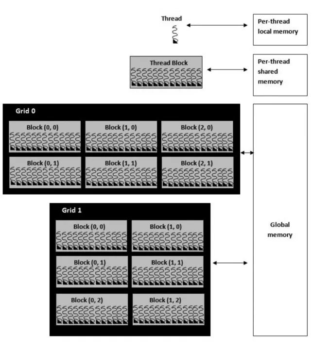
built-in variables which are threadIdx and blockIdx respectively. As a result of CUDA thread hierarchy, iterative executions are different than traditional loops. • Memory Hierarchy: We demonstrate the three most common memory types in CUDA which are global memory and shared memory. An illustration of memory types is shown in Figure 2.2 [1].
Global memory is the main memory of the device because it is also visible from the host and its lifetime is same with an application. The data that we need to use, is transferred from the host to global memory. It is also visible to all threads regardless of their grid or block information. However, it is relatively much slower than other CUDA memory types like shared memory and it is not cached. A variable which declared only with device qualifier, resides in global memory space.
Shared Memory has the life time of its corresponding block and is only accessi-ble from all the threads in that block. A variaaccessi-ble which declared with shared qualifier, resides in shared memory space of a thread block. Its space is quite little, however, it is much more faster than global memory. This trade-off is the main struggle in CUDA. Most of the speed optimization is bounded up to shared memory usage.
Another type of memory is local memory. Every thread uses implicitly its local memory. Thus, its life time is related with its thread.
Chapter 3
Related Work
Join queries are major parts of many data mining algorithms, and they are also very time consuming because of high complexity. For this purpose, many re-searches have been addressed to increase the performance of join algorithms. In Section 2.1, nested loop and indexed nested loop paradigms are introduced. This chapter includes more sophisticated algorithms and the scope of these algorithms varies from spatial joins to similarity joins. There are many index structures that have been employed for join processing, such as R-Trees [10], Seeded Trees [11], and ε-kdb Trees [12]. There are also some partitioning methods [13] [14] which require data point replication. Also there exists join algorithms based on metric space indexing method [15] and join algorithms based on sorting [16] [17].
3.1
CPU based Similarity Join
In this section, we explain some of the previously proposed CPU based algorithms related to join queries.
Efficient Processing of Spatial Joins Using R-Trees: Spatial joins ba-sically combine two or more datasets based on their spatial relationship. Spatial joins consist of two main steps which are filter and refinement steps. In the filter
step, tuples that cannot belong to the result set are eliminated. In the refinement step, possible results decided in the filter step are checked if they belong to the result set. Spatial joins, especially the refinement steps, are expensive operations and efficiently performing them has attracted many researchers. There are some spatial index structures such as R-trees [18], and it is used to improve the perfor-mance of spatial joins. Brinkhoff et al. [10] proposed a join algorithm on R-trees. This algorithm requires R-tree index on join inputs and performs a synchronized depth-first search of indices.
Seeded Tree: Lo and Ravishankar proposed an approach to perform spatial joins using seeded trees [11]. In spatial databases, there can be some situations where the inputs are intermediate results of a complex query, thus the join inputs do not have a spatial index on them. In this technique, the indices are not required on the inputs. It dynamically constructs index trees at join time. Seeded trees are R-tree like structures but they are allowed to be height unbalanced. In this technique, large number of random disk accesses during tree construction take the place of smaller numbers of sequential disk accesses.
Partition Based Spatial Merge Join: Patel and DeWitt proposed PBSM method for performing spatial join operation [14]. The algorithm first divides the input into manageable partitions and joins those partitions by using plane-sweeping technique. One of the beneficial contributions of PBSM algorithm is that it does not require indices on both inputs. The PBSM is a generalization of sort merge join. The algorithm first compute the number of partitions and these partitions act as buckets in hash joins and they are filled with corresponding entities.Then it joins all pairs of corresponding partitions and sorts the pairs and eliminates the duplicates. The data space in this approach is partitioned regularly and multiple assignment is needed for both input sets.
Spatial Hash-Joins: In this study, Lo and Ravishankar applied hash-join paradigm to spatial joins [13]. In this approach, first the number of partitions (buckets) are computed and the first input set is sampled to initialize the parti-tions. Then the buckets for second input set are partitioned using the buckets of first input set. Then the assignment function map the objects into multiple
buckets, if necessary. Finally the corresponding buckets are joined to produce the result. The data space in this approach is partitioned irregularly and multiple assignment is needed only for one dataset.
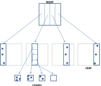
ε-kdB Tree: ε-kdB Tree is an indexing structure for the multidimensional join problem and proposed by Shim et al. [12]. This structure partitions the data space into grids and the join pairs of a point is found in the neighbouring cells. However, when considering the high number of dimensions, those neighbour grid cells increases to 3d− 1. ε-kdB Tree uses only a part of dimension to partition
rather than considering the cells one by one. This reduces the number of neigh-bouring cells that are considered for the join operation. Constructing ε-kdB Tree starts with a single leaf node and pointers to the data points are stored in the leaf nodes. It is assumed that the coordinates of the points in each dimension lie between 0 and +1. When the number of points in a leaf node exceeds the threshold, the leaf node is split and becomes an interior node. If the leaf node is at ith level, the ith dimension is used for splitting and the node is split into
b1/εc parts. Figure 3.1 [12], shows an example of ε-kdB Tree structure for two dimensional space.
Multidimensional Spatial Joins (MSJ): Koudas and Sevcik proposed Size Seperational Spatial Join algorithm (S3J ) [16] which uses hierarchical
decompo-sition for the data space and does not require replication of input sets as done in [14] and [13]. This algorithm uses space filling curves to order the points in multidimensional space. MSJ [17] is a generalization of Size Seperational Spatial Join algorithm [16]. Given two d-dimensional datasets, and ε distance predicate, the algorithm scan each data set and divide them into level files. Figure 3.2 visu-alize the level files. For doing this, the Hilbert values of the level files where the hypercubes(data points) belong are transformed. Then the level files are sorted into non-decreasing order of Hilbert values. Finally the merge phase of the par-titions is performed. This approach has scalability problems with the increasing dimensionality.
Figure 3.2: Level Files of MSJ
Generic External Space Sweep (GESS): Dittrich and Seeger proposed Generic External Space Sweep (GESS) et al. [19]. GESS reduces the number of expensive distance computations by using a replication algorithm. Each fea-ture vector is transformed into a hypercube with side length ε. The proposed replication algorithm creates codes for the representation of subspaces of each hypercube. GESS does not require partitioning the hypercubes into level files as done in [17], because it employs a sorting operator which applies lexicographic ordering on the hypercubes. Finally the Orenstein’s Merge Algorithm [20] is used
for the join phase.
Epsilon Grid Order (EGO): Epsilon Grid Order [21] was proposed for solving the similarity join problem of very large datasets. It tries to solve the scalability problem which is an important issue in grid based approaches such as Multidimensional Spatial Joins [17] and ε-kdB Tree [12]. EGO uses an external sorting algorithm and a scheduling strategy during the join phase rather than keeping the large amount of data in the main memory. The sort order is obtained by laying an equidistance grid with cell length ε over the data space and then comparing the grid cells lexicographically [21]. The EGO solve the problem of IO scheduling when the ε intervals of some points do not fit in the main mem-ory by proposing crab stepping heuristic. This heuristic minimizes the reads of neighbouring cells.
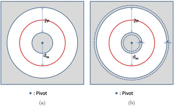
Similarity Join in Metric Spaces Using eD-Index: Previously, some techniques based on metric space indexing was also used for similarity joins. Dohnal et al. [15] proposed a metric space index called eD-index for self similarity join problem. The eD-Index is an extension of the D-Index [22] structure. The D-Index partitioning uses multiple ρ-split function [23] around separate pivots. It partitions the set into three subsets using the parameter ρ, the medium distance dm, and the pivot, as shown in Figure 3.3-a [15]. In Figure 3.3-a, the inner and
outer shaded areas contain the objects that their distance to pivot are less than or equal to dm − ρ and greater than dm+ ρ respectively. These sets are called
separable sets and the all others form the exclusion set. The eD-Index extends the D-Index by modifying the ρ-split function so that the separable and exclusion sets overlap of the distance ε. The objects which belong to both separable and exclusion sets shown in Figure 3.3-b [15] within the dotted lines, are replicated to prevent missing join pairs.
(a) (b)
Figure 3.3: (a) The ρ-split function: D-index. and (b) The modified ρ-split function: eD-index
The Quickjoin Algorithm: Jacox et al. [24] proposed a method for dis-tance based similarity join problem called Quickjoin which is conceptually similar to the Quicksort [25] algorithm. The Quickjoin partition the data into subsets recursively until they are small enough to be efficiently processed by using nested loop join algorithm and it provides windows around the boundaries of partitions. Also, the hyperplane partitioning [26], and the ball partitioning which partitions the data based on their distance to a random object are used to partition the data. The main difference between the Quickjoin and eD-Index [15] is that the Quickjoin creates subsets of ε regions which are processed separately, however, the eD-Index extends the partitions by ε.
List of Twin Clusters: Paredes and Reyes proposed List of Twin Clusters (LTC) [27], which is a metric index to solve similarity join problem and indexes both input sets jointly. LTC is based on List of Clusters (LC) [28], but uses clusters with fixed radius. The data structure in LTC considers two list of over-lapping clusters. Thus the twin cluster of range query object would contain the most relevant and candidate objects.
3.2
GPU based Similarity Join
The performance benefit of GPGPU technology has been recently used in database management problems [29] [30]. In [31], the authors present a GPU based relational query processor for main memory databases. Also, the sort op-eration which is important for query processing is improved using GPU [32]. Re-cently, the performance of well-known multidimensional index structure R-Tree has been improved by using GPU [33] [34].
There are a few study related to join queries on GPU. In [35], some data parallel primitives are demonstrated and these primitives are used to implement relational join algorithms such as sort-merge and hash joins with and without index support. In [36] and [37], which are most related studies to ours, the similarity join algorithm on GPU is examined.
LSS: A GPU-Based Similarity Join: In [37], a similarity join algorithm called LSS is proposed. LSS requires sort and search routines and it is based on the concept of space filling curves for pruning the search space. Basically LSS builds multiple space filling curves over one of the input sets and reduces the size of interval searches which are performed for the data points of other input set. LSS utilizes a GPU-based bitonic sort [38] algorithm to determine the z-order of objects.
Index Supported Similarity Join on Graphics Processor: In [36], a GPU-based parallelization of nested loop join (NLJ), and an indexed join algo-rithm are proposed. Parallelization of NLJ is performed by creating a thread which is actually the current query point, for each iteration of the outer loop and each thread is responsible for the distance calculations and comparison with ε threshold. This algorithm [36] and an our proposed improvements on it, espe-cially paying attention to the GPU specifications and proposed communication scheme between CUDA blocks are also mentioned in Section 4.1.
Figure 3.4: Two dimensional two level directory example
Another algorithm which provides an index structure to support similarity join on GPU (NLJ with index support) is also given in [36], [39]. In this algorithm, similar to the parallel NLJ, each individual thread traverses the index structure for inner loop in parallel. For the index structure, the data is partitioned according to the dimensions. For example, as shown in Figure 3.4 [36], in a two level directory, first level partitions the data over the first dimension and the second level partitions the data over the second level.
3.3
GPU based K-Means Clustering
Clustering is one of the most important data mining method which is widely used in many different areas. K-Means is one of the most famous and easy to implement clustering algorithm, however, it has performance disadvantages in large datasets. Therefore, improving the performance of k-Means is highly important in order to overcome computational requirement of many applications that use k-Means. Some recent works [40] [41] [6] [7] study performing k-Means clustering algorithm efficiently on GPU and important speedups were reported. In [6], a hybrid approach which parallelizes distance calculations on GPU and sequentially updates the cluster centroids is proposed. A CUDA based k-Means algorithm is also proposed in [7] and differs from previous approaches by utilizing triangle inequality to avoid unnecessary distance calculations.
Chapter 4
Solving Similarity Join Problem
on GPU
In this chapter, we describe our solutions for improving the performance of sim-ilarity join algorithm. Comparing the results of each approach is given and dis-cussed in Chapter 5. In Section 4.1, the GPU based parallelization of nested loop algorithm for similarity join (NLJ) which is proposed in [36], is explained. Then, we present our contribution and improvements over NLJ in Section 4.2. Finally, we propose clustering and reclustering based join algorithms in Section 4.3 and in Section 4.4 respectively.
4.1
Parallel Nested Loop Algorithm
The Nested Loop Similarity Join algorithm is highly parallelizable and its poten-tial for performance improvement is promising. High computing capabilities of recent GPUs is beneficial in order to explore this parallelizm and produce consid-erable improvements. In [36], a GPU-based parallel nested loop join algorithm is presented and In this section, we mention about this baseline algorithm. The pseudo code for the parallel nested loop similarity join algorithm (GPU-NLJ) is given in Algorithm 4.
Algorithm 4 GPU-NLJ
1: Input: S ∈ Rd, ε
2: q ← currentData[d]
3: shared sharedMem[d × NTHREADS]
4: globalIndex ← threadIdx.x + blockDim.x × blockIdx.x
5: localIndex ← threadIdx.x 6: q ← data[ globalIndex × d ] 7: for i = globalIndex + 1 to |S| do 8: synchronize threads 9: p ← sharedMem[localIndex × d] ← data[ i × d ] 10: if dist(p, q) ≤ ε then 11: count ← atomicInc(1) 12: synchronize threads
13: results[count] ← (p, q) {(p,q) is a result pair}
14: end if
15: end for
As shown in Algorithm 1, the inner loop operations are independent of each other and can be performed in parallel. In Algorithm 4, to parallelize NLJ algo-rithm by using GPU, first a thread which corresponds the current query point, is created for each iteration of the outer loop. Thus each thread takes the responsi-bility of the inner loop which performs the distance calculation and comparison in parallel. We avoid duplicate pairs by starting the inner loop index from the index of current query point. We use atomic operations [1] provided by CUDA to store the join pairs into the results array and avoid race condition, which oc-curs when threads share a common resource. The atomicInc operation overcomes this problem and provides incrementing the address of result array counter for concurrent writings to satisfy correct addresses for the result pairs.
4.2
Improved Parallel Nested Loop Algorithm
In Section 4.1, we explain the GPU-based parallel NLJ algorithm and we will report in Chapter 5 that it has significant performance improvement over NLJ algorithm on CPU (CPU-NLJ). However, it does not exploit the computing po-tential of GPU efficiently. Previously proposed GPU based similarity join studies [37] [36] tries to prune the search space of each data point belongs to the outer loop. In this study, first we aim to exploit the parallelism potential of NLJ algo-rithm on GPU. For this purpose, we propose a communication scheme between CUDA blocks which provides usage of shared memory as much as possible and compare the distance between Si and Sj data points only once where i 6= j and
S ∈ Rd to gain more speedup.
Before starting explaining our proposed improved NLJ (GPU-INLJ) algo-rithm, the importance of shared memory usage should be mentioned. Each CUDA thread block has its shared memory and the lifetime of shared memory is same as its corresponding thread block. Major problem of shared memory is its capac-ity (48KB). However, it is much faster than global memory. Thus the usage of shared memory is crucial for high performance. In fact most of the speed opti-mization is bounded up to shared memory usage. The trade-off between space and performance is the main struggle in CUDA programming.
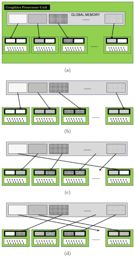
To better explain the GPU-INLJ algorithm, Figure 4.1 shows a CUDA block, threads in it and its corresponding shared memory. In Figure 4.2, this illustration is used to explain the steps of proposed algorithm.
At the beginning of the computation, the data is divided into a number of threads per block sized chunks and these chunks are distributed to the corre-sponding blocks. These chunks are only half size of the reserved shared memory per block, since other chunks will later reside on the other half of the shared memory. As an illustration, in Figure 4.2-a, an example of blocks of data is given.
Figure 4.2-b shows the first step in which each block copies itself to its cor-responding second half of the shared memory. Different from the next steps, in this step, each thread compares the corresponding data point (current) with the data points whose indexes are greater than the index of current data point. This step achieves to avoid idle comparison especially in diagonals.
Figure 4.2-c shows the second step. In this step, each block copies the data chunk in global memory which is mapped to the next block in modular fashion. Then each thread compares the corresponding data point in first half of the shared memory with all the data points in the second half of the shared memory.
Figure 4.2-d shows the final step. As in the previous step, each block copies the data chunk in global memory which is mapped to the next block of its next. To formulate the algorithm, (numberof blocks + 1)/2 steps are performed to guarantee that all pairs are compared. For iteration i, we copy the ((n + i)mod(numberof blocks))th chunk to the nth block then each thread in a block
compares the corresponding data point in the first half with each data point in second half of the shared memory.
(a)
(b)
(c)
(d)
Figure 4.2: GPU-based improved parallel nested loop algorithm Steps (a) First step (b) Second step (c) Third step (d)Final step
Algorithm 5 GPU-INLJ
1: Input: S ∈ Rd, ε
2: shared sharedMem[2 × NTHREADS][d]
3: globalIndex ← threadIdx.x + blockDim.x × blockIdx.x
4: localIndex ← threadIdx.x
5: NBLOCKS ← gridDim.x
6: sharedMem[localIndex] ← S[ globalIndex × d ]
7: synchronize threads
8: for i=0 to NBLOCKS / 2 do
9: index ← (blockIdx.x + i) × NBLOCKS
10: index ← (index × blockDim.x) × d + (threadIdx.x × d)
11: sharedMem[localIndex + NTHREADS] ← S[index]
12: synchronize threads
13: if i = 0 then
14: for j= localIndex+1 to NTHREADS do
15: q ← sharedMem[j + NTHREADS]
16: p ← sharedMem[localIndex]
17: if dist(p, q) ≤ ε then
18: count ← atomicInc(1)
19: results[count] ← (p, q) {(p,q) is a result pair}
20: end if 21: end for 22: else 23: for j= 0 to NTHREADS do 24: q ← sharedMem[j + NTHREADS] 25: p ← sharedMem[localIndex] 26: if dist(p, q) ≤ ε then 27: count ← atomicInc(1)
28: results[count] ← (p, q) {(p,q) is a result pair}
29: end if
30: end for 31: end if
4.3
Parallel Clustering Based Partitioning and
Epsilon Window Algorithm
In this section, we introduce parallel clustering based partitioning and epsilon win-dow algorithm (KMEANS-JOIN) for similarity join problem. In Section 4.2, we propose GPU-INLJ algorithm which provide a new communication scheme be-tween CUDA blocks via shared memory to improve the GPU-NLJ algorithm and achieve considerable speedups over it. With this motivation, we come up with a solution that partitions the data and replicate the data points into ε-boundaries of clusters to satisfy storing points into same partition which lie within ε distance of each other. Finally each independent partitions employ the GPU-INLJ algorithm to result join pairs. Algorithm 6 shows the major components of KMEANS-JOIN algorithm. KMJ-clustering is a GPU based k-Means Clustering algorithm. KMJ-epsilon-bound is a GPU kernel function which finds the data points that need to be replicated and clusters to which the data points are replicated. KMJ-sorted-array creates an array sorted by cluster id including the replicated data points, and finally KMJ-join-kernel is a GPU kernel function which performs the similarity join operation for each independent partition.
Algorithm 6 KMEANS-JOIN
1: Input: S[s1, s2, ..., s|S|] ∈ Rd, ε, k
2: centroids: C[c1...ck] and membership: M [|S|] ← KMJ-clustering(S, d, k)
3: overlapped data points: O ← KMJ-epsilon-bound (S, C, M)
4: count ← count-replicated-points(O)
5: sorted − S[(s1)c1...(sn)c1, ..., (s1)ck...(sm)ck] ← KMJ-sorted-array(S, O, M,
count)
6: KMJ-join-kernel(sorted-S, ε, k)
4.3.1
Partitioning Data
For our similarity join algorithm, first we need to divide the data into partitions to reduce the join cost. In the partitioning step which is called KMJ-clustering,
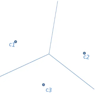
the main purpose is to cluster data points so that the points in the same partition are more likely to be joined according to the predefined threshold value ε. Thus we need to consider closeness of the data points while partitioning. Another important issue is the efficiency that requires a fast partitioning approach. For this purpose, we choose the k-Means clustering algorithm which converges very fast and can be parallelized by using GPU. Also the k-Means clustering algorithm provides partitioning the data space into Voronoi cells [9] which is explained in Section 2.2. For k-Means clustering implementation, we use the software which includes CUDA based implementation of k-means clustering algorithm under the open-source MIT licence and provided in [8]. It takes S[s1, s2, ..., s|S|] ∈ Rddataset
and number of clusters k as inputs and outputs the cluster centroids C[c1...ck]
and an array M [|S|] which stores the cluster index of each data point belongs. As shown in Figure 4.3, the partitions represent the Voronoi cells generated by the means and data is split halfway between cluster means. In Figure 4.3, c1,
c2 and c3 are the cluster centroids.
4.3.2
Epsilon Overlaps between Clusters
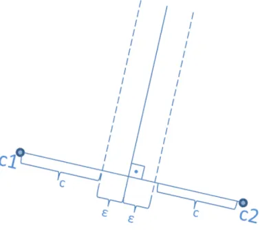
In the proposed KMEANS-JOIN algorithm, the final clusters of data will be considered as independent partitions and sent to KMJ-join-kernel which employs GPU-INLJ algorithm separately from each others without any communication requirements. Since the main aim is to perform ε-join operation, only clustering the data cannot guarantee the proper join results. For example, there can be objects that are close to each other in ε distance, but assigned to different clusters and this may cause missing join results. For this purpose, we suggest ε-overlaps between cluster boundaries. To visualize this approach, in Figure 4.4, we extend ε-overlaps over the hyperplane which is at equal distance between cluster centroids c1 and c2. Suppose that the distance between cluster centroids: |c1, c2| = 2c + 2ε.
In Section 4.3.3, we will explain how the data points are replicated to other clusters.
4.3.3
Replicated Clusters
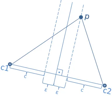
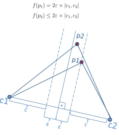
After clustering the data and divide it into separate partitions, we need to extend the hyperplane by ε and determine the data points that belong to a cluster but also need to be replicated to others whose ε-boundary also contains them. For this purpose, we need to determine an upper bound U B(p) for the data point p in Figure 4.5 which belongs to cluster with centroids c2 and lies within the ε-bounds
of cluster with centroids c1 as explained in Section 4.3.2.
Figure 4.5: The data point p belongs to the cluster with centroid c2, however, it
lies on the ε-bound line.
To determine an upper bound, for a point p which belongs to cluster c2, we
define a function as follows:
∀p ∈ c2, f (p) = |p, c1|2− |p, c2|2 (4.1)
We follow the findings in [42], we derive the Equation 4.2 for ε boundaries:
The right hand side of Equation 4.2 forms an upper bound for the functional values of points that lie within the ε boundary of c2 with respect to c1.
As shown in Figure 4.6, if a point is on the edge, then the functional value of it is equal to the upper bound, otherwise the inequality is strict. The functional values of points p1 and p1 which belong to c2 in Figure 4.5 are as follows:
f (p1) = 2ε × |c1, c2| (4.3)
f (p2) ≤ 2ε × |c1, c2| (4.4)
Figure 4.6: Finding an upper bound for data replication
For data point replication, we only need to know the distances between the cluster centroids, and the distances between each point and the cluster centroids. Thus, the replication process of each data point is independent from each other and the replicated clusters can be determined in parallel.
Using the observations in Equation 4.2, we come up with a replication scheme which checks if any point s belongs to cineeds to be replicated to cj by calculating
if the difference of the square of its distance to cj and ci is less than or equal to
s ∈ ci and s is replicated to cj, if f (s) ≤ U B(ci, cj)
Algorithm 7 explains the data replication and ε-bound algorithms. Algorithm 7 KMJ-epsilon-bound
1: Input: S ∈ Rd, ε, k, M, O, C
2: p ← currentData[d]
3: globalIndex ← threadIdx.x + blockDim.x × blockIdx.x
4: localIndex ← threadIdx.x
5: if globalIndex < |S| then
6: p ← S[globalIndex × d]
7: pc ← M[globalIndex]
8: for i=0 to k do
9: compute upper bound UB(p)
10: a ← dist(p, pc)
11: b ← dist(p, Ci)
12: if b2− a2 ≤ U B(p) then
13: report into O that p is replicated to Ci
14: end if
15: end for
16: end if
KMEANS-JOIN algorithm supports maximum 64 clusters. In Algorithm 7, we store the replicated points in a one dimensional and |S| size overlapping array (O) which allocates long integer types. Thus, each element in O represents a data point and keeps 64 bits. For a data point, we set its bits which represent the cluster id where that data point is replicated to. If we consider an 8 clusters example, assume that the ith data point is replicated to the 0th, 3th and 7th
clusters. In this case O[i] stores 10001001. We will use this storage schema in creating an array sorted (KMJ-sorted-array) by cluster id including the overlapped data points and reducing the redundant distance comparison which also eliminates the duplicate join pairs.
4.3.4
Creating Sorted Array
After finding the data points that need to be replicated and the clusters which the data points are replicated to, we create an array stores data points both original and replicated ones which are sorted (KMJ-sorted-array) by cluster id. As shown in Algorithm 8, we find the clusters where points are replicated to by pro-cessing the overlapping array O which is obtained as described in Section 4.3.3. In this step we obtain the final replicated clusters which will be handled indepen-dently by KMJ-join-kernel.
Algorithm 8 KMJ-sorted-array
1: Input: S[s1, s2, ..., s|S|] ∈ Rd, O, M, k
2: for i=0 to k do
3: store s into sorted − S if it belongs to cluster k, and increment index
4: for j=0 to |S| do
5: overlap ← O[j]
6: if overlap mod 2 = 1 then
7: sorted − S[index] ← sj 8: increment index 9: end if 10: overlap ← overlap / 2 11: O[j] ← overlap 12: end for 13: end for
4.3.5
Epsilon Join in Replicated Clusters
After obtaining the final replicated clusters, each of them can be joined indepen-dently. Thus we perform KMJ-join-kernel which employs the improved parallel nested loop join (GPU-INLJ) algorithm explained in Section 4.2, for each inde-pendent partition and report the join results. The pseudo code of KMJ-join-kernel is given in Algorithm 9.
Algorithm 9 KMJ-join-kernel 1: Input: sorted − S[(s1)c1...(sn)c1, ..., (s1)ck...(sm)ck] , ε, k 2: for i=0 to k do 3: GPU-sorted-S ← sorted − S[(s1)ci...(sn)ci] 4: GPU-INLJ(GPU-sorted-S, ε) 5: end for
4.3.6
Avoiding the Redundant Distance Comparison
The data point replication process of KMEANS-JOIN algorithm results in du-plicate join pairs. This situation does not only output a join pair more than once, but also increases the number of distance comparisons which affects the computation time. In this thesis, we present a methodology which completely avoids the redundant distance comparison caused by the duplicated join pairs. For this purpose, we modify the GPU-INLJ by adding a few binary operations. In this approach we take the advantage of overlapping array O which stores 64 bit integers for each data point and on which we can perform bitwise operations. The main aim in this algorithm is to perform join operation between two data points p and q only once in one of the clusters where p and q are both replicated to. To explain in detail, assume that p and q are within the ε threshold and they belong to the clusters c1 and c4 respectively. p is replicated to clusters c4, c6, and
c7. q is replicated to clusters c1 and c7. In this case, p and q appear together
in clusters c1, c4, and c7 and independent join operation for each cluster outputs
the pair (p, q) three times. In this algorithm, we perform this join operation only in the cluster c7 which has the greatest id. We perform the bitwise operation as
Algorithm 10 Eliminate-duplicate-pairs
1: Input: O, M , ck: current cluster id
2: q is the current query point. p is the join candidate of q
3: pm ← 1 << M [p] and qm ← 1 << M [q]
4: po ← O[p] and qo ← O[q]
5: pall ← pmORpo
6: qall ← qmORqo
7: p-qcommon ← pallANDqall
8: lower-bound ← p-qcommon/2
9: upper-bound ← 1 << ck
10: if upper-bound > lower-bound then
11: perform distance comparison in join kernel
12: end if
In Algorithm 10, if we consider our example pm (00000010) and qm(00010000)
represent the original clusters and po (11010000) and qo (10000010) represent
the replicated clusters of p and q respectively. We obtain the both cluster and replicated clusters memberships pall (11010010) and qall (10010010) by bitwise
ORing. Then we find the common clusters p-qcommon (10010010) where p and
q appear together by bitwise ANDing the pall and qall. In order to perform
the distance comparison, the current cluster ck must be the greatest cluster id
among the common clusters stored in p-qcommon. To provide this condition we use
following inequality:
2i > 2i−1+ 2i−2+ 2i−3+ ... + 20 (4.5)
Then we need to find the binary representation of our current cluster ck which
4.4
Reclustering based Epsilon Join
In this section, we enhance our solution for data sets which are updated by new data points gradually. To explain the problem, let assume that we have a dataset S[s1, s2, ..., s|S|] ∈ Rd and performed KMEANS-JOIN (see Section 4.3) with ε
threshold parameter. Then a bunch of new data points has arrived and continue to arrive iteratively. Also, between these iterations, an epsilon query with same ε parameter is requested. The problem here is to respond to this epsilon query as efficient as possible.
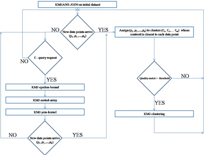
To solve this problem, we propose an algorithm called RE-JOIN. In this al-gorithm, first we perform KMEANS-JOIN on the initial data set and obtain the cluster centroids C[c1...ck] and join result according to the ε parameter. When
a number (n) of new data points p1, p2, ..., pn has started to arrive, they are
im-mediately assigned to clusters whose centroids C[c1...ck] are the closest to each
data point. Then a defined cluster quality metric (qm) is calculated and com-pared with a predefined threshold value (t). If qm exceeds the threshold t, then it means that a reclustering is required. In this case, we employ the GPU based KMJ-clustering (see Section 4.3.1) and obtain new clusters including new data points that arrived in the previous iteration. In the other case when qm is still less than the threshold t, then it means that there is no need for a reclustering. When an epsilon query with same ε parameter is requested, KMEANS-JOIN al-gorithm without KMJ-clustering is again employed to produce join results. Since we have the ε-join results of previous dataset before the updates and ε query request, a variation of KMJ-join-kernel is implemented to avoid redundant pair comparisons. Figure 4.7 gives the algorithm schema of RE-JOIN.
As mentioned earlier, RE-JOIN decides the necessity of reclustering by com-paring a cluster quality metric with a predefined threshold value. We defined total-cluster-distance-change as a cluster quality metric. It is computed as, first calculating the updated cluster centroids Cu[(cu)
1...(cu)k] after new data points
has been assigned. Then the distance between updated cluster’s centroid (cu) i
and its corresponding previous centroid ci is calculated where i = (1, 2, ..., k).
has an initial value of zero.
Chapter 5
Evaluation
In this chapter, first we give implementation specific details, dataset information and explain CUDA based challenges that we face with and optimizations that we come up with. Then, we report the experimental evaluations of proposed algorithms and make comparisons in terms of dataset size, join selectivity and running time, and discuss the results.
5.1
Implementation Details
In this Section, we give the details of datasets we use and some challenges and optimizations in CUDA programming are explained. We conduct our experiments on a NVIDIA Geforce GTx 560 GPU which includes 384 CUDA cores and has 1 GB Memory and Intelr CoreT M i5-2500 3.30 GHz processor which includes 4 Cores, 6M Cache.
5.1.1
Challenges and Optimizations
There are some performance tunings on GPUs such as global memory accesses and shared memory bank conflicts. In CUDA, there 32 banks which provide the
communication between shared memory and threads and each is responsible from a single thread and 32 bit data. If these 32 banks are assigned to different data addresses, then they run concurrently. If two different threads want to access the same 32 bits at the same time, then the bank conflict occurs. In this situation, bank provide the data to one of the threads first, and then to the other. This is a 2-way bank conflict. In CUDA, 32 threads form a warp and all the threads within a warp run in parallel. If all threads in a warp want to access the same memory address at the same time, then broadcast occurs rather than 32-way bank conflict. This provides the transferring of all required data to all demanding threads at one data transfer time. As explained in Section 4.2, in our proposed GPU-INLJ algorithm, the data is divided into a number of threads per block sized chunks and these chunks are only the half size of reserved shared memory per block. Each thread in a chunk is responsible from a 8 dimensional float type of data point (query point) and each of them wants to access every dimensions of all data points which reside in the other half of the reserved shared memory. Also each chunk contains 32 data points whose one dimension consists of 32-bits. Thus each thread access the ith dimension at the same time and broadcast occurs and 32 broadcast operations are performed rather than 32 × 32 data transfer.
The minimum number of threads per block in CUDA is same as the warp size which is 32. In general, small block size limits the total number of threads and 128 or 256 number of threads per block is sufficient. However, in our experiments, we choose the threads per block number (NTHREADS) as 32. The reason of this choice is minimizing the granularity because of the padding operation. We pad the dataset to an odd factor of NTHREADS because the main loop of GPU-INLJ algorithm operates for odd number of blocks and (number of blocks + 1)/2 steps are performed to guarantee that all pairs are compared. Thus at most (NTHREADS × 2)−1 number of padded data is required. In order to minimize this value, we choose 32 threads per block. Padded data avoids the unnecessary and expensive branch operations which are required for index and memory controls.
5.1.2
Dataset
For our experiments, we generated 8 dimensional synthetic data with varying number of data points type of float and data values ranging from 0 to 10. Since we do not use any index structure in our GPU based NLJ and INLJ algorithms, the distribution of the dataset is not important. However, for KMEANS-JOIN algorithm, since we first cluster the data, we generate clustered synthetic data which consists of ten clusters with varying number of data points. To illustrate the dataset (see Figure 5.1), first we use principle component analysis to reduce the number of dimension to 2. A dataset with 100K data points is shown in Figure 5.1.
Figure 5.1: Representation of a dataset with 100K data points
We also generate 8 dimensional synthetic data with uniform distribution and data values ranging from 0 to 10 type of float, in order to evaluate the perfor-mance of KMEANS-JOIN algorithm comparing to the GPU-based NLJ and INLJ algorithms.
Finally, we perform our algorithms on areal data set from UCI-KDD repository which is Corel Image Features Data Set We use the color moments data which
consists of 68040 data points with 9 dimensional.
5.2
Experimental Results
In our experimental results, we evaluate the performance of the proposed algo-rithms in terms of size of the dataset, ε parameter (join) selectivity, number of clusters (k) selectivity and speedup. Also we measure the number of replicated data points according to the k and ε. Experimental results are conducted on the following algorithms which solve similarity join problem:
• CPU based Nested Loop Join (CPU-NLJ) algorithm
• GPU based Nested Loop Join (GPU-NLJ) algorithm which is also men-tioned in [36]. GPU-NLJ also contains the data transfer between CPU and GPU. NLJ-join-kernel only includes the kernel function which performs join opera-tion.
• GPU based Improved Nested Loop Join (GPU-INLJ) algorithm which is our proposed work and improve the GPU-NLJ providing a communication scheme between CUDA thread blocks and increasing the shared memory usage. GPU-INLJ also contains the data transfer between CPU and GPU. GPU-INLJ-join-kernel only includes the kernel function which performs join operation.
• GPU based Partitioning and Epsilon Bound (KMEANS-JOIN) algorithm which uses k-Means clustering algorithm to partition the data and provide epsilon boundaries between partitions to avoid missing join pairs. Also it uses the GPU-INLJ algorithm in each partition to produce join results.
We also evaluate the main components of KMEANS-JOIN algorithm which are as follows:
1. KMJ-clustering: A GPU based k-Means Clustering algorithm.
that need to be replicated and clusters to which the data points are repli-cated.
3. KMJ-sorted-array: Create an array sorted by cluster id including the overlapped data points
4. KMJ-join-kernel: A GPU Kernel function which performs the similarity join operation for each independent partition. Running time measurements for KMJ-join-kernel includes the all join operations of all partitions.
5.2.1
Dataset Size
In this section, we evaluate the running time performances of proposed algorithms by varying the dataset size from 100K to 500K. In order to show the effect of dataset size, we use the synthetic clustered dataset.
Figure 5.2 compares the running time performance (including data transfers) of CPU-NLJ, GPU-NLJ and GPU-INLJ algorithms for varying dataset size, when ε is 0.5. As shown in Figure 5.2, both GPU-NLJ and GPU-INLJ are not affected by the computation load as CPU-NLJ is. The reason of this result is that each thread in GPU makes slightly less computation than CPU. However CPU makes all the computation in a single thread and variation on the data size directly affects the performance.
From Figure 5.2, we can also show that our proposed GPU-INLJ widens the spread between CPU-NLJ when dataset size is getting larger. The reason is that the GPU-INLJ is adaptive for larger data set and needs only extra one iteration, if numberof threads × 2 data point is included into the dataset. Also the effect of the dataset size for GPU-NLJ and GPU-INLJ is dramatically less than it has for CPU, because the distance calculations and comparisons which GPU perform for a thread slightly fewer than CPU does.
Figure 5.3 makes performance comparison in terms of the running times (in-cluding data transfers) of GPU-NLJ, GPU-INLJ and KMEANS-JOIN (in(in-cluding
100K0 200K 300K 400K 500K 100 200 300 400 500 600 700 800 900 1000 Dataset size Time (seconds) GPU NLJ GPU INLJ CPU NLJ
Figure 5.2: Variation of running time of CPU-NLJ, GPU-NLJ and GPU-INLJ with increasing dataset size. ε: 0.5
its all components) algorithms for varying dataset size, when ε is 0.5 and num-ber of clusters is 20. In Figure 5.3, we can see the performance improvement of GPU-INLJ better than GPU-NLJ. Although, the GPU-NLJ also includes shared memory usage, it is slower than our improved algorithm GPU-INLJ which has 2× speedup over GPU-NLJ.
100K0 200K 300K 400K 500K 20 40 60 80 100 120 Dataset size Time (seconds) KMEANS−JOIN (k:20) GPU NLJ GPU INLJ
Figure 5.3: Variation of running time of GPU-NLJ, GPU-INLJ and KMEANS-JOIN with increasing dataset size. ε: 0.5 and k: 20
As shown in Figure 5.3, KMEANS-JOIN outperforms the GPU-INLJ. In par-ticular, the running time of KMEANS-JOIN grows slower than the running time of GPU-INLJ does. Also, it is up to 5 times faster than GPU-INLJ and scales better.
Figure 5.4 displays performance comparison in terms of running times of main components of KMEANS-JOIN algorithm for varying dataset size, when ε is 0.5 and k is 20. It can be seen that the running times of all components except KMJ-join-kernel increase almost linearly with increasing dataset size. Also, in Figure 5.5 which is an inference of Figure 5.4, we give the percentage contri-bution of main components of KMEANS-JOIN algorithm in terms of running time. We can see that the percentage contribution of execution time of KMJ-clustering decreases when the dataset size getting larger, however, the percentage contribution of execution time of KMJ-join-kernel increases. All other compo-nents’ percentage contribution remain almost same. These results show that the fast convergence property of k-Means clustering algorithm and its GPU based implementation have significant impacts on the scalability of KMEANS-JOIN algorithm. Almost quadratic increase in KMJ-join-kernel is inherited from GPU-INLJ algorithm which is employed in KMJ-join-kernel. However, we will see the impact of partitioning the data on join operation.
100K 200K 300K 400K 500K 0 5 10 15 Dataset size Time (seconds) KMJ−join−kernel KMJ−epsilon−bound KMJ−sorted−array KMJ−clustering
Figure 5.4: Effect of dataset size on running time of main components of KMEANS-JOIN. ε: 0.5 and k: 20
Figure 5.5: Percentage contribution of main components of KMEANS-JOIN al-gorithm in terms of running time. ε: 0.5 and k: 20
We also give the speedup results of proposed algorithms for varying number of dataset size. Table 5.1 shows that KMEANS-JOIN significantly outperforms all other algorithms and is up to 4.7 times faster than GPU-INLJ algorithm. We can also see from Table 5.2 that, GPU-INLJ has up to 13 times performance improvement by CPU-NLJ. Finally we parallelize the CPU-NLJ algorithm by using OpenMP (OMP-CPU-NLJ) on a system mentioned in 5.1and show that it is up to 2 times faster than serial code.
Table 5.1: Speedup of KMEANS-JOIN algorithm over CPU-NLJ, GPU-NLJ, and GPU-INLJ for varying dataset size
100K 200K 300K 400K 500K KMEANS-JOIN over CPU-NLJ 18.65 36.70 42.30 54.40 65.15 KMEANS-JOIN over GPU-NLJ 3.02 4.61 4.96 6.21 7.37 KMEANS-JOIN over GPU-INLJ 1.82 3.07 3.22 3.98 4.69