Change detection in digital video signals

A T H E S I S

S U B M I T T E D T O T H E D E P A R T M E N T O P E L E C T R I C A L

A N D

E L E C T R O N I C E N G I N E E R I N G

A N D T H E I N S T I T U T E O F E N G I N E E R I N G A N D S C I E N C E S

O F B I L K E N T U N I V E R S I T Y

I N P A R T I A L F U L F I L L M E N T O F T H E R E Q U 8 R E M ¿ N T S

5^ ^

F O R T H E O E G R E : E E ' O f ·

N '' · '

M A S T E R O F S C I E N C E

R a b i Z a i b i

D e c e m b e r 1 9 9 9

■135

/393

CHANGE DETECTION IN DIGITAL VIDEO

SIGNALS

By

Rabi Zaibi

December 1999

τ <

é é < ¿ o . < r

I certify that I have read this thesis and that in my opinion it is fully adequate, in scope and in quality, as a thesis for the degree of Master of Science.

7

'

Prof. Dr. A. Enis Çetin(3upervisor)

I certify that I have read this thesis and that in my opinion it is fully adequate, in scope and in quality, asia thesis for the degree of Master of Science.

I certify that I have read this thesis and that in my opinion it is fully adequate, in scope and in quality, as a thesis for the degree of Master of Science.

^^ssoc. Prof. Yasemin Yardımcı Çetin

Approved for the Institute of Engineering and Sciences:

Prof. Dr. Mehmet Bar^

Director of Institute of Engineering and Sciences

ABSTRACT

CHANGE DETECTION IN DIGITAL VIDEO

SIGNALS

Rabi Zaibi

M.S. in Electrical and Electronics Engineering

Supervisor: Prof. Dr. A. Enis Çetin

December 1999

We present a method for scene change detection based on projections onto the vertical, horizontal and diagonal axes. At first, vertical projection of each two consecutive interframe differences are calculated. Then based on the dis­ tance measure between them, together with proportionality and sign tests, fade in/out, dissolve, wipe and cut can be classified. We also propose a method for small moving object detection in video sequences based on adaptive prediction and higher order statistical tests. We first eliminate camera movement using subpixel accurate motion estimation. Then adaptive prediction is applied on the image obtained from motion compensation and an error image is obtained. Higher order statistical test is then applied on the residual image to detect small moving objects whose size may consist of only a few pixels.

Keywords: Shot Transition, Projection, Moving Object Detection, HOS, Adap­ tive Filtering

ÖZET

SAYISAL VİDEO SİNİYALLARINDAKİ DEĞİŞİMİN TESPİTİ

Rabi Zaibi

Elektrik ve Elektronik Mühendisliği Bölümü Yüksek Lisans

Tez Yöneticisi; Prof. Dr. A. Enis Çetin

Aralık 1999

Modern bilgi sistemlerinde sayısal video analiz teknikleri önemli bir rol oyna­ maktadır. Video analizdeki önemli aşamalardan biri, sönüşüm ve erime gibi video geçişlerinin tespit edilmesidir. Çeşitli video geçişlerin tespiti için, yatay, düşey ve yatık eksenler üzerindeki izdüşümlere dayalı yeni bir metod sunmak­ tayız. Küçük hareketli hedeflerin tespiti için de yeni bir metod önermekteyiz. Başta, devinim dengelenme algoritması kullanarak, kameranın hareketini ele­ mekteyiz. Sonra, küçük hareketli hedeflerin tespiti için devinim dengelenmesin­ den edinmiş resimlere, uyarlamalı süzgeçlerne, altband ayrıştırma, ve yüksek dereceli istatistiklere dayalı testler uygulamaktayız.

Anahtar Kelimeler. Video sahne geçişin tespiti, İzdüşümler, Hareketli hedef­ lerin tespiti. Uyarlamalı süzgeçlerne, Altband ayrıştırma. Yüksek dereceli is­ tatistikler.

ACKNOWLEDGMENTS

I would like to use this opportunity to express my deep gratitude to my su­ pervisor Prof. Dr. A. Enis Çetin for his guidance, suggestions and invaluable encouragement throughout the development of this thesis.

I would also like to thank Prof. Dr. Levent Onural and Assoc. Prof. Dr. Yasemin Yardımcı Çetin for reading and commenting on the thesis.

Finally, many thanks to all of my close friends Nabil .Jmel, Khaled Ben Fatma, Gena Lopez, Elmarine Williams, Yavuz Selim Kömür, Gökhan Süt, Batur Orkun and other non-listed friends for their moral support.

Contents

1 INTRODUCTION 1

1.2 Scene Change detection... 2

1.3 Detection of Small Moving Object 5 1.4 Thesis O utline... 7

2 PROJECTIONS BASED SCENE CHANGE DETECTION 9 2.1 Different types of shot tra n s itio n s... 10

2.2 Projection of two-dimensional discrete signals 12 2.3 Scene Change Detection using P ro je c tio n s ... 15

2.3.1 Production Characteristics of Video Sequences... 15

2.3.2 Detection Algorithm for Dissolve and F a d e ... 17

2.3.3 Detection Algorithm for Cut and W ip e ... 19

2.3.4 Experimental R esu lts... 21

3 SMALL MOVING OBJECT DETECTION IN VIDEO SE­

QUENCES 23

3.1 Motion A nalysis... 25

3.2 2-D Adaptive P re d ic tio n ... 26

3.2.1 Review of 1-D filte rin g ... 26

3.2.2 2-D Adaptive F ilte rin g ... 27

3.3 Higher Order Statistical T e s t... 30

3.4 Linear Subband Decomposition 33 3.5 Adaptive Subband Decomposition 35 3.6 Experimental R e su lts... 36

4 CONCLUSION 41

A MATLAB code for the detection of small moving objects 52

List of Figures

2.1 Various shot transitions: (a) cut, (b) fade in, (c) fade out, (d)

dissolve, (e) wipe. 11

2.2 Illustration of projection onto the horizontal axis... 13

2.3 Illustration of projection onto the vertical axis... 14

2.4 Illustration of projection onto the oblique axis... 14

2.5 Distance between qi's. 17

2.6 The overall classification diagram. The distance measure D is

defined in Equation 2.8. 18

2.7 Projection of the interframe difference images: (a) first projec­ tion vector Qi, for the first two frames, (b) projection vector ^¿+i

for the next two frames. 20

3.1 Overall detection scheme using adaptive prediction.

3.2 Adaptive filtering structure

24

27

3.3 2-D adaptive filter s tr u c tu r e ... 28

3.4 Region of support (ROS) of the adaptive filter... 29

3.5 (a) a frame containing a small moving object (b) the following frame (c) the error image after 2-D adaptive filtering 29

3.6 Scanning direction in adaptive filtering... 30

3.7 Illustration of overlapping windows... 31

3.8 Comparison between the detection performance of each method: (a) original image containing a small moving object, (b) the residual error image, (c) detected regions using the CA-CFAR technique, (d) detected regions using simple thresholding, (e) detected region using the HOS test... 33

3.9 Subband decomposition structure... 34

3.10 Linear subband decomposition: (a) original image, (b) (c) xih... 34

3.11 Adaptive subband decomposition structure. 35

3.12 Adaptive subband decomposition: (a) original image x, (b) x;/i, (c) Xhi... 37

3.13 (a) A frame containing a moving small object, (b) the following frame, (c) the result of motion compensation, (cl) prediction eiror image e[?n,77.] and the detected region (right), (e) sum of the subimages Xih[m,n] and Xhi[m,n\ and the detected region (right), (f) sum of the subimages xu\m , n] and n] obtained after adaptive subband decomposition and the detected region (right)... ₃₉

List of Tables

2.1 Detection performance of the projections based shot transition detection method... 21

3.1 Detection performance of each method... 32

3.2 Values of the test statistic h ( / i ,/2,/3,/4) in regions with and

without moving objects. 33

3.3 Detection performance of each method... 39

Chapter 1

INTRODUCTION

During the last decade due to the advances in computer technology, informa­ tion technology has made hyperfast progresses making digital information very common in various aspects of life. As a matter of fact, digital video has spread to nearly all the fields of modern information systems like communication, education and surveillance.

Video is a medium with high resolution and very rich information content. Besides the meta-data like the author, the production date, the title, video provides other information based on its content, like sounds, events, places and the like. We can define a video clip as a sequence of pictures (frames) that are displayed at a pre-specified rate [1].

Digital video data is different from textual data in that it has both spa­ tial and temporal dimensions. Moreover, it is difficult to analyze, to manage, to access and to reuse video sequences due to the high volume and to their unstructured format. Consequently, video analysis need to be performed on

smaller sequences known as shots. A video shot is the basic unit for video understanding. It is a single sequence of a motion picture or a television pro­ gram shot by one camera without interruption, i.e., it consists of a sequence of frames which represent a continuous action in time and space [5].

Several methods have been developed for digital video data analysis [9,10, 13]. Their application vary from video coding [15,16,48] to video parsing [4] and indexing [26-28] for use in emerging multimedia applications [15] and video databases [31]. Most of these methods are based on extracting important features of video such as object motion, scene change, color or sound [2,8,15, 19,34].

Given that frames within video sequences generally vary with time, detect­ ing the change in these frames with respect to time provides a good method for video analysis. The change within the frames can be due to scene changes done by the shooting camera or due to the movement of the objects within them. In this thesis, we propose two methods for change detection in video sequences, the first aimed at detecting scene changes and the second for detection of small moving objects.

1.2

Scene Change d etection

Scene Change Detection (SCD) is also known as shot transition detection. Within a video sequence, the consecutive frames may differ from each other due to object or camera movement, lighting changes, gradual changes (continuous cuts) or abrupt changes (camera cuts, discontinuous cuts) [6]. Gradual changes include several effects like wipe, fade in/out and dissolve.

Scene Change Detection is usually based on some measurements of the image frame, which can be computed from the information contained in the frames. This information can be color, spatial correlation, object shape, motion contained in the video image, or DC coefficients in the case of compressed video data [1]. In general, gradual scene changes are more difficult to detect than abrupt scene changes and may cause major scene chnage detection algorithms to fail under certain circumstances [11].

Existing scene change detection algorithms can be classified in many ways according to the video features they use and the video objects they can be applied on, among other factors. Most of them rely on using the dissimilarities between consecutive frames.

One of the methods used for scene cut detection is based on comparing the interframe difference to a given threshold, after applying camera motion compensation on the frames [17]. Some of the difference measurement functions can be color histogram and gray level histograms [6].

A gradual SCD algorithm is more challenging than its abrupt counterpart, especially when there is a lot of motion involved. Unlike abrupt scene changes, we cannot use the sharp peaks in the inter-frame difference sequence to detect them and are easily confused with object or camera motion. Gradual scene changes are usually determined by observing the behavior of the inter-frame differences over a certain period of time.

Some approaches use a combination of speech and visual data for video shot classification [2,12,34]. In [34], the use of the projection of two-dimensional signals for video scene change detection was introduced. Some other approaches

provide fast methods for scene change detection in the compressed environment [10].

In [-3], W.Wolf and H.Yu use edge detection and calculation of the centroid and the variance of the differencing regions for detection of wipe transition. In [6], Yu, Bozdagi and Harrington proposed a feature-based algorithm for fade and dissolve detection which takes advantage of the production aspects of video. It represents the intensities in the frames as a function of time, based on which fade and dissolve can be distinguished from zooms and pans. Another method uses wavelet analysis of the frames for detection of gradual scene changes like fade and dissolve [5].

For compressed video data, [14] presents a scene change detection algorithm based on the generalized sequence trace. Features are first extracted from the DCT coefficients, from which a generalized sequence trace is obtained. Then it uses thresholding technique on the dissimilarity measures between the elements of the trace for deciding on the existence of scene changes.

The method we present relies on projections on horizontal, vertical and oblique axes for various scene change detection. It enables the detection of five types of transitions namely, fade in/out, dissolve, wipe and cut at once and with a very low computational complexity. This idea is originally mentioned in [34]. Independently, in [7], Min Wu et al. presented a method which uses the vertical projection of the interframe difference image for the detection of horizontal wipes. It is based on the assumption that between the wiping scenes a border of pixel value 255 shall exist from which wipe transition regions have the property that their standard deviation is the highest compared to other transitions.

1.3

D etection of Small M oving O bject

A second topic that is studied in this thesis is the detection of small moving objects which can be a complicated task when there is noise and the video camera is in motion. This is not only important in video data querying and retrieval but also has a wide range of applications from surveillance systems to target detection schemes in defense systems. Most of the object segmentation methods [15,17,18, 20] are geared for large objects with clear features and boundaries whereas in our problem the moving region or object may consist of only a few pixels.

In [15,17], a method which uses a fusion of both single frame based col­ or segmentation using an improved recursive-shortest-spanning-tree (RSST) method [18] and motion segmentation from consecutive frames for the detec­ tion and the tracking of objects of rather large sizes was presented. It proved efficiency for emerging multimedia applications like in video conferencing.

Several methods for detection of moving objects ^ ^ for use in surveillance and defense systems were developed [21-26,60]. In [21], R. T. Collins et al presents a video surveillance and monitoring system (VSAM). It uses a dynamic background subtraction method to extract and track objects. In this method, the background is assumed to have Gaussian distribution and is adapted ac­ cording to small changes. An object is detected if the change in the background exceeds a certain threshold. This method is prone to erroneous extraction of the moving object and to high changes in background not due to a moving

‘http://www.sloan.salk.edu/~wiskott/Bibliographies/MotionAnalysis.html '■‘http://www.sic.rina.ac.be/~dirk/DEMOS/detect/moving.targets.html

object, i.e., trees blowing in the wind. It is applicable only for the case of fixed camera.

Another fixed camera based object detection algorithm for use in surveil­ lance systems is presented in [26]. This method detects the change in the con­ secutive frames using interframe absolute differencing. This method produces false alarms in cases where a non moving object is added to the background without aiming to detect it and is also used for detection of objects of rather large sizes.

Some approaches for target detection based on optical analysis ^ are pre­ sented in [55-57,59]. In [54], Aggarwal et al presents a method for Automatic Target Recognition (ATR) in Forward Looking Infrared (FLIR) images. The approach is based on modeling the background using Gaussian and Weibul- 1 functions from which targets, usually, military vehicles are distinguished. These targets are then recognized from a preset list of objects.

Another method for the detection of targets in still images taken by a natural light camera is described in [55]. The elements of the background such as vegetation are first clustered using statistical clustering techniques like the Linde-Buzo-Gray (LBG) clustering method, from which any anomalies can be detected using the background suppression filtering. This algorithm can achieve good results but is prone to abrupt changes in the background and is environment dependent , i.e., it fails in a desert environment.

Several methods enable the tracking of multi-targets in very cluttered FLIR images [58]. A sequence of images obtained from an IR sensor are first stacked

^http://www.aic.nrl.navy.mil/~kamgar/frame.html '‘http://robotics.stanford.edu/~bwang/ATR.html

in a unique image. The single frames contain binary pixels, i.e., pixels belonging to a clutter or a moving object are set to 1 otherwise they are zero. The pixels in the track of the object are usually correlated. Based on that assumption, a modified high order correlation function is calculated for pixels neighboring each other and a hard limiter threshold function is used to decide on the pixels to be belonging to a track or a clutter.

In [56], R. S. Caprari introduces a moment based method for the detection of targets in images. This is based on the assumption that the shape of objects is different from the shape of the elements of clutter in the output image of the correlation filter and a moment analysis would distinguish them.

We present a method for small moving object detection, which relies on adaptive filtering, subband decomposition and higher order statistical (HOS) tests. It is applicable for cases where the camera is fixed or moving and it is computationally efficient.

1.4

Thesis Outline

In Chapter 2 we propose a new method based on projections onto horizon­ tal, vertical and oblique axes to detect scene changes, such as fade in/out, dissolve and cut. This method has the computational advantage of reducing two-dimensional signals (frames) into one dimensional vectors for the detection of transitions.

Our method mainly uses the projections of the interframe difference sig­ nals. For instance, in case of cut and wipe transitions, the distance between

the projection vectors for two consecutive interframe difference images is much different than in case of dissolve and fade. Then using the production charac­ teristics of the video data we can identify the different types of transitions.

In Chapter 3 we propose a new method for detection of small moving ob­ jects in video sequences. We first describe subpixel motion we use the LMS prediction error image together with higher order statistical (HOS) tests, to detect a moving object of relatively small size. We also use adaptive and simple subband decomposition techniques in conjunction with HOS tests to achieve the same task. Finally, we compare the different methods according to their precision in detecting small moving objects by carrying out some experimental studies and also according to their computational complexity.

Chapter 2

PROJECTIONS BASED

SCENE CHANGE

DETECTION

In this chapter we discuss the basic elements of shot transition. Then we dis­ cuss the new scene change detection (SCO) algorithm based on projections onto horizontal, vertical, and oblique axes of two-dimensional signals (frames). The approach of using projections to detect scene changes was first introduced in [34]. However, not much details were given about how that can be achieved. Our thesis work started in 1997 on the development of that approach. Inde­ pendently, in [7] M. Wu, W. Wolf and Bede Liu introduced a method for wipe detection using statistical information from the projection of the inter-frame differences, in 1998.

Generally speaking, there are two types of shot transitions, abrupt (dis­ continuous) including cut transition and gradual (continuous) shot transition including fade, dissolve and wipe transitions [5,7].

A shot is a single sequence of motion picture or a television program shot by one camera without interruption. In other words, it consists of a sequence of frames which represent a continuous action in time and space. It is the basic unit for video understanding. A list of key-frames extracted from the shots of a video clip can give the user a rough idea about the story of the video clip and are usually used for video content analysis. Technically, shot transition detection can be done by the analysis of a time-varying characteristic function of the frames [3]. Figure 2.1 gives a brief idea about the four different shot transitions to be discussed in this chapter: abrupt scene change (cut) and gradual scene changes (fade in/out, dissolve and wipe).

2.1

Different types o f shot transitions

A fade of a video sequence is a shot transition with the first shot gradually disappearing (fade out) before the second shot gradually appears (fade in); and a dissolve in a video sequence is a shot transition with the first shot gradually disappearing while the second shot gradually appears [5] (see Figure 2.1). On the other hand, a wipe transition is a transition from one scene or picture to another made by a line (a curve or polygon) moving across the screen. Visually, we can see one scene is gradually moving out of the picture while another scene gradually disappears. From the production point of view, one part of the original image is replaced by another fragment from another

(a)

(c)

Figure 2.1: Various shot transitions: (a) cut, (b) fade in, (c) fade out, (d) dissolve, (e) wipe.

image. In other words, during a wipe, one portion of the frame has a much more significant difference than the rest portions of the frame when it is compared to the previous frame on a pixel by pixel level differencing. It is a result of the continuity of the shot.

2.2

P rojection of tw o-dim ensional discrete sig­

nals

We can define the projection of discrete signals as an arrangement of the sam­ ples from an R-dimensional sequence into a Q-dimensional sequence [.32]. In [18] and [1], a description of the projections of 3-D real world scenes onto 2-D im­ ages is given. In our work, we focus on the projection of 2-D images onto the horizontal, the vertical and the oblique axes.

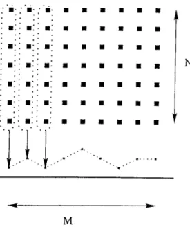
• Projection onto the horizontal axis; given an image /j taken from a video sequence and of size M x N, the projection of fi onto the horizontal axis, also known as vertical projection is defined as

E fi{m ,n) \< m < M (2.1)

Figure 2.2 illustrates the projection on the horizontal axis, in which the elements of the column are summed up to give the projection at point m.

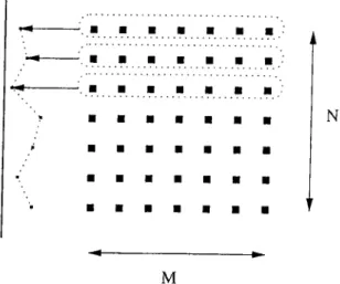
Projection onto the vertical axis is the projection 'Ph,i of frame /j onto the vertical axis, also known as horizontal projection and is defined as

l< n < N (2.2)

N

M

Figure 2.2: Illustration of projection onto the horizontal axis.

Figure 2.3 illustrates the horizontal projection, in which the elements of the row are summed up to give the projection at point n on the vertical axis.

• Projection onto the oblique axis: the projection po,i onto the oblique axis is the projection of frame /j onto an axis at angle 6 = 45°:

(2.3)

as shown in Figure 2.4.

N

M

Figure 2.3: Illustration of projection onto the vertical axis.

M

N

Figure 2.4: Illustration of projection onto the oblique axis.

2.3

Scene Change D etection using Projections

In this section we describe the way horizontal, vertical and oblique projections, Ph, Pv and po respectively, are used to detect shot transitions. This is mainly based on using the production characteristics of video to compare consecutive frames.

Generally, wipes are the most difficult transition types to detect because there is a wide range of wipe types like simple wipes with vertical border, star wipes and polygonal border wipes [3]. Fade transition detection is also a difficult problems as in some cases images fade to black whereas in other cases they fade to white. So it is important to make some assumptions on the production characteristics of these gradual video shot transitions.

2.3.1 P rod u ction C haracteristics o f V ideo Sequences

As there exists a wide range of gradual shot transitions, it is necessary to make some assumptions on the general production characteristics of the video sequences, with which our proposed algorithm works properly. For fade, we suppose that the transition occurs at a constant rate, that is the difference between the pixel levels of two consecutive frames /j and /¿_i shall be constant;

*^i+l /t+1 ft — — ft fi — l (2,4)

For fade in, the frame have pixel values higher than the (i — frame, and for fade out it is the opposite. As we suppose that the very first image in a video sequence containing fade in is a black image with pixel values equal to

zero. Each image frame shall be proportional to the difference image as follows

fi = a x di a > 1 (2.5)

In dissolve, we suppose that the transition occurs at the same rate. In which a fading in image superposes a fading out image, both at the same rate. For wipe we suppose that it is occurring at a constant rate and that the border between the two images forming the frames is linear as shown in Figure 2.1 (e).

The border slides to show more of the first image and taking place on the second image which gets reduced from frame to the next frame at a constant rate. The projections qi of the difference images play a major role for the projections shot transition detection algorithm. These projections of difference images with size M x N are defined as follows

N

QvA '^ ) = (2.6)

for vertical projection and

n=l

M

Q.h,i. i { " ) = 5 3 (2,7)

m=l

for horizontal projection. Qi's shall all be constant throughout a fade and dissolve transitions whereas they can take variable values throughout a wipe or cut transitions. More specifically, the distance between Qi and gj+i shall be almost zero for fade and dissolve, and different from zero for wipe and cut. Figure 2.5 shows the distance between gj’s for a video sequence containing in the following order: dissolve, fade in, wipe, cut and fade out.

Distance between the intertrame difference vectors

Figure 2.5: Distance between Qi's.

2.3.2

D etection A lgorithm for D issolve and Fade

Given three consecutive frames, /¿_i, ft and /¿+1, we calculate the interframe differences di = fi — fi- i and dj+i = fi+i — fi- We then calculate the projections of these interframe difference matrices onto the horizontal axis to obtain qy^i and Qv^i+i, onto the vertical axis, to obtain the vectors Qh^i and qh,i+i, respectively, and on the oblique axis to obtain and qo,i+i- We use these vectors to distinguish between fade and dissolve on one side and wipe and cut on the other side. This can be achieved by calculating the distance between qi’s. If the distance takes values below a threshold T^i throughout a transition then the transition can be classified into the fade and dissolve category, otherwise it can be classified in the wipe and cut category. The distance between qi and qi-i, is defined as:

D{qi ,qi -i ) = \ \ qi - qi - i \ \ (2.8)

1-1

1+1

Figure 2.6; The overall classification diagram. The distance measure D is defined in Equation 2.8.

The next step is represented in separating dissolve from fade in and fade out. As we have already explained, in case of fade in, the frame fi has pixel values higher than the {i - 1)‘* frame /j_i, consequently, all the elements of the difference matrix di must be positive. In a similar way, for the case of fade out the difference matrix di has negative elements.

The separation of fade in, fade out, and dissolve according to the sign of the interframe difference matrix might not be sufficient as in dissolve we can have either totally negative or totally positive elements for the difference matrix, or both of them , depending on the pixel values of the fading in image superpos­ ing the fading out image. This can be done by checking the proportionality constant defined in Equation 2.9.

According to proportionality assumption made on the production charac­ teristics of fade and dissolve, we need to check whether the three selected frames conform to this assumption or not. This can be achieved by checking whether the projection vector of frame fi is proportional to the projection vector qy^i of the difference matrix:

Q.v,i — ^^'P v,i (2.9)

where a > 1.

If Equation 2.9 is satisfied and that and have completely positive elements then the transition from the {i - frame to the {i 4- frame is a fade in, else if Qh^i and q/i^i have completely negative elements then the transition from the {i - ly ^ frame to the {i + 1)^'* frame is a fade out. If the above two cases do not take place then the transition can be considered a dissolve. However the above assumption might not apply in some cases where the interframe difference is very low and so some transitions which are neither fade nor dissolve are classified in the fade/dissolve category.

2.3.3

D etection A lgorithm for Cut and W ipe

Cut transition is the easiest to detect. As we have previously explained cut and wipe fall in the same category in the way that for three consecutive frames, cind fi+i, Qi’s are generally very different from each other as shown in Figure 2.5. Any other type of non-horizontal wipes [4,5] are not detected by our .algorithm.

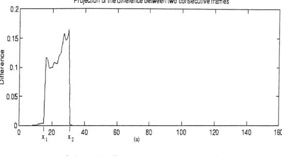
If after the fade and dissolve test, no fade or dissolve were detected then if by the wipe test no wipe is detected the sequence can be considered to contain a cut. The detection of wipe is based on the assumption we made on the production characteristics of video containing wipe. In wipe, a scene is entering and another scene is leaving at a constant rate. Figure 2.7 shows vectors Qi and Çj+i for three consecutive frames, /¿_i, fi and fi+i.

Projection of the difference between two consecutive fram es

Projedion of the difference between next two consecutive frames

Figure 2.7: Projection of the interframe difference images: (a) first projection vector Qi, for the first two frames, (b) projection vector qi+i for the next two frames.

Transitions Fade in Fade out Dissolve Wipe Cut Wrong detections 0 2

Table 2.1: Detection performance of the projections based shot transition de­ tection method.

As we can see from this figure, the elements of the projection vector Qi ideally take zero value until point Xi then take high values from Xi to X2

and finally zero values until the end of the frame. For the determination of points Xi, X2, Xz and x,\ a threshold T/j2 might be needed. Points considered to

have high values shall exceed this threshold. The same characteristics can be observed for and points xz and x^. \i x^ — x\ = xa — xz and that 0:3 = X2

then we can decide that it is a wipe transition. If these conditions are not satisfied then we can decide on the transition to be a cut.

2.3.4

E xperim ental R esults

In this section we present the simulation studies. At first, thresholds T^i and T/i2 described in Sections 2.3.2 and 2.3.3 are obtained from a training set of 20 video sequences. The calculated values for these thresholds are: Thi = 40 and Th2 = 0.03.

In the second step, we tested our algorithms on 80 video sequences con­ taining fade, dissolve, wipe and cut transitions. The interframe differences are first obtained. Then, projections on horizontal, vertical and oblique axes are

performed on them. Using these projection vectors, the clas.sification process shovi^n in Figure 2.6 is applied to separate fade and dissolve on one side and wipe and cut on the other side.

In the third step, fade and dissolve are separated according to the pro­ portionality and sign tests described in Section 2.3.2. In a similar way, the algorithm described in Section 2.3.3 is applied on the frames classified in the wipe and cut category.

Typical results of the above algorithms are presented in Table 2.3.4. As we can see from Table 2.3.4 we had no wrong detection of fade in, fade out and dissolve and had two wrong detections for wipe and cut. The wrong detection of cut was obtained in two cases where a cut with very low interframe difference was categorized in the fade/dissolve category. Two wipe transitions were wrongly detected as cuts. This is in a case where the sliding scenes are changing drastically during wipe.

The wipe detection method presented in [7] works only for cases in which there is a white border between the wiping scenes. Consequently, wipe tran­ sition has the highest- statistical values compared to other transition types. Based on this assumption, wipe detection is possible. However, we don’t al­ ways have this white border in the wipe transitions used commonly in video sequences. Our method has the advantage of overcoming this restriction in addition to the capability of distinguishing several types of transitions at once.

Chapter 3

SMALL MOVING OBJECT

DETECTION IN VIDEO

SEQUENCES

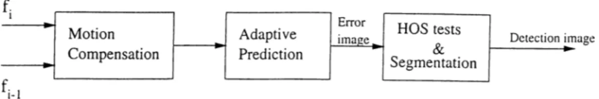
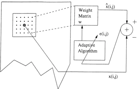
In this chapter, we present a method for detection of small moving objects in video sequences. In our approach, we first eliminate camera motion by using motion compensation [1,17,47,49-51,53]. We then use an adaptive predictor to estimate the current pixel using neighboring pixels in the motion compensated image and, in this way, obtain a residual error image. Small moving objects appear as outliers in the residual image and are detected using a statistical Gaussianity detection test based on higher order statistics. It turns out that, in general, the distribution of the residual error image pixels is almost Gaussian. On the other hand, the distribution of the pixels in the residual image deviates from Gaussianity in the existence of outliers. The block diagram of our method is shown in Figure 3.1. Instead of adaptive prediction, we also considered

Figure 3.1: Overall detection scheme using adaptive prediction.

the use of wavelet transform [46] and adaptive subband decomposition on the image obtained from motion compensation and use the same statistical test for detection of moving objects in the subimages.

The use of adaptive filtering based higher order statistical tests might pro­ vide a good method for the detection of moving objects of small sizes. The method we propose uses two-dimensional (2-D) adaptive filtering and a Gaus- sianity test [36,37] developed by Ojeda, Cardoso and Moulines (OCM) [36,41]. In this method, the image is analyzed block by block. After applying adaptive prediction, a statistic of the prediction errors is estimated in the current block to determine whether the block contains a moving object or not.

The distribution of the pixels of the residual prediction error image is ex­ pected to be Gaussian in regions where there are no moving objects and to deviate from Gaussianity in regions where a moving object exists. In Section 3.2.1 we will explain the adaptive filtering concept. Then we will extend the 1- D adaptive filtering method to 2-D dimensional signals in Section 3.2.2. Finally we will introduce the OCM tests in Section 3.3.

3.1

M otion A nalysis

Some of the video sequences we study are shot using a moving camera. In this case motion compensation is necessary, mainly to help remove redundant clutter in the background and to emphasize the moving regions in the image sequence. Many motion compensation methods have been developed in the literature. Most of them rely on the simple block and the overlapping block matching technique [1,15,17,18,50,52]. This method is very common for motion estimation due to its simplicity and effectiveness though its computational cost is high.

One of the methods that give good motion estimation is the subpixel accu­ rate motion estimation technique [17]. The input frames are first upsampled then linearly interpolated using the interpolation filter with coefficients:

hint —

The block matching technique is then applied to find an estimation of the motion of background. We use the estimated motion of the background to compensate for the camera motion. Three blocks inside the image are chosen at random, and the motion of these blocks is estimated. Best fitting displacement vector is the one that causes the least Mean Absolute Error (MAE or MAD) [51]. The MAD for a block A of size M x M inside the current frame, compared to a block В of distance {a, P) from A in the previous frame is given as:

1 ^ M A D (a ,p ) = \fi[ m ,n ] - fi- i[ m + a ,n +P]\ (3.1) 0.25 0.5 0.25 0.5 1.0 0.5 0.25 0.5 0.25 m , n = l 25

The motion vector, [a*,^*] is found by minimizing MAD(q:,/?). The motion

compensated image x[rn,v] = /¿[m,n] - /¿_i[rn + a \ n + p*] is then used in the detection procedure.

3.2

2-D A daptive Prediction

The main difficulty in detecting targets moving on various backgrounds is the suppression of background clutter which may depict different characteristics within the same sequence and even within the same frame. The use of an adaptive filter which updates itself to changing conditions [35] in the image would be beneficial in cases where the background clutter is significant and space varying.

3.2.1

R eview o f 1-D filtering

Adaptive filtering is commonly used in many areas of signal processing and communications since 1960’s [36]. The coefficients of the adaptive filter are updated according to the nature of the input signal [42]. It achieves this by adjusting its coefficients according to the feedback obtained by comparing desired response and the filter output. Figure 3.2 illustrates a typical adaptive filter. The output of the linear finite impulse response (FIR) filter can be written as the convolution of the input sequence x[n] and the adaptive filter weights w[n].

N - l

y[n] = ^ vj[i\x[n — i\ (3.2)

i=0

The error signal, e[n], is the difference between the estimated output, y and the desired signal, y[n].

e[n] = y[n] - y[n\ (3.3)

The Mean Square Error (MSE) is defined as

i(n) = E [e M \ (3.4)

The MSE can be minimized to obtain the optimum filter w{n). In the least mean squares (LMS) algorithm, an iterative procedure can be used [36]:

W fc + i( n ) = W A:(n) + ne[k\xk{n), n = 0 , 1 , . . .

with [X being the adaptation constant.

(3.5)

3.2.2

2-D A daptive Filtering

A new algorithm developed by French et al. for the enhancement of mammo­ gram images so that microcalcification regions [36-38] are brighter than the normal breast tissue [43], can be used for the enhancement of the background images so that the regions containing a moving object appear brighter than

Figure 3.3; 2-D adaptive filter structure

the background. In Figure 3.3, the adaptive filtering scheme in two dimensions is shown. In the adaptive filtering process, an image pixel x[m, n] at location (m, n) is predicted as a weighted average of pixels in its region of support. The region of support, TZ, of the adaptive filter is chosen as the pixels surrounding the pixel to be predicted as shown in Figure 3.4. The predicted pixel value x[m,n] is given as ni ri2 x[m ,n]= Y w ^ ^ ^ n )[ k j] x [ m -k ,n -l] , k = —Hi I = —rz2 (0.0) m = 0 , . . . , — 1, n = 0 , . . . , A^2 — 1 (3-6)

where x is the video frame of size Ni x N2, W(^rn,n) are the weight values at

(to, n), and (2ni + 1) x (2rz2 + 1) is the size of the region of support, Tl, of the

adaptive filter.

o o o

o • o

o o o

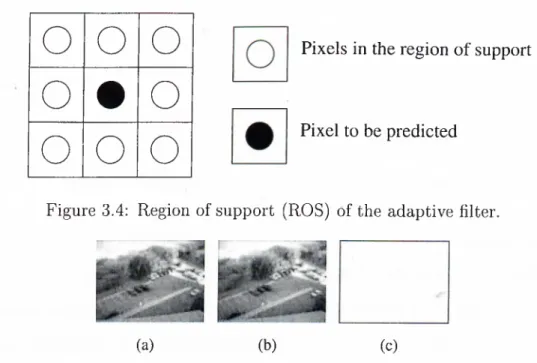
Pixels in the region o f support

Pixel to be predicted

Figure 3.4: Region of support (ROS) of the adaptive filter.

(a) (b) (c)

Figure 3.5: (a) a frame containing a small moving object (b) the following frame (c) the error image after 2-D adaptive filtering

The prediction error of the adaptive filter at location (m, n) is calculated as

e[m, n] -- x[m, n] — x[m, n] (3.7)

The weight values w^rn,n)[k,l] are adapted according to the two-dimensional LMS-type adaptation algorithm:

^ (m + l,n ) [^) ^] T ^ X e[7T i, n ] XX’[A:,/] (3.8)

where {k, 1) E TZ, and ¡j, is the adaptation constant. These weights are adapt­ ed using Equation 3.8 while processing the image in the horizontal direction. In a similar way, in the vertical direction the weight W(m,n+i)[k,l] replaces W{m+i,n)[k, 1] in Equation 3.8. In Figure 3.5 (a) and (b) a frame containing a small moving object and its following frame are shown. The image is filtered using the two-dimensional adaptive prediction filter and the resulting error image is shown in Figure 3.5 (c).

Figure 3.6: Scanning direction in adaptive filtering.

In our case, the adaptive filtering process is performed on the input image row by row as shown in Figure 3.6. The reason for the use of this zig-zag- scanning is to prevent the false jumps of the error values, that might occur at the end of the rows. In this way, smooth transition is guaranteed.

3.3

Higher Order Statistical Test

In this thesis, it is assumed that the residual signal obtained after adaptive prediction is almost Gaussian if there is no moving object. In FLIR images [54], even if the original image can be considered as Gaussian distributed in the absence of moving objects, the residual signal deviates from Gaussianity when there is a moving object. This is due to the fact that moving objects produce outliers at the object boundaries. Even if the object is small, several outliers appear after adaptive filtering as the pixels belonging to the object cannot be predicted by the neighboring pixels. Therefore, a Gaussianity detector may be used to detect small moving objects.

Higher order statistical methods are very effective in non-Gaussian envi­ ronments [37,41]. In this thesis, the OCM Gaussianity test is combined with the fourth order test developed in [36,37], for moving object detection.

Horizontal scanning

Figure 3.7: Illustration of overlapping windows.

The higher order statistic /o ,/3,/4) is based on the sample estimates of the first four moments /1, /2, /3, /4 of the prediction error [44]. Estimates of the moments are given by

.. M N

m = l n —l

where e[m, n] represents the error value at location (m, n) calculated in E­ quation 3.7 and M x N is the region in which Ik is estimated. The statistic h{Ii, /2, /3, /4) is defined as follows;

/2,/3, /4) = /3 + /4 - 3/1 (/2 - /f) - 3/| - I f +

2

In our experimental work we used blocks of size 15 by 15 where overlapping occurs at 5 pixel steps. The detection method can be considered as a hypothesis testing problem in which the null hypothesis Hq corresponds to the no moving

object case and Hi corresponds to the presence of a moving object;

Algorithm False Alarms Miss HOS 0 0 CA-CFAR 1 0 Simple thresholding 2 0

Table 3.1: Detection performance of each method.

• H,·. \ h { h j 2 j z , h ) \ < n . H,·. \ h { I u h .h J A ) \ > T ,

A classical approach is to threshold the residual signal. This will not be a robust approach because large outliers can be observed in any Gaussian process, and may cause false alarms. However, HOS based statistical test determines regions where a Gaussian behavior exists. Due to this reason, it is a robust detection method.

We compared the performance of the higher order statistical test to the performance of the Cell Averaging Constant False Alarm Rate (CA-CFAR) method [29,30], widely used in radar systems for target detection and to simple thresholding techniques on 27 image sequences and the results of this compar­ ison are shown in Table 3.1. In the CA-CFAR method, the average of each 8 pixels to the left of the pixel of interest, to its right, to its north and to its south in the shape of cross is calculated. If the intensity of the pixel of interest is higher than the calculated average then it is set to 255 else it is set to 0.

We can clearly see that the simple thresholding technique has the highest false alarm rate (2 out of 27) and the HOS test had no false alarms. The CA-CFAR method was vulnerable to significant noise. Figure 3.8 shows a comparison between the detection performance of each method.

Moving Object

(C) (d) (e)

Figure 3.8: Comparison between the detection performance of each method: (a) original image containing a small moving object, (b) the residual error image, (c) detected regions using the CA-CFAR technique, (d) detected regions using simple thresholding, (e) detected region using the HOS test.

3.4

Linear Subband D ecom p osition

Instead of adaptive prediction, the wavelet transform or subband decomposi­ tion [46] can be used. We expect that outliers corresponding to moving objects may occur in highband images and if there are no moving objects then we again expect to have Gaussian behavior.

The subband decomposition structure is shown in Figure 3.9. The input image is first processed row-wise by a lowpass and highpass filter pair and downsampled by a factor of 2. Then the resultant images are processed colum­ nwise by the same filter bank. The two most important images for our purposes are xih and Xhi which contain the horizontal and vertical edges in the original image respectively, xn and Xhh are of little interest as xu is only a smaller ver­ sion of the original image and Xhh gives no significant information about the

1-D Horizontal processing Vertical processing X Ih hi hh

Figure 3.9: Subband decomposition structure.

#

(a) (b) (c)

Figure 3.10; Linear subband decomposition: (a) original image, (b) Xhi, (c)

xih-details of the target. The two subimages xih and Xhi are useful as the lowpass behavior of the original image is no longer apparent in these images.

For example, if the background consists of a cloud, the cloud will not be visible in the subimages xih and x^i due to its low pass nature. Only the edges of the target will appear in the subimages (the edges of the cloud is expected to be removed by motion compensation). The computational cost of the subband decomposition is lower than the adaptive prediction described in Section 3.2.

U(n)

\l 2

u,(n)

Uh(n)

Figure 3.11: Adaptive subband decomposition structure.

3.5

A daptive Subband D ecom position

Another approach for processing the motion compensation image is to use adaptive subband decomposition developed in [39,40]. Adaptive subband de­ composition can be considered as a trade-off between the adaptive prediction and ordinary wavelet transform.

The adaptive subband decomposition structure [39,40] is illustrated in Fig­ ure 3.11. The structure was developed for one-dimensional signals, but we can apply it to two-dimensional signals by using the row by row and column by column filtering methods as in 2-D separable subband decomposition.

Let us first describe the 1-D procedure. The first subsignal ui is a downsam­ pled version of the original signal u, a one dimensional signal which is usually a column or a row of the input image. As ui is the result of a down-sampling by 2 operation, it contains only the even samples of the signal u. The sequence U2

is a shifted and downsampled by 2 version of u, containing only odd samples of u. We predict using Ui and subtract the estimate of-ui from U2 to obtain

the signal Uh which contains unpredictable regions such as edges of the original signal.

Various adaptation schemes can be used for the predictor P i. In our work, we used the adaptive FIR estimator, as it proved to be good for the sample images that have been tested. This adaptive FIR estimator is obtained by predicting the odd samples u^in) from the even samples Ui{n) as follows:

N N.

U2{n) = ^ to„,tti,(n - i) = ^ m„j,u(2n - 2k) _(3J1)

k = - N k = - N

where the filter coefficients Wn,k’s are updated using an LMS-type algorithm [45] as described in Section 3.2. The subsignal Uh is given by

U h { n ) = U2{ n ) - U2{ n ) (2.12)

where Uh is the error we make in predicting the odd samples from the even samples. If the motion compensated image is processed by an adaptive filter- bank we expect that small moving objects cannot be predicted as good as the other regions. Thus outliers will appear in Uh[n] in regions corresponding to moving objects.

As in the case of ordinary subband decomposition, we process the image rowwise first and obtain two subimages. Consequently, these two subimages are processed columnwise and four subimages xu, xih, Xhi, and Xhh are obtained. Figure 3.12 shows the original image x, and its subimages xih and Xfii respectively obtained after adaptive subband decomposition.

3.6

E xperim ental R esults

In this section, we present simulation studies. We test the performance of the detection scheme by analyzing 27 video sequences containing small moving

(b)

Figure 3.12: Adaptive subband decomposition: (a) original image x, (b) xih, (c)

Xhl-objects on various backgrounds. In the first step, motion compensated images are obtained. A classical block matching based motion compensation algorithm with subpixel accuracy is used [1,17].

In the second step, motion compensated images are filtered using the adap­ tive predictor and the residual error images are obtained. The values of the test statistic /i( /i,/2,/3,/4) in 12 video sequences are given in Table 3.2. It is clear from this table that a threshold can be selected which can distinguish moving objects from the background. In regions containing moving objects, the minimum value of /2,/3,/4) is 2.3 and in static regions the maximum o f h ( / i , / 2, / 3, / 4) is 0.5.

In our detection scheme we use an adaptive threshold value which is de­ termined from the first image of the video sequence according to the following formula:

,A

T/i — 0.5 ^ i ^ ^ ^2> 7^3, /4) 4" hfnax) (3.13)

where I2, h , h ) represents the value of the statistic h inside the m*'*

block, L represents the total number of blocks inside the image and hmax is the maximum value of all h ’s. In our case A is chosen as 5 so that is well above the maximum h value of the blocks containing no moving target. At first, we compare the average value havg of all h ’s inside the blocks to hmax·

Regions

With moving object Without moving object

Minimum 2.3 -0.41 Maximum 7.5 0.5

Table 3.2: Values of the test statistic h(/i, /2, /3, / 4 ) in regions with and without

moving objects.

If that average is close to hmax then we can decide on the existence of no object inside the image, else we use the value of the threshold calculated in Equation 3.13 for detection of moving objects inside the image. It has been experimentally observed that in the regions containing a target /2,/3,/4) takes its maximum value. However, we cannot take that value as a threshold because we would always come out with a detection even if no target exists, which results in false alarms. Moreover, if we just take the average value havg multiplied by coefficient T as a threshold we would always need to change A depending on the clutter remaining after motion compensation which is not very practical. The best solution for this dilemma is to take the middle value between A x havg and h.max as shown in Equation 3.13. Detection results are summarized in Table 3.3. In all of the video sequences the moving objects are determined successfully.

We also compared the performance of the adaptive predictor to the wavelet transform, and adaptive subband decomposition [39]. Motion compensated images are analyzed using (i) the adaptive predictor described in Section 3.2, (ii) wavelet transform (subband decomposition), and (iii) adaptive subband decomposition [39].

Typical results of the above methods are shown in Figure 3.13. The detec­ tion performance of these methods are summarized in Table 3.3. The adaptive

(0

Figure 3.13: (a) A frame containing a moving small object, (b) the following frame, (c) the result of motion compensation, (d) prediction error image e[m, n] and the detected region (right), (e) sum of the subimages xih[m, n] and n] and the detected region (right), (f) sum of the subimages xih[m, n] and xw[m, n] obtained after adaptive subband decomposition and the detected region (right).

Algorithms False Alarms Miss Adaptive prediction 0 0 Adaptive wavelet 2 0 Wavelet transform 0 4

Table 3.3: Detection performance of each method.

predictor produces the best results. Adaptive subband decomposition also de­ tects all of the moving objects but, in two cases, it produces false alarms. By raising the threshold we can avoid false alarms but in that case we would miss some parts of mid-sized targets. In ordinary wavelet transform, 4 targets are missed. By reducing the threshold all of the targets can be detected but in this case, the number of false alarms drastically increases.

Chapter 4

CONCLUSION

In the first part of this dissertation, we present a method based on projections on horizontal, vertical and oblique axes for detection of shot transitions like fade in/out, dissolve, wipe and cut. It is based on the use of the projection of the interframe difference to classify fade and dissolve in a category and wipe and cut in another category. In literature, several methods have been developed for detection of various types of scene changes [3-6,34]. Most of them focus on a single type of transition, i.e., wipe with its various types [4,5], dissolve [6] and cut [14].

The method we proposed has the advantage of distinguishing five types of transitions, namely fade in/out, dissolve, wipe and cut at once. Moreover, it is computationally efficient as it reduces the computational complexity by performing processing on one dimensional signals instead of two-dimensional ones. Our algorithm has been tested on 100 video sequences and only in 4 cases it detected shot transitions wrongly. Though no scene change existed, in

two cases where the interframe difference was very low, a dissolve was wrongly detected. Also, two horizontal wipes in scenes containing lots of motion were wrongly detected as cut.

Our algorithm might not also detect correctly a transition, if it is not con­ tinuous throughout three consecutive frames, i.e., if we have between two con­ secutive frames a gradual transition, and between the next two frames another type of transition, our algorithm might detect this as a cut when it is not. The method we proposed has robustness to noise in case of wipe transition.

In the second part of this thesis, we proposed a method for small moving object detection. At first we eliminate camera motion using motion compen­ sation. We used the subpixel accurate motion estimation [17] algorithm to achieve this. Then 2-D adaptive prediction, wavelet transform and adaptive subband decomposition [39] are applied on the image obtained from motion compensation. Finally, higher order statistical tests [36,37] are performed on the residual error image and subimages obtained from adaptive prediction and subband decomposition respectively to detect small moving objects.

Many moving object detection algorithms were developed in literature but they are generally geared for large size objects with clear edges and details [15- 18]. In [21,24,26], object detection algorithms for use in surveillance systems were developed. However, these methods rely on video sequence shot from a fixed camera and are especially used for large sized objects. In our problem the moving object may consist of only few pixels. In such a case, it would be adequate to find the location of these objects and not the exact edges.

Our method was tested on 27 video sequences and the adaptive predictor produced the best results. Adaptive subband decomposition also detects all of the moving objects but, in two cases, it produces false alarms. In ordinary wavelet transform, 4 targets are missed. By reducing the threshold all of the targets can be detected but in this case, the number of false alarms drastically increases. We also showed that the higher order statistical method we described earlier in this thesis performed better than the CA-CFAR method [29,30], and simple thresholding.

Bibliography

[1] A. M. Tekalp, Digital Video Processing. Prentice-Hall, 1995.

[2] J. Nam and A. H. Tewfik, “Combined Audio and Visual Streams Analysis for Video Sequence Segmentation” , Proc. of IEEE IC A SSP ’97 Mnnich, Germany, April 1997.

[3] Hong-heather Yu, Wayne Wolf, “A multi-resolution video segmentation scheme for wipe transition identification”, Proc. of IEEE ICASSP’98, Seattle, U.S.A, May 1998.

[4] Wayne Wolf, “Hidden Markov model parsing of video programs”, Proc. of IEEE IC A SSP ’97 Munich, Germany, April 1997.

[5] Hong-heather Yu, Wayne Wolf, “Multi-resolution Video Segmentation us­ ing Wavelet Transformation” , SPIE 98.

[6] H. Yu, G. Bozdagi, S. Harrington, “Feature based video segmentation”, Proc. of IEEE IC IP ’97, Santa Barbara, California, U.S.A, October 1997.

[7] M. Wu, W. Wolf, Bede Liu “An algorithm for wipe detection” , Proc. of IEEE IC IP ’98, Chicago, U.S.A, October 1998.

[8] P. Bouthemy, M. Gelgon, F. Ganansia, “A unified approach to shot change detection and camera motion characterization” IEEE Trans, on circuits and systems for video technology, Vol. 9, No. 7, 1999

[9] Wei Xiong and John Ghang-Mong Lee, “Efficient scene change detection and camera motion annotation for video classification”. Computer Vision and Image Understanding, Vol. 71, No. 2 August 1998, pp 166-181.

[10] B-L Yeo, B. Liu, “Rapid scene analysis on compressed video” , IEEE Trans, on circuits and systems for video technology, Vol. 5, No. 6, 1995

[11] J. Boreczky, L.Rowe, “Comparison of video shot boundary detection tech­ niques”, SPIE Vol. 2670, 1996.

[12] John S. Boreczky and Lynn D. Wilcox, “A Hidden Markov Model Frame­ work for Video Segmentation Using Audio and .Image Features”, Proc. of IEEE IC A SSP ’98, Seattle, U.S.A, May 1998.

[13] Minerva M. Yeung and Bede Liu, “Efficient matching and clustering of video shots” Proc. of IEEE IC IP ’98, Chicago, U.S.A, October 1998.

[14] C. Ta§kiran, E. J. Delp, “Video scene change detection using the gener­ alized sequence trace” Proc. of IEEE IC A SSP ’98, Seattle, U.S.A, May 1998.

[15] A. A. Alatan, L. Onural, M. Wollborn, R. Mech, E. Tuncel, and T. Sikora. “Image sequence analysis for emerging interactive multimedia services - the European COST 211 framework,” IEEE Transactions on Circuits, Systems for Video Technology, November 1998.

[16] A. A. Alatan. E. Tuiicel and L. Onural, “A rule-based method for object segmentation in video sequences”, Proc. of IEEE IC IP ’97, Santa Barbara, California, U.S.A, October 1997.

[17] T. Ekmekçi, “Video Object Segmentation for Interactive Multimedia” M.Sc. thesis, Bilkent University, Ankara, Turkey, November 1998.

[18] E. Tuncel, “Utilization of improved recursive-shortest-spanning-tree method for video object segmentation” M.Sc. thesis, Bilkent University, Ankara, Turkey, August 1997.

[19] P. De Smet and D. De Vleeschauwer, “Motion based segmentation using a thresholded merging strategy on watershed segments”, Proc. of IEEE IC IP ’97, Santa Barbara, California, U.S.A, October 1997.

[20] Jianbo Shi, Serge Belongie, Thomas Leung and Jitendra Malik, “Image and video segmentation; the normalized cut framework”, Proc. of IEEE IC IP ’98, Chicago, U.S.A, October 1998.

[21] R. T. Collins, A. J. Lipton and T. Kanade, “A System for Video Surveil­ lance and Monitoring”, Proc. American Nuclear Society (ANS) Eighth In­ ternational Topical Meeting on Robotics and Remote Systems, Pittsburgh, PA, April 25-29, 1999.

[22] A. J. Lipton, H. Fujiyoshi and R. S. Patil, “Moving Target Classification and Tracking from Real-time Video” IEEE Workshop on Applications of Computer Vision (WACV), Princeton NJ, October 1998, pp.8-14.

[23] R. Meth & R. Chellappa, S. Kuttikkad, “Target aspect estimation from single and multi-pass SAR images”, Proc. of IEEE IC A SSP ’98, Seattle, U.S.A, May 1998.