Analytical Model of Asynchronous
Shared-per-Wavelength Multi-fiber Optical Switch
Nail Akar
Electrical and Electronics Engineering Dept. Bilkent University, Ankara, Turkey
email:[email protected]
Carla Raffaelli
DEIS - University of BolognaBologna, Italy. email:[email protected]
Michele Savi
Department of Telematics - NTNU Trondheim, Norway. email:[email protected]
Abstract— In this paper, a buffer-less shared-per-wavelength
optical switch is equipped with multi-fiber interfaces and operated in asynchronous context. An analytical model to evaluate loss performance is proposed using an approximate Markov-chain based approach and the model is validated by simulations. The model is demonstrated to be quite accurate in spite of the difficulty in capturing correlation effects especially for small switch sizes. The model is also applied to calculate the number of optical components needed to design the optical switch according to packet loss requirements. The impact of the adoption of multiple fiber interfaces is outlined in terms of the remarkable saving in the number of wavelength converters employed, while increasing at the same time the number of optical gates needed by the space switching subsystem. The numerical results produced are a valuable basis to optimize overall switch cost.
I. INTRODUCTION
Design and implementation of photonic packet switches have recently been considered as fundamental steps for the deployment of future Internet-based services [1],[2]. In recent years, optical technology is entering a quite mature phase which attracts increased attention to support the ever growing bandwidth-demanding needs of networking applications [3]. Therefore, a renewed interest in optical switching stimulates substantial amount of research to em-ploy newly available optical components with enhanced reconfiguration capability. This is the case of switching components, like MEMS, SOAs, microring resonators, etc., and wavelength shifting components such as tuneable wave-length converters. In spite of the progress in optical tech-nology fabrication, all optical wavelength converters are still considered complex components [3].
Wavelength converters are employed in dynamic optical switching to exploit the wavelength domain with the purpose of contention resolution. As a matter of fact, when two or more information units (or packets) need the same forward-ing resource (optical gate, fiber interface, splitter/combiner) within the node, two different wavelengths are used to encode them, possibly by wavelength converting the related optical signal [4]. The quantity and type of wavelength converters employed to obtain a given logical performance has been demonstrated to be related to the specific switch architecture [5]. In particular, wavelength converters differ
on the basis of their tuneability and wavelength conversion range. It can be assessed that fixed wavelength converters are simpler to be fabricated with respect to tunable ones [6].
Previous studies introduced the
shared-per-input-wavelength optical switching architecture [7] which
employs fixed-input/tuneable-output wavelength converters. This architecture has been demonstrated to have superior properties regarding its feasibility [8], power consumption [9] and costs [10], while performing quite close to the shared-per-node architecture [5], [10].
The conversion range required by the wavelength con-verters is related to the number of wavelength channels supported by each fiber interface. The adoption of multi-fiber interfaces allows to repeat the same wavelength as many times as the number of fibers allocated at each interface, being them spatially separated. This solution has been studied for shared-per-node and shared-per-input-wavelength architectures in synchronous contexts [10]. Only the multi-fiber shared-per-node solution has been studied with asynchronous operation [11]. The interest for studying multi-fiber shared-per-input-wavelength architecture with asynchronous operation comes from the interesting prop-erties of this architecture in terms of feasibility and power consumption, together with the possibility to limit the con-version range assured by multi-fiber interfaces, without the need of complex synchronizers as in slotted operation [12]. Based on previous motivations, in this paper a multi-fiber switch architecture with asynchronous operation which shares fixed-input wavelength converters is investigated to analytically obtain its logical performance in terms of packet loss probability. The architecture is named A-MF-SPIW (Asynchronous Multi-fiber Shared-Per-Input-Wavelength). To the best of our knowledge, such a study has not been in performed in the existing literature.
The paper is organized as follows. Sec. II describes the A-MF-SPIW architecture, its complexity and forwarding procedure. Sec. III presents the analytical model to evaluate packet loss. Sec. IV discusses model validation and some complexity evaluations related to the number of fibers per interface. Sec. V gives some conclusions of this work.
II. THEA-MF-SPIWARCHITECTURE
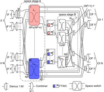
This section introduces the A-MF-SPIW architecture (Fig. 1) consideringN input/output interfaces (II/OIs), each pro-vided with F optical fibers carrying M wavelengths. The
N:1 Space switch space stage A Combiner Demux 1:M FTWC !1 1 M IF 1 IF 1 OF 1 NF r 1 r OF 1 NF space stage B IF F IF F OF F OF F 1 !M NWC:1 (NF+1):1 NFx(NF+r) 1 II 1 II N OI 1 OI N 1xN F 1 r 1xNF M M 2 NWC NF
Fig. 1. A-MF-SPIW architecture with N input/output interfaces equipped with F optical fibers carrying M wavelengths each. The switch is equipped with M pools of r < N F WCs dedicated per input wavelength. total number of channels per interface is NC = M F .
To solve contention in wavelength domain, the architec-ture is equipped with fixed-input/tunable-output Wavelength Converters (WCs) which are simpler and less expensive than tunable-input/tunable-output ones [6],[10]. WCs are partitioned in M pools of r < N F WCs each; each pool serves packets coming on the same wavelength, so WCs are shared-per-input-wavelength [7]. The total number of WCs is NW C = M r and their output range is M .
The architecture presented in Fig. 1 is now described in detail. In this architecture single-stage space switches are considered to connect IIs, OIs and WC pools. The archi-tecture is organized to minimize the complexity in terms of Optical Gates (OGs) using such single-stage switches. OGs can be implemented for example by using Semiconductor Optical Amplifiers (SOAs), microring resonators, acousto-optical devices and so on. After wavelength demultiplexing, channels related to the same wavelength on the different input fibers (N F ) are connected to a space switch dedi-cated to that wavelength. The input fibers are connected to the space switches according to a shuffle permutation. Packets arriving at a space switch can be either directly forwarded to one of the N F output fibers or forwarded to the corresponding pool ofr WCs. In this first space stage A, there areM space switches of size N F × (N F + r). After
the WC stage, each WC is connected to a 1 × N F space
switch needed to connect it to the proper output fiber. In
this space stage B, there areNW C = M r space switches.
A set ofN F combiners NW C : 1, each connected to one
of the output fibers, is used to multiplex the signals coming
from the NW C WCs. The NW C space switches and the
N F combiners are interconnected according to a shuffle permutation, so that each WC is connected to all combiners, and vice-versa. Finally, at the output fibersN F combiners (N F + 1) : 1 are used to multiplex the signals coming from the input fibers (up toN F ) and the signals coming from the WC pools. Neglecting the signals coming from the WCs, the signals from the input fibers are connected to the combiners according to a shuffle permutation.
The proposed architecture is equipped with multi-fiber interfaces; this kind of architecture is able to forward up toF packets coming on the same wavelength to the same OI (one packet per fiber), thus partially solving contention among packets on the same wavelength. In the single-fiber case (F = 1), instead, only one packet per wavelength can be forwarded to the same OI. Assuming the number of channels per interfaceNC = M F as a constant value, the
higher the number of fibers per interface (denoted byF ), the better the packet loss performance even with no wavelength conversion. Furthermore, when wavelength conversion is considered, increasing F allows to reduce the number of WCs needed in the architecture (contention partially solved by multi-fiber solution) and also to reduce the range of each WC (M F constant, if F increases M decreases). This aspect will be further evidenced in Sec. IV.
On the other hand, increasing the number of fibers means also increasing the complexity of the architecture in terms of optical devices. So the best trade-off should be found to obtain desired performance with minimum complexity.
The complexity of the A-MF-SPIW architecture can be evaluated taking into account that the space stage A needs M single-stage space switches of size N F ×(N F +r) while the space stage B needsNW C single-stage space switches
of size1 × N F . After some math (remembering that NC=
M F and NW C = M r) the complexity can be expressed as
NOG= N2F NC+ 2N F NW C. (1)
Considering the first term, the complexity increases linearly withF . In the second term, the complexity increases linearly with F if the total number of WCs NW C is fixed. It is
anyway important to emphasize thatNW C decreases as F
increases (see Sec. IV), so the dependence of the second term onF needs to be carefully evaluated.
A qualitative analysis of the complexity can be described as follows: in the space stage A, the size of each space switch increases as(N F )2+ N F r = F2(N2+ N
NCNW C), but the number of space switches (M = NC
F ) is in inverse
relation withF . In the space stage B, the size of each space switch increases as N F , and the number of space switches is related toNW C, which decreases asF increases.
The architecture is operated in an asynchronous scenario, where a packet is scheduled as it arrives at the input
interface. When a packet arrives at the switch on wavelength w, the scheduling algorithm randomly selects one fiber (say f ) on the destination interface for which wavelength w is available and then the packet is forwarded to wavelength w of fiber f . If all the wavelength channels related to w are busy on the destination interface then the outgoing wavelength (say g) is selected randomly among the ones that are free on at least one fiber of the destination interface. One of such output fibers (sayh) is randomly selected and the packet is forwarded on wavelength g of fiber h using one of the WCs in the pool dedicated to the incoming wavelengthw. A packet is lost either when all NCchannels
on the destination interface are busy at the time the packet arrives or when the arriving packet requires conversion and all r WCs dedicated to wavelength w are busy. More complex scheduling policies are left for future research. The analytical model presented in Sec. III is developed taking the scheduling procedure described above into account.
III. ANALYTICALMODEL OFA-MF-SPW
In the proposed model, the traffic destined to OI n (n = 1, . . . , N ), is assumed to be a Poisson process with intensity λ. The total packet arrival rate to the switch is then N λ. We also assume that the wavelength of an incoming optical packet is assumed to be uniformly distributed over the M wavelengths. Packet lengths are assumed to be exponentially distributed with mean set to unity and therefore the time unit in this article is set to the mean packet length. More general traffic patterns in which different OIs receive different intensities of traffic are left for future research. The load per input channel is denoted byp = λ
M F = λ NC.
Let us now focus on a tagged OIn whose statistical nature is the same as the other OIs. Let L(t) denote the number of occupied wavelength channels for OI n at time t. The processL(t) ∈ {0, 1, . . . , NC} is not a Markov process but
under some assumptions (which will be clarified later on), it can be approximated by a Markov process. For this purpose, we have the following two assumptions:
• WhenL(t) = i, the probability that an arriving packet
requires conversion is pi (i = 0, 1, . . . , NC− 1). • Given that a packet requires conversion, the probability
of this packet to find all converters busy in its as-sociated pool is given by pB and this probability is
independent from the processL(t).
Under these two assumptions, the random processL(t) can be shown to be a non-homogeneous birth-death (BD) type Markov chain. The birth rate ηi of this chain at statei (the
transition rate from state i to i + 1) is then given by ηi= λ(1 − pi) + λpi(1 − pB), i = 0, . . . , NC− 1, (2)
The death rate at statei is denoted by µi= i (transition rate
from statei to i − 1) due to exponential packet lengths with parameter one. If the probabilitiespi andpB were known,
then we could find the steady-state probabilities πi (i =
0, 1, . . . , NC) of this Markov chain which actually is the
steady-state probability that the Markov chain corresponding to OIn is visiting state i. Because of the “Poisson arrivals see time averages” property the packet loss probability (PLP) for a packet directed to OIn can be expressed as
P LP = πNC +
NXC−1
i=1
πipipB, (3)
The first term amounts to the case when an arriving packet finds all NC wavelength channels occupied. On the other
hand, the second term considers the case when there are idle channels on the OI but the packet requires conversion and is dropped due to the lack of a suitable WC.
However, the quantitiespB andpiare not known yet. For
the former quantity, the intensity of the traffic destined to OIn requiring conversion is given by
ν =
NXC−1
i=1
λπipi. (4)
The intensity of the overall traffic destined to the WC pool dedicated to a particular wavelength w is N ν
M . There are
indeedN OIs and the overall traffic is uniformly distributed amongM WC pools. Under the assumption that this traffic is Poisson, the quantitypBcan be obtained using the
Erlang-B formula corresponding to the case of r servers fed with Poisson traffic with utilization N νM.
Next, we describe how we approximate the quantitypifor
i = 1, . . . , NC− 1. For the purpose of approximating the
quantitypi, we first assume no wavelength conversion, i.e.,
r = 0. In this case for the designated OI n we have M server groups each one withF servers and fed with Poisson traffic with intensity Mλ. Due to the lack of WCs, server groups are independent from each other and the steady-state occupancy probabilities of each server group can be found from the M/M/F/F queue formalism. Let xj denote the steady-state
probability of j channels being occupied for OI n when r = 0. Note that the probabilities xjs can be found on
the basis of the steady-state distribution of an individual M/M/F/F queue but a detailed description of their efficient calculation is omitted in this paper due to space limitations. Now, consider the following birth-death processX(t) with death rate at statej µj= j and birth rate βj
βj = xj+1µj+1 xj =xj+1(j + 1) xj , j = 0, 1, . . . , NC− 1. (5) It is clear from the global balance equations of this Markov chain that xj is the steady-state probability
limt→∞P (X(t) = j). When r = 0, although a
one-dimensional Markov chain does not suffice to represent the system behavior, the one-dimensional Markov chain constructed above using xj has the correct steady-state
probabilitiesxj and therefore can be used to approximate
system behavior whenr = 0. We propose in this article to choosepisuch that the birth rates of the two Markov chains
and thus pB = 1. By comparing (2) and (5) with pB = 1
we can write λ(1 − pi) = βi or equivalently
pi= 1 −
βi
λ, i = 0, 1, . . . , NC− 1. (6) We have shown that choosing pi in this way allows one
to use a one-dimensional Markov chain L(t) or X(t) to correctly find the loss probabilities for the caser = 0.
For the caser > 0, it is worth noting that the probability that a packet requires wavelength conversion is independent from the number of WCs available and the particular sharing scheme adopted which indeed only affects the packet loss due to lack of WC (pB). So the conversion probabilitiespi
should not be sensitive to the particular value ofr and they can be maintained also in the case r > 0. To summarize the whole fixed-point procedure, an arbitrary pB is first
considered to construct the Markov chain L(t) using pis
as given in (6). The Markov chain is then solved to find probabilities πi and the probabilitypB is re-calculated for
an r-server system fed with Poisson traffic with intensity N ν/M where ν is defined as in (4). This procedure is then repeated until convergence, i.e. until two successive values forpB are as close to each other as desired. Finally (after
convergence) the expression (3) is used to evaluate PLP.
IV. NUMERICALRESULTS
This section presents model validation and a set of results related to PLP and complexity of the A-MF-SPIW switch. To validate the analytical model, analysis is compared against simulation results obtained by applying the random scheduling procedure described in Sec. II to Poisson arrivals. Simulation results have been obtained with confidence in-terval equal to or less than 10% of the average loss, with 95% probability. To make the relationship between the loss probability and the number of WCs clear in the figures, the conversion ratio α = NW C
N NC =
r
N F is here introduced.
α normalizes the total number of WCs with respect to its maximum valueN NC. The range of values forα is between
0 (no conversion case) and 1 (one WC per input channel). It is worthwhile noting that only some discrete values are allowed for α, indeed every time a WC per wavelength is added,r increase of 1 unit, while NW C increases ofM .
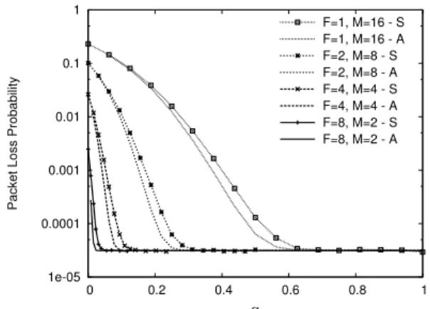
Figure 2 depicts the PLP as a function of the conversion ratio α, for analysis (A) and simulation (S) for the case
N = 16, NC = M F = 16 and p = 0.3. The number
of fibers per interface varies as F = 1, 2, 4, 8 and the
parameter M changes accordingly. The figure shows how
analytical results perform close to the simulation, even if the model underestimates PLP. The model captures the the trend of the curves in the region where the number of WCs is limited, which is not trivial in the multi-fiber case. The model also perfectly captures the asymptotic value of PLP, which is related to the loss due to output blocking on the output fibers and only depends (under the same load condition) on the total number of channels NC (kept
1e-05 0.0001 0.001 0.01 0.1 1 0 0.2 0.4 0.6 0.8 1
Packet Loss Probability
α F=1, M=16 - S F=1, M=16 - A F=2, M=8 - S F=2, M=8 - A F=4, M=4 - S F=4, M=4 - A F=8, M=2 - S F=8, M=2 - A
Fig. 2. PLP as a function of the conversion ratio α for analysis (A) and
simulation (S). PLP is shown as in the case N= 16, NC= M F = 16,
p= 0.3 and F varying from 1 to 8.
constant here). As a matter of fact, PLP modeling when F increases is a non-trivial problem due to the correlations among packets, especially in the current case where WCs are partitioned among the wavelengths. The proposed model maintains an adequate level of accuracy for all values of F allowing to identify the numberαthof WCs needed to reach
asymptotic performance. The figure shows thatαthrapidly
decreases whenF increases, due to the reuse of wavelengths in different fibers as explained in II.
Having verified that the model produces good results even for highF , the effect of other parameters (p, NC,N ) on the
accuracy of the model will now be evaluated. Fig. 3 depicts the PLP as a function of α, for the case N = 16, F = 2, M = 8, and varying the load as p = 0.2, 0.3, 0.5, 0.7. The
1e-07 1e-06 1e-05 0.0001 0.001 0.01 0.1 1 0 0.2 0.4 0.6 0.8 1
Packet Loss Probability
α p=0.7 - S p=0.7 - A p=0.5 - S p=0.5 - A p=0.3 - S p=0.3 - A p=0.2 - S p=0.2 - A
Fig. 3. PLP as a function of the conversion ratio α for analysis (A) and
simulation (S). PLP is shown as in the case N = 16, NC = M F = 16
(F = 2, M = 8) varying load (p = 0.2, 0.3, 0.5, 0.7).
accuracy of the model is very good when the load is high, due to the high loss related to blocking, which shadows the approximation introduced in the evaluation of the loss on WC pools. When the load decreases, the underestimation provided by the model increases, even if the minimum number of WCs needed for asymptotic performance can be
evaluated using the model with good accuracy (recall that α is a discrete value). This trend as a function of load is present in all switch configurations.
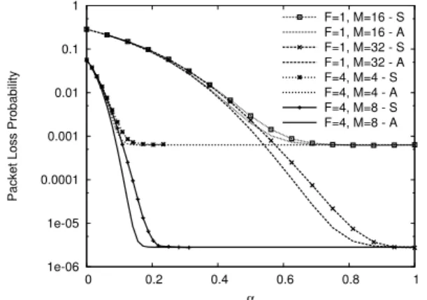
Fig. 4 presents further comparison between analysis and simulations by varyingNCbut with fixedN , for the scenario
N = 16, NC= 16, 32 and p = 0.4. In particular, the cases
(F = 1, M = 16), (F = 4, M = 4) and (F = 1, M = 32),
(F = 4, M = 8) are considered for NC = 16 and NC =
32, respectively. The model provides results closer to the
1e-06 1e-05 0.0001 0.001 0.01 0.1 1 0 0.2 0.4 0.6 0.8 1
Packet Loss Probability
α F=1, M=16 - S F=1, M=16 - A F=1, M=32 - S F=1, M=32 - A F=4, M=4 - S F=4, M=4 - A F=4, M=8 - S F=4, M=8 - A
Fig. 4. PLP as a function of α for analysis (A) and simulation (S). PLP
is shown as in the case N = 16, NC = 16, 32 and p = 0.4. The cases
(F = 1, M = 16), (F = 4, M = 4) and (F = 1, M = 32), (F = 4,
M= 8) are considered for NC= 16, NC= 32, respectively.
simulation when NC is lower, due to the higher asymptotic
PLP (same effect as explained for previous figure). The discrepancy between analysis and simulation is in the same order of the one obtained in Fig. 2, in fact the asymptotic losses obtained in these cases are comparable. By observing Fig. 4, it is possible to extract peculiar information. For example whenNC increases the PLP rapidly decreases due
to statistical multiplexing gain. When the number of WCs is limited, PLP obtained with NC = 16, NC = 32 is the
same. This is due to the fact that in this case the loss in the WC pools dominates the overall loss; given that WCs are partitioned among the wavelengths, this loss is only related to the number of channels on the same wavelength, which is N F (see Fig. 1). As a matter of fact, there are the same number N F of input channels competing on the same wavelength when (F = 1, M = 16), (F = 1, M = 32) and when (F = 4, M = 4), (F = 4, M = 8). Only when the number of WCs increases enough, and the loss in the WC pools becomes negligible, the PLP moves to different asymptotic values, related to NC.
A final comparison varyingN with fixed NCis presented
in Fig. 5. The PLP is plotted forN = 8 and N = 20, consid-eringNC= 24 and in particular the cases (F = 1, M = 24),
(F = 4, M = 6). The figure highlights how the model is less precise when N is small, for both values of F . The model approximation is acceptable for N = 20, while for N = 8 the gap between analysis and simulation is notable.
1e-06 1e-05 0.0001 0.001 0.01 0.1 1 0 0.2 0.4 0.6 0.8 1
Packet Loss Probability
α N=8, F=1, M=24 - S N=8, F=1, M=24 - A N=20, F=1, M=24 - S N=20, F=1, M=24 - A N=8, F=4, M=6 - S N=8, F=4, M=6 - A N=20, F=4, M=6 - S N=20, F=4, M=6 - A
Fig. 5. PLP as a function of the conversion ratio α for analysis (A)
and simulation (S). PLP is shown as in the case N = 8, 20, NC = 24,
p= 0.3. For both N = 8 and N = 20 two cases are considered: (F = 1,
M= 24), (F = 4, M = 6).
This is due to the fact that for small N , individual fibers and WC pools become very correlated which is ignored in our analytical model. Therefore,N needs to be relatively large, i.e.,N ≥ 8, for such fixed-point approximations to hold and provide good results and accuracy is increased with increasing number of interfaces. Note that also the performance of the A-MF-SPIW switch improves for large N , as can be deduced from previous figure, due to the better sharing of WC pools with highN . Thus, the model performs better exactly in such configurations where the proposed architecture gives best performance.
To provide an example of switch dimensioning, Fig. 6 shows the total number of WCs needed to obtain the PLP lower than a certain value (1e-3, 1e-4, 1e-5, 1e-6) as a function ofF , as in the case N = 20, NC = 24, p = 0.3.
This value is indicated withNth
W C. Fig. 6 can be obtained
10 100 1 2 3 4 5 6 7 8 Number of WCs (N WC ) F N=20, Nc=24, PLP < 1e-6, - S N=20, Nc=24, PLP < 1e-6, - A N=20, Nc=24, PLP < 1e-4 - S N=20, Nc=24, PLP < 1e-4 - A
Fig. 6. Total number of WCs Nth
W Cneeded to obtain PLP lower than a
certain value (1e − 4, 1e − 6) as a function of F , as in the case N = 20,
NC= 24, p = 0.3. (A) stands for analysis and (S) for simulation.
by using Fig. 5 and similar and by taking into account that NW C = αN Nc. The figure shows values obtained using
both analysis and simulation. Nth
F increases, for both values of PLP. The error in switch dimensioning using analysis is quantified by the figure and it increases as F increase, due to the fact that with high F PLP rapidly decreases in the region whereNW C is low (see
Fig. 5). The figure gives an idea about the relative error with respect to the total number of WCs, which is low whenF is low, and then increases almost linearly. The model provides good estimation of Nth
W C when F is not very high, which
seems to be a reasonable trade-off in terms of complexity. Evaluation of switch complexity is provided in Tables I and II, which contain the values of αth, Nth
W C and NOG
needed to obtain PLP ≤ 1e-4 and 1e-6, respectively, as in
the case N = 20, NC = 24, p = 0.3. The number of WCs
Nth
W C is obtained from previous figure while OGs NOG is
obtained by applying formula (1), accordingly. Tables show values for different couples (F , M ) while keeping the total number of channel as a constant,NC= 24. The tables show
(F, M ) (1, 24) (2, 12) (4, 6) (6, 4) (8, 3) A αth 0.45 0.175 0.0625 0.025 0.0125 NW Cth 216 84 30 12 6 NOG 18240 25920 43200 60480 78720 S αth 0.45 0.2 0.075 0.03333 0.01875 NW Cth 216 96 36 16 9 NOG 18240 26880 44160 61440 79680 TABLE I
VALUES OFαth, NW Cth , NOGNEEDED TO OBTAINPLP ≤ 1E-4AS IN
THE CASEN= 20, NC= 24, p = 0.3FOR DIFFERENT(F , M ).
(F, M ) (1, 24) (2, 12) (4, 6) (6, 4) (8, 3) A αth 0.6 0.25 0.0875 0.041667 0.025 NW Cth 288 120 42 20 12 NOG 21120 28800 45120 62400 80640 S αth 0.65 0.3 0.125 0.06667 0.04375 NW Cth 312 144 60 32 21 NOG 22080 30720 48000 65280 83520 TABLE II
VALUES OFαth, NW Cth , NOGNEEDED TO OBTAINPLP ≤ 1E-6AS IN
THE CASEN= 20, NC= 24, p = 0.3FOR DIFFERENT(F , M ).
how the total number of WCs can be reduced substantially by increasing F . As an example, in Table I with F = 4 using simulation, α = 0.075, so the WC saving is equal to 92.5% with respect to a switch equipped with one WC per channel. In particular, every time F doubles, Nth
W C is
reduced by more than half. The price to pay to obtain this saving in WC is the increase of the number of OGs, which increases almost linearly with the number of fibers F , and the increase is comprised between 50%-75% every time F doubles. The number of OGs evaluated with simulation and analysis do not differ much, in fact whenF increases most of the complexity is related to the direct interconnection
of the input/output fibers, less to the connection of WCs. A trade-off among the number of WCs employed and the number of OGs need to be evaluated, thus choosing the proper value ofF . Further evaluations and comparisons with other switch architectures with wavelength converters can be straightforwardly obtained by applying formulas, similar to (1), reported, for example, in [10].
V. CONCLUSIONS
This paper presents an analytical model to evaluate packet loss in a shared per wavelength optical switch with multi-fiber interfaces. Besides filling a methodological gap regard-ing this kind of architecture and validatregard-ing the analytical approach against simulation, the paper produces useful numerical results regarding the wavelength converters saving achieved by the approach with asynchronous operation. The switch design process shall take into account also component availability and cost to achieve an overall switch cost optimization, including both wavelength converters and space switching subsystems.
REFERENCES
[1] S. J. Ben Yoo. ”Optical packet and burst switching technologies for the future photonic Internet”, IEEE J. Lightwave Technol., Vol. 24, pp. 4468-4492, Dec. 2006.
[2] M. J. OMahony, C. Politi, D. Klonidis, R. Nejabati, D. Simeonidou, ”Future Optical Networks”, IEEE J. Lightwave Technol., Vol. 24, Issue 12, pp. 4684-4696, Dec. 2006.
[3] K. Vlachos, C. Raffaelli, S. Aleksic, N. Andriolli, D. Apostolopoulos, H. Avramopoulos, D. Erasme, D. Klonidis, M. N. Petersen, M. Scaffardi, K. Schulze, M. Spiropoulou, S. Sygletos, I. Tomkos, C. Vazquez, O. Zouraraki, F. Neri, ”Photonics in switching: enabling technologies and subsystem design”, OSA J. Opt. Netw., Vol. 8, No. 5, pp. 404-428, May 2009.
[4] S. Yao, B. Mukherjee, S. J. Ben Yoo, S. Dixit, ”A Unified Study of Contention-Resolution Schemes in Optical Packet-Switched Net-works”, IEEE J. Lightwave Technol., Vol. 21, pp. 672-683, 2003. [5] N. Akar, C. Raffaelli, M. Savi, E. Karasan, ”Shared-per-wavelength
asynchronous optical packet switching: A comparative analysis”,
Com-puter Networks, vol. 54, no. 13, pp. 2166-2181, 2010.
[6] Y. Fukushima, H. Harai, S. Arakawa, M. Murata, ”Design of Wavelength-convertible Edge Nodes in Wavelength-routed Networks”,
J. Opt. Netw., Vol.5, No.3, pp.196-209, 2006.
[7] C. Raffaelli, M. Savi, A. Stavdas, ”Multistage Shared-per-Wavelength Optical Packet Switch: Heuristic Scheduling Algorithm and Perfor-mance”, IEEE J. Lightwave Technol., Vol. 27, Issue 5, pp. 538-551, March 2009.
[8] C. Raffaelli, M. Savi, G. Tartarini, D. Visani, ”Physical Path Analysis in Photonic Switches with Shared Wavelength Converters”, in pro-ceedings of ICTON 2010, Munich, Germany, June 27-July 1 2010, Mo.C1.5.
[9] C. Raffaelli, M. Savi, ”Power Consumption in Photonic Switches with Shared Wavelength Converters”, in proceedings of ICTON 2010, Munich, Germany, June 27-July 1 2010, We.B1.6.
[10] V. Eramo, A. Germoni, C. Raffaelli, M. Savi, ”Multifiber Shared-Per-Wavelength All-Optical Switching: Architecture, Control and Perfor-mance”, IEEE J. Lightwave Technol., Vol. 26, Issue 5, pp. 537-551, March 2008.
[11] C. Raffaelli, G. Muretto, ”Combining Contention Resolution Schemes in WDM Optical Packet Switches with Multifiber Interfaces”, OSA
Journal of Optical Networking, special issue on Photonics in Switch-ing, Vol. 6, N. 1, January 2007, page. 74-89, USA.
[12] V. Eramo, A.Germoni, A. Cianfrani, M. Listanti, C. Raffaelli, ”Eval-uation of Power Consumption in Low Spatial Complexity Optical Switching Fabrics”, IEEE Journal of Selected Topics in Quantum Electronics, 2010.