ANALYSIS OF TWO TYPES OF CYCLIC
BIOLOGICAL SYSTEM MODELS WITH TIME
DELAYS
a thesis
submitted to the department of electrical and
electronics engineering
and the graduate school of engineering and science
of bilkent university
in partial fulfillment of the requirements
for the degree of
master of science
By
Mehmet Eren Ahsen
July 2011
I certify that I have read this thesis and that in my opinion it is fully adequate, in scope and in quality, as a thesis for the degree of Master of Science.
Prof. Dr. Hitay ¨Ozbay(Supervisor)
I certify that I have read this thesis and that in my opinion it is fully adequate, in scope and in quality, as a thesis for the degree of Master of Science.
Prof. Dr. ¨Omer Morg¨ul
I certify that I have read this thesis and that in my opinion it is fully adequate, in scope and in quality, as a thesis for the degree of Master of Science.
Assoc. Prof. Dr. Co¸sku Kasnako˘glu
Approved for the Graduate School of Engineering and Science:
Prof. Dr. Levent Onural
ABSTRACT
ANALYSIS OF TWO TYPES OF CYCLIC
BIOLOGICAL SYSTEM MODELS WITH TIME
DELAYS
Mehmet Eren Ahsen
M.S. in Electrical and Electronics Engineering
Supervisor: Prof. Dr. Hitay ¨
Ozbay
July 2011
In this thesis, we perform the stability analysis of two types of cyclic biologi-cal processes involving time delays. We analyze the genetic regulatory network having nonlinearities with negative Schwarzian derivatives. Using preliminary results on Schwarzian derivatives, we present necessary conditions implying the global stability and existence of periodic solutions regarding the genetic regu-latory network. We also analyze homogenous genetic reguregu-latory network and prove some stability conditions which only depend on the parameters of the non-linearity function. In the thesis, we also perform a local stability analysis of a dynamical model of erythropoiesis which is another type of cyclic system in-volving time delay. We prove that the system has a unique fixed point which is locally stable if the time delay is less than a certain critical value, which is analytically computed from the parameters of the model. By the help of sim-ulations, existence of periodic solutions are shown for delays greater than this critical value.
Keywords: Stability Analysis, Periodic Solutions, Monotone Dynamical System, Schwarzian Derivatives, Gene Regulatory Networks, Erythropoiesis, Poincar´e Bendixson Theorem, Hill Functions, Time Delay.
¨
OZET
ZAMAN GEC˙IKMEL˙I ˙IK˙I D ¨
ON ¨
US
¸SEL B˙IYOLOJ˙IK S˙ISTEM
MODEL˙IN˙IN ANAL˙IZ˙I
Mehmet Eren Ahsen
Elektrik ve Elektronik M¨
uhendisli¯
gi B¨
ol¨
um¨
u Y¨
uksek Lisans
Tez Y¨
oneticisi: Prof. Dr. Hitay ¨
Ozbay
Temmuz 2011
Bu tezde zaman gecikmeli iki farklı biyolojik sistem modelinin kararlılık analizi yapılmı¸stır. Zaman gecikmesi i¸ceren gen d¨uzenleyici sistem modelinin kararlılık analizi yapılmı¸stır. Bu modelde do˘grusal olmayan ¨o˘gelerin negatif Schwarz t¨urevleri oldu˘gu varsayılmı¸stır. Schwarz t¨urevleri hakkında elde edilen sonu¸clar kullanılarak, gen d¨uzenleyici sistem modelinin kararlılı˘gıyla ilgili sonu¸clar is-patlanmı¸stır. Ayrıca periyodik ¸c¨oz¨umlerin olu¸smasını sa˘glayan ko¸sullar elde edilmi¸stir. Homojen gen d¨uzenleyici sistem modeli incelenip kararlılı˘gıyla ilgili sonu¸clar bulunmu¸stur. Ayrıca zaman gecikmesi i¸ceren do˘grusal olmayan Er-itropoez modelinin kararlılık analizi yapılmı¸stır. ˙Ilk ¨once belirtilen sistemin tek bir denge noktası oldu˘gu ispatlanmı¸s, daha sonra sistem bulunan denge noktası etrafında do˘grusalla¸stırılmı¸stır. Sistemin gecikme de˘geri belli bir kritik de˘gerin altında olması ko¸suluyla yerel kararlı oldu˘gu g¨osterilmi¸stir. Simulasyonlar gecik-menin bu kritik de˘gerden y¨uksek oldu˘gunda periyodik ¸c¨oz¨umler ¨uretmi¸stir.
Anahtar Kelimeler: Kararlılık Analizi, Monoton Dinamik Sistemler, Schwarz T¨urevi, Gen D¨uzenleyici Sistemler, Poincar´e Bendixson Teoremi, Hill Fonksiy-onları, Eritropoez, Zaman Gecikmesi.
ACKNOWLEDGMENTS
I would like to express my deep gratitude to my supervisor Prof. Dr. Hitay ¨
Ozbay for his unlimited support, patience and guidance. I benefited a lot from his deep knowledge on the topics discussed in this work.
I would like to thank Prof. Dr. ¨Omer Morg¨ul and Assist. Prof. Co¸sku Kas-nako˘glu for reading and commenting on this thesis and for being on my thesis committee.
I would also like to express my deep gratitude to Dr. Silviu-lulian Niculescu, my co-advisor in the Bosphorus project, for his inspiring ideas and guidance.
Contents
1 Introduction 1
1.1 Cyclic Biological Processes . . . 1
1.2 Literature Review . . . 4
2 Preliminary Results 6 2.1 Definitions and Notations . . . 6
2.2 Linear Time Invariant Systems . . . 7
2.3 Functional Differential Equations . . . 14
2.4 Schwarzian Derivatives . . . 16
2.5 Fixed Points . . . 20
3 Gene Regulatory Networks 36 3.1 Problem Formulation . . . 36
3.2 Analysis of the Gene Regulatory Network . . . 39
3.2.2 Homogeneous Gene Regulatory Network with Hill Functions 50
3.2.3 Gene Regulatory System under Positive Feedback . . . 53
3.2.4 Homogenous Gene Regulatory Network under Positive Feedback . . . 55
3.3 Simulation Results . . . 63
4 A model of erythropoiesis 71
4.1 Erythropoiesis . . . 71
4.2 Mathematical Model for Erythropoiesis . . . 73
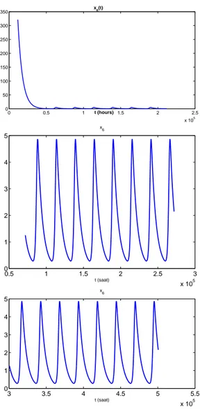
4.3 Simulation Results . . . 84
5 Conclusions 89
APPENDIX 91
A Erythropoiesis Model 91
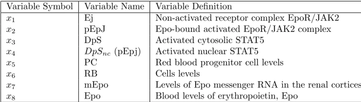
A.1 Model Variables . . . 91
A.2 Model Parameters . . . 92
List of Figures
2.1 A typical x vs h′(x) graph for type A function. . . . 28
2.2 A typical x vs h′(x) graph for type B function. . . . 29
3.1 A continuous time model of Gene Regulatory System . . . 37
3.2 x1(t), x2(t) and x3(t) vs t graphs of system with x(0) =
(1, 0.9, 0.8), τ = 0 . . . . 63
3.3 x1(t), x2(t) and x3(t) vs t graphs of system with x(0) =
(0.4, 2, 0.6), τ = 4 . . . . 64
3.4 x1(t), x2(t) and x3(t) vs t graph of system with x(0) = (3, 3, 4), τ = 0 65
3.5 x1(t), x2(t) and x3(t) vs t graphs of system with x(0) =
(0.3, 2, 3), τ = 0 . . . . 65
3.6 x1(t), x2(t) and x3(t) vs t graphs of system with x(0) =
(0.1, 2, 0.4), τ = 1 . . . . 66
3.7 x1(t), x2(t) and x3(t) vs t graphs of system with x(0) =
(3, 0.5, 1.5), τ = 5 . . . . 66
3.8 x1(t), x2(t) and x3(t), τ = 0 vs t graph for the homogenous gene
3.9 x1(t), x2(t), x3(t) and τ = 2 vs t graph with x(0) =
(0.9, 0.95, 0.85), τ = 0 . . . 67
3.10 x1(t), x2(t) and x3(t) vs t graph with x(0) = (5, 3, 0.7), τ = 5 . . . 68
3.11 x1(t), x2(t) and x3(t) vs t graph with x(0) = (3, 0.5, 4), τ = 0 . . . 68
3.12 x1(t), x2(t) and x3(t) vs t graph with x(0) = (1, 1.2, 1.4), τ = 0 . . 69
3.13 x1(t), x2(t) and x3(t) vs t graph with x(0) = (1, 1.2, 1.4), τ = 0 . . 70
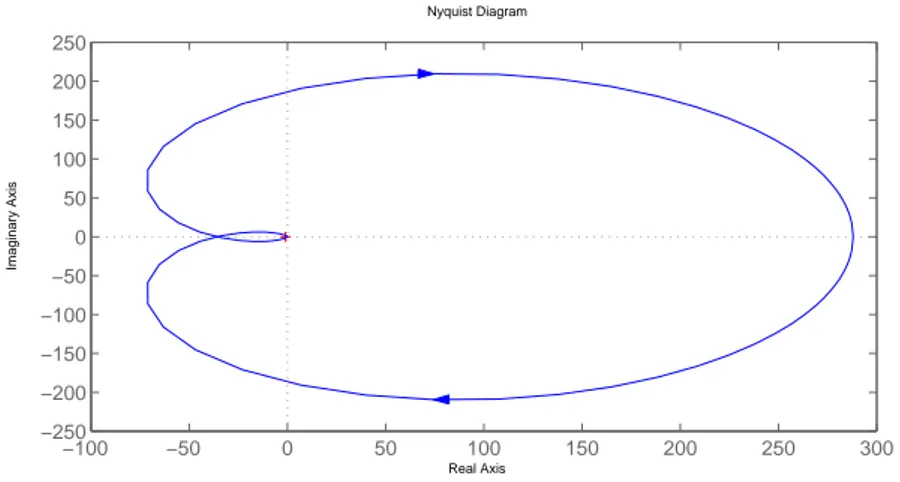
3.14 Nyquist Diagram of of G0(s) . . . . 70
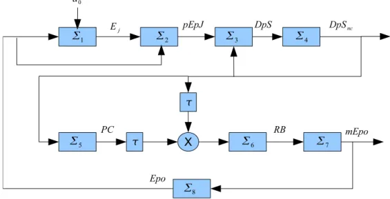
4.1 The feedback loop involved in the process of Erythropoiesis. . . . 72
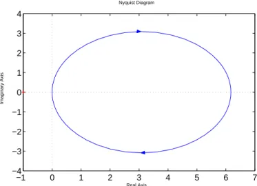
4.2 Nyquist Plot of the function KG(s). . . . 85
4.3 Bode plot of the function KG(s). . . . 85
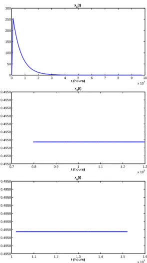
4.4 Output of the sixth coordinate x6 with initial conditions y and
τ = 1000h. . . . 86
4.5 Output of the sixth coordinate x6 with initial conditions yν and
List of Tables
A.1 Model variables of Erythropoiesis . . . 91
Chapter 1
Introduction
1.1
Cyclic Biological Processes
The process of creating images of the human body is called medical imaging. Af-ter Wilhelm Conrad R¨ontgen discovered X-Rays in 1895, they have been widely used for the purpose of creating various images of the human body. Although there are side effects due to exposure to radiation, medical imaging has saved thousands of lives by early diagnosis of disease. Creating machines for medical imaging purposes not only requires medical knowledge but also requires advanced knowledge of engineering and physics. This lead to the birth of a new interdisci-plinary field called Biomedical Engineering, which also deals with mathematical modeling of biological processes.
Since 1970s various models have been introduced for many different biological processes. Mathematical modeling of biological processes not only helps us to understand the underlying mechanisms better, but it also gives us a way of controlling them. For example, an effective and reliable model of a disease may help us determine correct therapeutic actions, e.g. the right amount of drug, or delivery time of the drug. In 1965, Goodwin has put forward a low-order
dynamical system that became the milestone example of biochemical oscillatory networks under negative feedback [1]. In this thesis we deal with the analysis of two different biological systems (a) gene regulatory networks, and (b) formation of red blood cells in the human body (erythropoiesis).
By means of genes we pass our traits to our offspring. Gene expression is the process by which the gene information is converted. It has two main processes known as transcription and translation. In transcription, genes are copied into messenger RNA after which mRNA is decoded to make the corresponding pro-tein. The transcription process is effected by the activities of regulatory proteins. The combination of these processes and interactions between regulatory proteins and mRNA are referred as gene regulatory network. Gene regulatory networks may be used to control various functions of living organisms since they play a very important role in the process of protein synthesization. In the first part of this thesis we will consider gene regulatory networks, which have the following general mathematical model:
˙ p1(t) = −kp1p1(t) + fp1(gm(t− τgm)) ˙g1(t) = −kg1g1(t) + fg1(p1(t− τp1)) .. . ˙ pm(t) = −kpmpm(t) + fpm(gm−1(t− τgm−1)) ˙gm(t) = −kg1gm+ fgm(pm(t− τpm)), (1.1)
where pi and gi represent the concentrations of protein and mRNA respectively
and the constants ki represent the degradation rates for mRNAs and proteins.
This model has been first analyzed by Goodwin in [1]. It has a cyclic pattern which one can encounter in other fields of science as well. In [2], Townley et al. considered a model similar to (1.1). The early results regarding oscillatory behavior of the model (1.1) has been put forward by Hasting et al. [3]. These results have been generalized by Mallet-Paret in [4]. Their result basically says that the solution of the model (1.1) either converges to the equilibrium point
or it is a nonconstant periodic solution. Basically, their result rules out any chaotic behavior. Then, Allwright presented a simple condition regarding the global attractivity of the unique equilibrium point, [5]. By using the results presented in [4] and [5], we will try to make an analysis of the model (1.1). We will analyze the system (1.1) with nonlinearities having negative Schwarzian derivatives. The concept of Schwarzian derivatives has been widely used in the analysis of nonlinear difference equations [6] as well as in projective geometry [7]. We will show in Chapter 2 that functions with negative Schwarzian derivatives have very special forms. By using the results from Chapter 2, in Chapter 3 we will present conditions regarding the stability and existence of oscillatory behavior of the model (1.1).
In Chapter 4, we will consider another vital biological process namely ery-thropoiesis which is the process of production erythrocytes known as red blood cells. The red blood cells are responsible of transporting oxygen to our body tissues, which is needed for energy production in our cells. We will consider a recent model of Erythropoiesis proposed by Lai et al. in [8]. We will show that the system in [8] has a unique equilibrium point which is locally stable for some values of the delay. A global analysis of the model is still an open problem.
The models studied in Chapters 3 and 4 fall into the category of cyclic non-linear systems with time delays. Analysis of such systems have been investigated extensively in the literature [9], [10], [11] and [12]. There are various technique developed depending on the type of nonlinearity and interaction of the time delay with the nonlinearities. Here we use methods from [5], [4], [13] and [14] to ana-lyze gene regulatory networks and erythropoiesis. Both systems have a feedback mechanism so techniques from feedback stability analysis are also used.
1.2
Literature Review
Note that we can rewrite the model (1.1) as follows:
˙z1(t) = −λ1z1(t) + g1(z2(t− τ1))
˙z2(t) = −λ2z2(t) + g2(z3(t− τ2))
.. .
˙zn(t) = −λnzn(t) + gn(z1(t− τn)). (1.2)
If we do the following change of variables
xi(t) := zi(t− hi), hi = i
∑
k=1
(τk), (1.3)
we obtain the mathematical model (1.4) which is equivalent to (1.2):
˙x1(t) = −λ1x1(t) + g1(x2(t)) ˙x2(t) = −λ2x2(t) + g2(x3(t)) .. . ˙xn(t) = −λnxn(t) + gn(x1(t− τ)), (1.4) where τ = n ∑ k=1 (τk) = hn. (1.5)
In Chapter 3, we analyze the gene regulatory network (1.4) and present some results regarding its stability. In [15], Wang et al. analyzed a generalized version of the system (1.4) and by using the result of [4] they prove some conditions implying delay independent unstability of equilibrium points, for which case the system (1.4) has periodic solution for all positive values of the delay. In [10], Enciso considered the gene regulatory network (1.4) under negative feedback. He presented a global stability result by using the methods of [9], [16] and [17]. Moreover, by using a Hopf bifurcation approach he showed existence of periodic solutions for some cases. In [14], Muller et al. introduced a general model for repressilator and analyzed the model using the fact that Hill functions have
negative Schwarzian derivatives. In the present work, we first prove that bounded functions with negative Schwarzian derivatives can only have two special forms and they can have at most three fixed points. Then by using the results of [4] and [5], we get the same global stability result of [10]. Different from [10] we will prove results regarding the stability of the linearized system. We will show that if the linearized system is unstable then system (1.4) has periodic solutions. Moreover, we give upper and lower bounds for possible periodic solutions of the system (1.4) under negative feedback. We also consider the homogenous genetic regulatory network under negative feedback with nonlinearities in the form of Hill functions and prove a result regarding the global stability of the homogenous system. Furthermore, we analyzed the system (1.4) under positive feedback which is to the author’s knowledge has not been considered in the literature yet. We proved a global stability result regarding the positive feedback case by using the results presented in [18]. In [18], Smith makes a general analysis regarding the stability of monotone systems which includes the general regulatory network model we consider as a subcase. His results lead us conclude that the general solution of the system (1.4) under positive feedback converges towards an equilibrium point of it [18], [19]. We also analyzed the homogenous genetic regulatory network under positive feedback as a subcase.
In Chapter 4, we analyze the Erythropoiesis model proposed by Lai et al. in [8]. To the author’s knowledge the model has not been investigated in the literature. In the present work we prove a local stability result regarding the Erythropoiesis model. But the nonlinearities involved in the model does not possess special patterns which makes it hard to make a global analysis of the model.
Chapter 2
Preliminary Results
2.1
Definitions and Notations
In this section we will try to present some basic definitions and notations that are frequently used in the thesis. Although most of the results presented in this chapter can be generalized to any inner product space, we will concentrate on Rn equipped with the usual Euclidean norm defined as
||x|| =√x2
1+ ... + x2n, for x = (x1, ..., xn)T ∈ Rn. (2.1)
A subset K of the vector spaceRn over the fieldR is called a convex cone if for
any scalars α , β ∈ R+ and vectors x, y∈ K we have
αx + βy ∈ K. (2.2)
Since the biological parameters such as number of genes, enzymes, mRNA take positive values, we will analyze our systems in the cone Rn
+ which is defined as
Rn
+ ={x ∈ R
n: x
i ≥ 0 ∀i = 1, 2, ..., n}. (2.3)
The symbol C will denote the set of complex numbers and the set C+ is defined
as
For a function
g(x) : K → K, (2.5)
where K is any set, gn(x) will denote the function which is the composition of
g(x) with itself n times. Given an interval I ⊆ R, Dn(I) will denote the set of n times continuously differentiable functions defined on the interval I. A function f (x) defined from the normed linear space X to the normed linear space Y is bounded if
∃M ≥ 0 such that ||f(x)||Y ≤ M||x||X ∀x ∈ X. (2.6)
A complex valued function f is said to belong to the set H∞ if it is analytic and bounded in C+. The set H∞ is a commutative ring with unity over itself [13].
For a function f ∈ H∞, the infinity norm of f denoted as ||.||∞ is defined as follows:
||f||∞ = ess sup s∈C+
|f(s)|. (2.7)
Note that this definition makes sense since f is bounded and analytic in C+.
Let x(t) be a vector function depending on the variable t. A point y ∈ Rnis said to be an omega point of x(t) if there is an increasing sequence 0 < ti → ∞ and
we have
lim
ti→∞
(x(ti)) = y.
The omega limit set of the solution x(t) is the set of omega points of x(t).
2.2
Linear Time Invariant Systems
Linear systems are commonly encountered in engineering, mathematics and eco-nomics. This chapter will present some basic results from Linear System Theory that will be used frequently in Chapters 3 and 4 of the thesis. A retarded linear time invariant (LTI) system with a single delay has the following state space
representation:
˙x(t) = A0x(t) + A1x(t− τ), τ > 0, (2.8)
where A0, A1 ∈ Rn×n and x(t) ∈ Rn. Although the results we have in this
section can easily be generated to multiple delay case, we will concentrate on single delay case as the mathematical models we will analyze in Chapters 3 and 4 have single delays.
Definition 1. The characteristic function χ(s) associated with the system (2.8) is given by
χ(s) = det(sI− A0− A1e−τs). (2.9)
Definition 2. The characteristic function (2.9) is said to be stable if
χ(s)̸= 0, ∀s ∈ C+. (2.10)
The system (2.8) is said to be stable if its characteristic function is stable. The system (2.8) is said to be stable independent of delay if it is stable for all τ ≥ 0.
For constant matrices A0, A1, the characteristic equation of the system (2.8)
will be in the following form:
χ(s) = p0(s) + p1(s)e−τs= 0, (2.11)
where p0(s), p1(s) are polynomials of degree n and n− 1 respectively.
Notice that when p0(s) and p1(s) in (2.11) do not have a common zero inC+,
we have
χ(s0) = 0 for some s0 ∈ C+ ⇔ 1 +
p1(s0)e−τs0
p0(s0)
= 0. (2.12)
We will now present a Lemma which is commonly known as the Small-Gain Theorem.
Lemma 1. Let g(s), h(s)∈ H∞ such that ||gh||∞ < 1.
Then, the characteristic function
χ(s) = 1 + g(s)h(s)e−τs
is stable for all τ ≥ 0.
Proof. For fixed τ , we know that the characteristic function
χ(s) = 1 + g(s)h(s)e−τs
is stable if
χ(s)̸= 0, ∀s ∈ C+.
Suppose for some s0 ∈ C+, we have
χ(s0) = 1 + g(s0)h(s0)e−τs0 = 0
⇒ g(s0)h(s0)e−τs0 =−1
⇒ |g(s0)h(s0)| ≥ 1
⇒ ||gh||∞≥ 1,
which contradicts the fact that||gh||∞ < 1.
As a corollary of Lemma 1, we have the following result.
Lemma 2. Let G∈ H∞, then for all |k| < ||g||−1∞ the characteristic equation
χ(s) = 1 + kG(s)e−τs (2.13)
is stable independent of delay.
Proof. Let h(s) = k, then we have
||Gh||∞ < 1
Consider a characteristic function of the form (2.13), then ωc > 0 is called a
gain crossover frequency of the characteristic equation if we have
|kG(jωc)| = 1. (2.14)
Similarly, we call ωg a phase crossover frequency of the characteristic equation if
cos(∠k + ∠G(jωg)) = −1. (2.15)
Let us now analyze a characteristic function of the following form:
χ(s) = 1 + ke
−τs
(s + a1)...(s + an)
= 0 k ∈ R, ai ∈ R+. (2.16)
We will now present a Lemma regarding the stability of a characteristic equation in the form (2.16). The proof of the Lemma will require the famous Nyquist criteria in control theory. One may check [20] or any other introductory material on control theory for a proof of the Nyquist result. Basically, Nyquist criteria says that the characteristic equation (2.16) is stable if its Nyquist plot does not encircle the point−1.
Lemma 3. Consider a characteristic equation in the form (2.16) and let Kl=
n
∏
i=1
(ai). (2.17)
Then one of the following holds:
1. If 0 < k < Kl, then χ(s) is stable independent of delay.
2. If Kl≤ k ≤ Ku, then χ(s) is stable ∀τ < τm and unstable ∀τ ≥ τm, where
τm is smallest positive number satisfying
τ = 1 ωc ( 2πh + π− n ∑ i=1 arctan(ωc ai ) ) , h∈ Z
where ωc > 0 is the unique gain crossover frequency satisfying the following
equation:
n
∏
and Ku is given by the following formula Ku = v u u t∏n i=1 (ω2 g+ a2i),
where ωg > 0 is the smallest ω satisfying
cos ( n ∏ i=1 ( arctan ( ω ai ))) =−1. 3. If k≥ Ku, then χ(s) is unstable independent of delay.
4. If−Kl < k < 0, then χ(s) is stable independent of delay.
5. If k≤ −Kl, then χ(s) is unstable independent of delay.
Proof. For fixed ai ∈ R+, let χ(s) be a characteristic equation in the form (2.16).
We have ke−τjωc (jωc+ a1)...(jωc+ an) = 1 ⇔ n ∏ i=1 (ω2c + a2i) = k2. But h(ω) =∏ni=1(ω2+ a2
i) is an increasing function of ω and
h(0) =
n
∏
i=1
(a2i), h(∞) = ∞. Therefore if k≥ Kl, we have unique ωc satisfying
n ∏ i=1 (ω2c + a2i) = k2. Let Gτ(s) be defined as Gτ(s) = e−τs ∏n i=1(s + ai) .
If k satisfies the condition given in Part 1 and 4, then we ||kGτ(s)||∞ < 1 ∀τ ≥ 0
and the result follows from Lemma 2. For the proof of part 2 and 3, suppose that we have k ≥ n ∏ i=1 (ai) = Kl
and consider the delay free system
f (s) = 1 + kG0(s). (2.18)
Since the roots of the characteristic function f (s) depends continuously on the parameter k, we conclude that f (s) is stable for all k < Ku where Ku is the
smallest positive number such that the characteristic equation
1 + KuG(s) = 0 (2.19)
has a root on the imaginary axis [21]. That is ∃ ωg > 0 such that
1 + KuG0(jωg) = 0 ⇒ Ku =− n ∏ i=1 (jωg + ai) ⇒ Ku = v u u t∏n i=1 (w2 g+ a2i),
where ωg is the smallest positive number satisfying
cos ( n ∏ i=1 ( arctan ( ωg ai ))) =−1. If k≥ Ku then we have kG0(jωg)≤ −1
so the Nyquist plot of the delay free system encircles the point−1 and the delay free system is unstable by Nyquist criteria. Hence, if we have
Kl ≤ k ≤ Kp
then the delay free system is stable. By the continuous dependence of the roots on the parameter τ , we know that the system will be stable for all τ < τm where
at τm is the smallest positive number such that for τ = τm the characteristic
function χ(s) has a root on the imaginary axis [21]. That is∃ ωc ≥ 0 satisfying
1 + ke
−jτmωc
∏n
i=1(jωc + ai)
where ωc is the unique frequency satisfying n
∏
i=1
(ωc2+ a2i) = k2
and τm is the smallest positive number satisfying
τm = 1 ωc ( 2πh + π− n ∑ i=1 arctan(ωc ai ) ) , for some h∈ Z. Note that τm depends on k and we have
τm(Ku) = 0 τm(Kl) = ∞. (2.20) If τ ≥ τm, we have ∠(ke−τjωcG(jω c)) <−π (2.21) since both τ ω, n ∑ i=1 arctan(ω ai ) (2.22)
are increasing functions of ω. But (2.21) and (2.22) implies that for τ ≥ τm the
Nyquist plot of χ(s) will encircle the point−1 more than once so χ(s) is unstable for τ ≥ τm. For part 3 of the Lemma, we have shown that if
k ≥ Kp,
then the delay free characteristic function is unstable and with the same argu-ments as part 2 of the Lemma, the characteristic function will remain unstable as we increase delay. For the proof of part 5 of the Lemma, note that for k≤ −Kl
and any positive delay we have
χ(0)≤ 0, χ(∞) = 1 ∀τ ≥ 0. Intermediate theorem implies that ∃ y ∈ R+ such that
χ(y) = 0 ∀τ ∈ R+. (2.23)
Equation (2.23) proves that the characteristic function is unstable independent of delay.
Although the systems we will consider in Chapters 3 and 4 are nonlinear, we need Lemma 3 to determine the stability of the linearized systems. We will use the fact that the linearized system and nonlinear system have similar local behavior around the vicinity of an equilibrium point of the nonlinear system.
2.3
Functional Differential Equations
Most of the processes we observe in the nature can not be accurately modeled by means of linear systems. Some processes involve nonlinearities, other processes involve both nonlinearities and time delays at the same time. Such systems are modeled by the help of functional differential equations. The biological systems we will consider in Chapters 3 and 4 are nonlinear and also have lumped delays. Therefore, we need to present some results that are widely used in the analysis of Functional Differential Equations. A general model for a nonlinear process is given by
˙x = f (t, x(t), x(t− τ)), t ∈ R+, x(t)∈ Rn, f :Rn→ Rn. (2.24)
Most of the physical systems that are modeled are casual. Therefore, we assume in (2.24) that
τ ≥ 0. (2.25)
If the function f (t, x(t), x(t− τ)) in (2.24) does not explicitly depend on t, the system (2.24) is called autonomous. Otherwise, it is called nonautonomous. In Chapters 3 and 4, we will deal with autonomous systems. Therefore, in this section we will concentrate on autonomous systems. For the rest of the thesis we will assume that our system has the following general form:
˙x = f (x(t), x(t− τ)), x(t)∈ Rn, τ ≥ 0, f : Rn → Rn. (2.26) To find a solution of a functional differential equation (2.26), we need to know initial values of the states. It is clear that for a system without a delay to find
a solution for t > t0 we need to know a single vector x(t0), where t0 ∈ R is our
initial time. For systems with a delay to find a unique solution of the system, we need to know the value of x not only at present but we also need a knowledge of the past. That is we need to know
x(θ) for t0− τ ≤ θ ≤ t0, (2.27)
where t0 is the initial time. An excellent book on the analysis of functional
dif-ferential equations is [22] and it also contains results on the existence, uniqueness and continuous dependence of the solutions on initial conditions which is beyond the scope of this work. The systems we will consider in Chapters 3 and 4 satisfy the technical conditions given in [22] so that the systems we will analyze have unique solutions which depend continuously on initial conditions. Let us move to another concept related to the analysis of functional differential equations which is the concept of an equilibrium point. The constant vector 0 is called an equi-librium point of the system (2.26), if f (0, 0) = 0. The linearization of system (2.26) around the equilibrium point 0 given by the following:
˙x = Ax(t) + Bx(t− τ), x(t)∈ Rn, A, B ∈ Rn×n, (2.28) where Ai,j = ∂fi ∂xj x=0 , Bi,j = ∂fi ∂xj(t− τ) x=0 . (2.29)
The linearization of the system around its equilibrium points play an important role in the analysis of functional differential equations. In fact, we know that if the characteristic equation of the linearized system (2.28) is stable, then the equilibrium point around which the linearization is done is locally stable. In other words, the solutions with initial conditions in some neighborhood of the equilibrium point will converge to the equilibrium point. In some special cases one can conclude satisfactory information regarding the general behavior of a system by just looking the linearization of it around its equilibrium points.
2.4
Schwarzian Derivatives
The concept of Schwarzian derivative is widely used in predicting the periodic orbits of nonlinear difference equations [6]. It is also commonly used in Projective differential geometry with a proper generalization toRn[7]. In this work, we will only need some basic properties of the Schwarzian derivatives of functions defined on an interval.
Let f be a continuous, three times differentiable function from I = (a, b) with −∞ ≤ a < b ≤ ∞ to an interval J ⊆ R. The Schwarzian derivative of the function f [6], denoted by Sf (x), is defined as
Sf (x) = −∞ if f′(x) = 0 f′′′(x) f′(x) − 3 2 ( f′′(x) f′(x) )2 if f′(x)̸= 0 (2.30)
In this work, we are dealing with functions satisfying one of the following condi-tions:
f′(x) > 0 or f′(x) < 0 ∀x ∈ (0, ∞). (2.31) Therefore, Sf (x) > −∞ for the class of functions we are interested in. Some immediate results which can be deduced from definition (4) are as follows:
Lemma 4. [6] Let I ⊆ R be an interval and suppose f, g ∈ D3(R
+) such that
the function f ◦ g(x) is well-defined. Suppose also that we have
f′(x)̸= 0 ∀x ∈ (0, ∞), (2.32)
then the following hold:
1. For any c∈ R and d ∈ R\{0}, Sf(x) = S(f(x)+c) and Sf(x) = S(df(x)). 2. S(f◦ g)(x) = Sf(g(x)) · g′(x)2 + Sg(x).
4. If Sf (x) < 0 ∀x ∈ int(I), then f′ cannot have positive local minima nor negative local maxima.
Proof. 1. Observe that f′(x) = (f (x) + c)′ which proves Sf (x) = S(f (x) + c). We also have
f′′′(x)/f′(x) = (df′′′(x))/(df′(x)) f′′(x)/f′(x) = (df′′(x))/(df′(x)).
Therefore Sf (x) = S(df (x)).
2. The following set of equations will give us the desired result:
(f ◦ g)′(x) = f′(g(x))g′(x) (f ◦ g)′′(x) = f′′(g(x))g′(x)2+ f′(g(x))g′′(x) (f ◦ g)′′′(x) = f′′′(g(x))(g′(x))3+ 3f′′(g(x))g′′(x)g′(x) + f′(g(x))g′′′(x) S(f ◦ g)(x) = (f◦ g) ′′′ (f ◦ g)′(x)− 3 2 ( (f ◦ g)′′(x) (f ◦ g)′(x) )2 = g ′′′ (x) g′(x) + 3 f′′(g(x))g′′(x) f′(g(x)) + f′′′(g(x))g′(x)2 f′(g(x)) − 3 2 ( f′′(g(x))g′(x) f′(g(x)) + g′′(x) g′(x) )2 ⇒ S(f ◦ g)(x) = Sf(g(x))g′(x)2+ Sg(x). 3. Since we have Sf ≤ 0, Sg < 0 and g′(x)2 ≥ 0 ∀x ∈ int(I), (2.33) part 2 of the Lemma implies that
S(f ◦ g)(x) = Sf(g(x))g′(x)2+ Sg(x) < 0. (2.34)
4. Suppose f′ has a positive local minima at x∈ int(I), then we have f′(x) > 0, f′′(x) = 0, f′′′(x)≥ 0
which is a contradiction. Similarly, suppose that f′ have negative local maxima at x, and let
h(x) =−f(x).
Then, the function h′ will have a positive local minima at x and from part 1 we have
Sh(x) = Sf (x) < 0. (2.35)
We have shown that h′ can not have positive local minima so f′ can not have negative local maxima.
Let us now calculate Schwarzian derivatives of some functions which are com-monly seen as nonlinearities in the modeling of physical systems, which includes the Hill functions. Hill functions appear as nonlinearities in the gene regulatory network we will consider in Chapter 3.
Example 2.4.1. Let us start with the exponential function
S(eax) = −a 2 2. S(e−ax) = −5a 2 2 .
In real life problems, we commonly encounter Hill function type nonlinearities. Hill functions have the following general form:
f (x) = a
b + xm + c, g(x) =
axm
b + xm + c a, b > 0 c≥ 0 m ∈ N. (2.36)
We will now calculate Schwarzian derivatives of Hill functions in the interval (0,∞). From Lemma 4, we know addition and multiplication with a constant does not change the value of the Schwarzian derivative, so we will, without loss of generality, calculate the Schwarzian derivative of the following functions
f (x) = 1
b + xm, g(x) =
xm
Notice that f (x) = 1 b + xm =− 1 b ( xm b + xm − 1 ) =−1 b (g(x)− 1) . Then from Lemma 1, we have
Sf (x) = Sg(x) = S ( 1 b + xm ) .
Therefore, without loss of generality, we will only calculate Sf (x). For this purpose, let h1(x) = b + xm, h2(x) = 1 x. Then, we have f (x) = h2 ◦ h1(x), ⇒ Sf(x) = S(h2◦ h1)(x) = Sh2(h1(x))h ′ 1(x)2+ Sh1(x) Sh1(x) = − (m2− 1) x2 , Sh2(x) = 0 ⇒ Sf(x) = −(m2− 1) x2 .
Lastly, let us calculate the Schwarzian derivative of the tangent hyperbolic func-tion defined as f (x) = a tanh(bx) = a ( e2bx− 1 e2bx+ 1 ) a, b∈ R+.
For this purpose, let
g(x) = e2bx, h(x) = x− 1
x + 1, (2.38)
then f (x) = h◦ g(x) and we have Sg(x) = −2b2
Sh(x) = 0
⇒ Sf(x) = S(h ◦ g)(x) = −2b2 < 0.
Lemma 5. Let a,b > 0, c ≥ 0 and m ∈ N be constants. Suppose f and g are Hill functions of the form (2.36). Then one of the followings holds:
1. If m = 1, then Sf (x) = Sg(x) = 0.
2. If m > 1, then Sf (x) = Sg(x) < 0.
3. If h(x) = a tanh(bx), then S(h(x))< 0.
The most important property of functions having negative Schwarzian deriva-tives is presented in part 4 of Lemma 4. There we proved that the derivaderiva-tives of functions with negative Scwarzian derivatives can not possess positive local minima or negative local maxima.
2.5
Fixed Points
Fixed points of functions play very important role in the analysis of nonlinear systems. In this section we first state some easy remarks regarding fixed points of functions, then we will concentrate on determining fixed points of functions having negative Schwarzian derivatives. Let us start with the definition of a fixed point.
Definition 3. Let f (x) : X → Y be a function, then the point x ∈ X is called a fixed point of f , if
f (x) = x.
The functions of interest in this thesis are defined from X ⊆ Rn to Y ⊆ Rn.
When n = 1, we will assume that f is defined on an interval X = (a, b) ⊆ R and f ∈ D3(I). Let us present two basic results regarding the fixed points of
Lemma 6. Let f : I → K be a decreasing function, where I and K are intervals. Then, f can have at most one fixed point. Moreover, if I = R+ = [0,∞) and
f (0)≥ 0, then f has a unique fixed point.
Proof. Suppose that there exists x < y such that f (x) = x and f (y) = y. Since f is a decreasing function x = f (x)≥ f(y) = y which is obviously a contradiction. For the second part of the Lemma, let
g(x) = x− f(x). Then, g is increasing and we have
g(0) =−f(0) ≤ 0, g(∞) = ∞, so by intermediate value theorem∃x0 ∈ [0, ∞) satisfying
g(x0) = f (x0)− x0 = 0
⇒ f(x0) = x0.
Hence, f has at least one fixed point. The uniqueness follows from the first part of the Lemma.
Lemma 7. Let f : I → K be a differentiable function, where I and K are intervals. If we have
|f′(x)| < 1 ∀x ∈ I,
then f can have at most one fixed point.
Proof. Suppose there exists x < y such that f (x) = x and f (y) = y. Then, by mean value theorem, there exists z∈ (x, y) satisfying
f′(z) = f (y)− f(x) y− x = 1. But this contradicts the assumption that
|f′(x)| < 1.
After these two basic Lemmas, we present the following result which reduces the process of finding the fixed points of some multidimensional functions defined on the coneRn
+ to find the fixed points of a function defined on R+:
Lemma 8. Let h(x) :Rn + → Y ⊆ Rn+ be defined as h(x1, x2, ..., xn) = h1(x2) .. . hn−1(xn) hn(x1) , where hi(zi) :R+ → Yi ⊆ R+ ∀i = 1, 2, ..., n.
Let the function q(t) from R+ to Y1 ⊆ R+ be defined as
q(t) = h1◦ h2◦ ... ◦ hn(t). (2.39)
The number fixed points of the functions h and q have the same cardinality. In particular, if q is a decreasing function or we have
|h′i(z)| < 1 ∀z ∈ R+ ∀i = 1, ..., m
then the function h has a unique fixed point.
Proof. Let x = (x1, x2, ..., xn) be a fixed point of h. Then, the following holds:
x1 = h1(x2) x2 = h2(x3) .. . xn = hn(x1) ⇒ x1 = h1(x2) = h1◦ h2(x3) = ... = h1◦ h2◦ ... ◦ hn(x1) = q(x1)
Hence, x1 is a fixed point of q. Conversely, assume that
and let
u = (x1, h2◦ ... ◦ hn(x1), h3◦ ... ◦ hn(x1), ..., hn(x1)).
It is easy to check that this special u satisfies h(u) = u. Note that if x, y are fixed points of h such that x1 = y1, then we have
xn = hn(x1) = hn(y1) = yn
xn−1 = hn−1(xn) = hn−1(yn) = yn−1
.. .
x2 = h2(x3) = h2(y3) = y2,
which implies that
x = y.
So for any fixed point of q, we can find a unique fixed point of h. Therefore, the number of fixed points of h and q can be bijectively mapped to each other and has the same cardinality. Assume that q is a decreasing function and we have
q(0)≥ 0.
By Lemma 6, g has a unique fixed point. Since the fixed points of h have the same cardinality as the fixed points of the function q, h has a unique fixed point. Also note that
|h′i(zi)| < 1 ∀i = 1, ..., n ⇒ |q
′
(t)| < 1 ∀t ∈ R+,
so q has a unique fixed point which implies that h has a unique fixed point.
Lemma 9. Let
h(x) = a(x) b(x), where a and b are polynomials with
k = max(deg(a)), deg(b)) + 1.
Proof. Suppose x is a fixed point of h, then we have x = a0+ a1x + ... + anx n b0+ b1x + ... + bmxm = a(x) b(x) ⇒ b0x + b1x + ... + bmxm+1− (a0+ a1x + ... + anxn) = 0 ⇒ p(x) = c0 + c1x + ... + ckxk = 0.
By fundamental theorem of algebra a polynomial of degree k can have at most k zeros, so p can have at most k zeros. Therefore, h has at most k fixed points.
Lemma 10. Let h(x) : R+ → Y ⊆ R+ be a bounded function. Suppose that
there exists a function G(s) which is analytic in C+ and we have
G(x) = h(x) ∀x ∈ R+.
Then, h has finitely many fixed points.
Proof. Suppose that the function h has infinite number of fixed points in R+.
Then, the set of fixed points of h is bounded and contains infinitely many el-ements. Therefore, by the famous Bolzano-Weirstrass theorem the set of fixed points of h(x) has an accumulation point. Let
H(s) = G(s)− s.
It can be seen that H(s) is analytic in C+. For any fixed point x of h we have
H(x) = 0.
Since the zeros of h has an accumulation point in R+ ⊆ C+, the zeros of the
analytic function H(s) has an accumulation point in C+ which implies that
H(s) = 0 ∀s ∈ C+.
Therefore, we have
h(x) = x ∀x ∈ R+, (2.40)
Let us give some examples to illustrate this Lemma:
Example 2.5.1. As a first example, let us consider the function e−x. It has an analytic extension e−s so e−x can have finitely many fixed points. In fact, it has a unique fixed point. The functions cos x, sin x, tanh x have also bounded analytic extensions so they can have finite number of fixed points. In the models of physical process, we encounter rational polynomials, exponentials, hyperbolic functions which have finite number of fixed points. But one can construct inter-esting functions that are infinitely many times differentiable on the real line but have a Taylor series with a radius of convergence 0 everywhere. As an example of such a function, one may refer to page 418 of [23].
Functions with negative Schwarzian derivatives, which include exponential function, Hill functions and tangent hyperbolic function, are frequently encoun-tered as nonlinearities in the modeling of real life processes. We will now present some interesting results regarding the fixed points of functions having negative Schwarzian derivatives. Let us start with the following two Lemmas:
Lemma 11. Let h be a three times differentiable function from R+ to Y ⊆ R+
and suppose that we have
−∞ < Sh(x) < 0 ∀x ∈ (0, ∞). Then h′ can not be constant for any [a, b]⊆ (0, ∞) with a < b.
Proof. Suppose on the contrary that there exists positive constants a < b such that h′ is constant in [a, b]. Let c ∈ (a, b), then h′′(c) = 0 = h′′′(c) but this implies that
Sh(c) = 0,
which is a contradiction. Therefore, h′ can not be constant in any subinterval of R+.
Lemma 12. Let h be a three times differentiable function defined from R+ to
Y ⊆ R+ and suppose that
Sh(x) < 0 and h′(x) > 0 ∀x ∈ (0, ∞). Then if h′′(c) < 0 for some c∈ R+ then we have
h′′(d)≤ 0 ∀d ≥ c. (2.41)
Proof. Suppose there exists positive real numbers c < d such that h′′(c) < 0 and h′′(d) > 0. Let I be defined as
I = [c, d]. (2.42)
Since h′ is a continuous function and I is a compact set ∃ x1, x2 ∈ I such that
h′(x1)≤ h
′
(x)≤ h′(x2), ∀x ∈ I.
But since h′′(c) < 0, ∃y ≥ c satisfying
h′(y) < h′(c). (2.43)
Similarly, since h′′(d) > 0 ∃z ≤ d satisfying
h′(z) < h′(d). (2.44)
Equations (2.43) and (2.44) implies that
x1 ̸= c and x1 ̸= d (2.45)
and we have
h′(x1)≤ h
′
(x) ∀x ∈ I.
Hence, by definition, x1 is a positive local minima of the function h
′
. But since Sh(x) < 0, h′ can not have a positive local minima. Therefore, we have
Now suppose that a function h, having the technical assumptions of Lemma 12, satisfies
h′′(y) = 0, h′(y) > 0 (2.47)
for some y ∈ (0, ∞). Then we have
Sh(y) = h ′′′ (y) h′(y) − 3 2 ( h′′(y) h′(y) )2 (2.48) = h ′′′ (y) h′(y) < 0 (2.49) ⇒ h′′′(y) < 0, (2.50)
which implies that the point y is a positive local maxima of the function h′. Combining Lemma 12 and (2.50) we can conclude that if h′ will be decreasing in some interval [a, b] then it will be decreasing in [b,∞]. In particular, if h′′(0) < 0 then h′′(x) ≤ 0 for all x ≥ 0 which implies that h′(x) is a decreasing function. Combining this fact with Lemmas 11 and 12, we obtain the following result.
Corollary 2.5.1. Let h be a three times differentiable function defined from R+
to Y ⊆ R+ and suppose that we have
Sh(x) < 0 and h′(x) > 0 ∀x ∈ (0, ∞)
Then h′ is a function from R+ to Y ⊆ R+ satisfying one of the following
prop-erties:
1. h′ is a strictly increasing function on [0,∞]. 2. h′ is a strictly decreasing function on [0,∞].
3. There exists a≥ 0 such that h′(x) is strictly increasing in (0, a) and strictly decreasing in (a,∞).
Note that Lemma 11 implies that h′ can not be constant in any interval, so the strictly increasing or decreasing function assumptions in the statement of Corollary 2.5.1 are without loss of generality. Although Corollary 2.5.1 is
valid for functions having positive derivatives, a symmetric result can be proven for functions with negative derivatives. Corollary 2.5.1 is a general statement also covering unbounded functions, though the functions we are interested in are bounded.
Remark 2.5.1. Let h be a function satisfying the assumptions of Corollary 2.5.1.
Moreover, suppose that h is bounded, then h′ can not be a strictly increasing function. Because if h′is a strictly increasing function then h can not be bounded. Therefore, for a bounded function h with a negative Schwarzian derivative, either h′ is a strictly decreasing function in [0,∞] or there exists a ≥ 0 such that h′ is strictly increasing in (0, a) and strictly decreasing in (a,∞).
Remark 2.5.1 leads us to the following Definition:
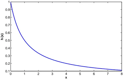
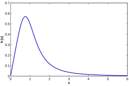
Definition 4. For a bounded function h with a negative Schwarzian derivative, we will say h is of type A if h′ is a strictly decreasing function, and of type B otherwise. The two types of functions are illustrated by the help of Figures 2.1 and 2.2. 0 1 2 3 4 5 6 7 8 0.1 0.2 0.3 0.4 0.5 0.6 0.7 0.8 0.9 1 x h ’ (x)
0 1 2 3 4 5 6 0 0.1 0.2 0.3 0.4 0.5 0.6 0.7 x h ’ (x)
Figure 2.2: A typical x vs h′(x) graph for type B function.
Also note that whether the function h is of type A or B, we always have
lim
t→∞h
′
(x) = 0. (2.51)
Remark 2.5.2. It is easy to determine whether a function h is of type A or B.
If h′(0) = 0, then it is clear that the function h is of type B. If we have
h′(0) > 0, (2.52)
and h′′(0) > 0 then h(x) is of type B. If (2.52) is satisfied and
h′′(0) ≤ 0, (2.53)
then h is of type A.
Remark 2.5.3. Suppose the function h is defined as follows:
h(x) = g◦ g(x), (2.54)
where g is a function defined fromR+ to X ⊆ R+ such that
Sg(x) < 0 and g′(x) < 0 ∀x ∈ (0, ∞). (2.55) Then, by the convolution property of the Schwarzian derivative, we have
Sh(x) < 0 ∀x ∈ (0, ∞). (2.56)
1. x0 is a fixed point of g.
2. x0 < g(x0), so h(g(x0)) = g(g(g(x0))) = g(x0) and h has another fixed
point greater than x0.
3. g(x0) < x0, so h(g(x0)) = g(g(g(x0))) = g(x0) and h has another fixed
point less than x0.
Two examples of functions satisfying the conditions in 2.5.3 are Hill functions and the tangent hyperbolic function. The gene regulatory network, which we will analyze in Chapter 3, has nonlinearities in the form of Hill functions. Hence, Assumptions in 2.5.3 does not limit us.
Proposition 1. Let f be a function of the form given in (2.54) with g satisfying the assumptions given in Remark 2.5.3 and x0 be the unique fixed point of g.
Then, we have the following:
1. If|g′(x0)| < 1, then h has the unique fixed point x0.
2. If h is of type A, then h has the unique fixed point x0 satisfying
h′(x0) < 1.
3. If h is of type B and
(i) h′(x0) < 1 then h has the unique fixed point x0.
(ii) h′(x0) > 1 then h has exactly three fixed points.
Proof. First note that since g is a strictly decreasing function, we have
g(0) > g(x) > 0 ∀x > 0, (2.57) so g is a bounded function which implies that the function h is bounded. Since g is a decreasing function, it has a unique fixed point x0. Observe that
Since
g′(x) < 0 ∀x ∈ (0, ∞), we have
h′(x) > 0 ∀x ∈ (0, ∞).
At the unique fixed point x0 of g, we have the following equality:
h′(x0) = g ′ (g(x0))g ′ (x0) = (g ′ (x0))2. Therefore, we have |g′(x0)| < 1 ⇔ h ′ (x0) < 1 |g′(x0)| > 1 ⇔ h ′ (x0) > 1.
We have shown that the function h is either of type A or type B. Therefore, if we prove second and third part of the Proposition then the first part is follows straightforwardl. For the first part of the Proposition assume that the function h is of type A, then h′ is strictly decreasing inR+. Notice that since h is bounded,
we have lim x→∞(h ′ (x)) = 0. If h′(x0)≥ 1, then since h ′
is a decreasing function we have
h′(x) > 1 ∀x ∈ [0, x0].
From mean value theorem for some t∈ [0, x0] we have the following:
h′(t) = h(x0)− h(0) x0
≤ x0− h(0)
x0
≤ 1. But on the other hand we have
h′(x) > 1, ∀x ∈ [0, x0],
so we arrived to a contradiction. Therefore, we have h′(x0) < 1. Now, suppose
there exists another fixed point of the function h. We know from Remark 2.5.3 this implies that
But mean value theorem implies that there exists t∈ [x0, y] such that
h′(t) = h(y)− h(x0) y− x0
= 1.
Since h′(x) is a strictly decreasing function, we have
h′(x) < 1 ∀x ≥ x0. (2.58)
Therefore, h has the unique fixed point x0. For the third part of the Proposition,
we assume that h is of type B. We define a new function in the following way:
f (x) = x− h(x). (2.59)
Then clearly we have
f (0) < 0 and f′(x) = 1− h′(x). (2.60) Note that the zero crossings of the function f and the fixed points of the function h are the same. Suppose that
h′(x0) < 1. (2.61)
Also assume that the function h has a fixed point y which is different from x0.
From Remark 2.5.3, we can safely assume that
y < x0. (2.62)
Again from Remark 2.5.3 we have another fixed point of h which is denoted by z and is greater than x0. For type B functions, we have either
h′(x) < h′(x0) < 1 ∀x ∈ [0, x0] (2.63)
or
h′(x) < h′(x0) < 1 ∀x ∈ [x0,∞]. (2.64)
If the condition (2.63) is satisfied then we have f (0) < 0 and
Then it is clear that f (y) < 0; so, in other words, we have
f (y) ̸= 0 (2.66)
which is a contradiction. For the case in equation (2.64) using a similar argument we can show that f (z) ̸= 0. Hence, if (2.61) is satisfied, then h has the unique fixed point x0. Now, let us assume that
h′(x0) > 1. (2.67)
But for a type B function h, we can have at most two different values such that t1 and t2 such that
h′(ti) = 1 for i = 1, 2. (2.68)
Hence f can have at most three zero crossings which implies that the function h has at most three fixed points. From (2.67) we can deduce the following
∃x1 > x0 such that f (x1) < 0, (2.69)
but since the function h is bounded we have
lim
t→∞(f (x)) =∞. (2.70)
Therefore, f has a zero crossing greater than x0, thus h has a fixed point greater
than x0. But we know that the function h has at most three fixed point. From
Remark 2.5.3 we can conclude that h has exactly three fixed points.
The results we obtained in Proposition 1 is vital for our discussion in Chapter 3. Although in Proposition 1 we assumed that the function h is in a special form given by (2.54), the following Corollary gives a more general result.
Corollary 2.5.2. Let h be a bounded function from R+ to Y ⊆ R+ with
Sh(x) < 0.
Proof. Let p(x) = x− f(x), then from the proof of Proposition 1, p can take the value 0 at most three times. Therefore, the function h can have at most three fixed points.
Remark 2.5.4. In Corollary 2.5.2, we showed that a function h having negative
Schwarzian derivative may have at most 3 fixed point. Suppose that h has exactly 3 fixed points and denote this three fixed points as y1, y2 and y3 which satisfies
y1 < y2 < y3. (2.71)
From the proof of Proposition 1, we can conclude the following inequalities:
h′(y1))≤ 1, h
′
(y2)≥ 1, h
′
(y3)≤ 1. (2.72)
In fact, the second item in Proposition 1 is valid for any function h with Sh(x) < 0. But we will return to this point in Chapter 3. We close this section with another Corollary of Proposition 1.
Corollary 2.5.3. Let h be a function of the form given in (2.54) with g satisfying the conditions given in Remark 2.5.3 and let x0 be the unique fixed point of the
function g. Then, h is either Type A or Type B. If
|g′(0)| > 1, (2.73)
then the function h has the unique fixed point x0 satisfying
h′(x0)≤ 1.
Proof. The proof is very similar to the proof of the third part of Proposition 1. If h is of type A, we are done already since it is just part two of Proposition 1. Therefore, suppose that h is of type B. Let
f (x) = x− h(x). Then, since we have
h′(x) = 1 just for one point. Therefore, f can take the value 0 only twice, but the function h has either one fixed point or three fixed points. Therefore, h has a unique fixed point. But we know that
h(x0) = g(g(x0)) = x0.
If we have
h′(x0) > 1,
then, from the proof of Proposition 1, we know that the function h has three fixed points, which is a contradiction. Therefore, we have
Chapter 3
Gene Regulatory Networks
3.1
Problem Formulation
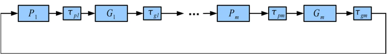
In this section we will be concerned with the asymptotic stability of a class of biological systems, the so-called gene regulatory networks which contains a feed-back loop and time delays. Basically, a gene regulatory network can be described as the interaction of DNA segments with themselves and with other biological structures such as enzymes. Gene regulatory networks can be thought as an in-dicator of the genes transcription rates into mRNA, which is used to deliver the coding information required for the protein synthesis, [24]. The proteins synthe-sized have two main duties either they can be used to give stiffness and rigidity to certain biological components such as the cell wall or they are enzymes which has the vital duty of catalyzing chemical reactions that take place in our body. Gene regulatory networks can be modeled by either a Boolean network or a set of continuous differential equations. In this work, we analyze a continuous time cyclic model given in Figure 3.1.
Figure 3.1: A continuous time model of Gene Regulatory System
Here Gi is a stable first order filter whose input is a nonlinear function of the
delayed output of Pi. Similarly Pi is a stable first order system whose input is a
nonlinear function of the delayed output of Gi−1 for 1 ≤ i < m − 1 and P1 has
an input which is a nonlinear function of the delayed output of Gm.
A continuous time model of the gene regulatory network in Figure 3.1 is proposed in [25]. The model comprises of a set of differential equations given in (1.1). Models similar to (1.1) are frequently encountered in the modeling of biological processes such as mitogen-activated protein cascades and circadian rhythm generator [12], [11], [2] and [26]. In [25], Chen and Aihara analyzed a simplified version of the system (1.1) and proved a local stability result. In the current work, we will assume that the functions fi(x) are nonlinear and have
negative Schwarzian derivatives. In this work, we will analyze system (1.4) which is obtained from (1.2) with the linear transformation given in (1.3). For the sake of clarity, we will rewrite the system model we analyze in this chapter.
˙x1(t) = −λ1x1(t) + g1(x2(t))
˙x2(t) = −λ2x2(t) + g2(x3(t))
.. .
˙xn(t) = −λnxn(t) + gn(x1(t− τ)). (3.1)
We suppose that the system (3.1) satisfies the following assumptions:
Assumption 1 For all i = 1, 2, ..., n, λi > 0.
Assumption 2 For all i = 1, 2, ..., n, the nonlinearity functions gi satisfy the
following conditions:
(ii) We have either
g′i(x) < 0 or gi′(x) > 0 ∀x ∈ (0, ∞). (3.2) Assumption 2 simply means that the functions gi are monotone and take positive
values. The nonlinearity functions have R+ as their domain since their domain
represents biological variables which take positive values. Also note that the condition g′i(0) = 0 is allowed, since it does not violate the monotonicity of the functions gi. Let us define the following function:
g = ( 1 λ1 g1)◦ ( 1 λ2 g2)◦ ... ◦ ( 1 λn gn). (3.3)
We say that the gene regulatory network is under negative feedback if
g′(x) < 0 ∀x ∈ (0, ∞). (3.4) Conversely, the gene regulatory network is said to be under positive feedback if the above inequality is reversed. It can be easily concluded that under negative feedback g defined in (3.4) has a unique fixed point. In system (3.1) the nonlin-earities are only due to the functions gi and in biological systems they often have
the Hill function form, which we discussed in Chapter 2. The system (3.1) has been analyzed by Enciso in [10]. In [10], Enciso considered the system 3.1 under negative feedback and based on the results of [9], [16], [17] and [26], he proved that if
|g′(x0)| < 1, (3.5)
then the solutions of the system (3.1) converges to the unique equilibrium point. He also proved existence of periodic solutions by a Hopf bifurcation analysis. In this work we get the same global stability result by the help of Theorem 1 of [5]. By using the results of Chapter 2, it is easy to see that the violation of (3.5) implies the local unstability of the linearized system. Combining this fact with the result of [4], we will conclude existence of periodic solutions. Moreover, we also present a result regarding the upper and lower bounds regarding possible periodic solutions. We have also proved a global stability result regarding the
homogenous gene regulatory network under negative feedback involving nonlin-earities in the form of Hill function. Furthermore, we also considered system (3.1) under positive feedback and proved some global stability results by the help of [18]. Although the nonlinearities in (3.1) are often in the form of a Hill function, the results we obtained is valid for any kind of nonlinearity functions having negative Schwarzian derivatives which includes Hill functions as a subset. For the proofs of the results we will obtain in this section, we will frequently refer to the results we obtained in Chapter 2 regarding the fixed points of functions with negative Schwarzian derivatives.
3.2
Analysis of the Gene Regulatory Network
Let our system be in the form of (3.1) satisfying Assumption 1 and 2. In the previous section we defined the following function:
g = ( 1 λ1 g1)◦ ( 1 λ2 g2)◦ ... ◦ ( 1 λn gn). (3.6)
Since the constants λi’s are positive by Assumption 1, the function g defined in
(3.6) is a well defined function onR+. As a result of Assumption 2 and the chain
rule, we have
g′(x) < 0 or g′(x) > 0 ∀x ∈ R+. (3.7)
When g′(x) < 0 we will say that the system (3.1) is under negative feedback and g′(x) > 0 is referred as the positive feedback case. We will deal with both cases separately and present some results regarding their stability and existence of periodic solutions if any.
3.2.1
Gene Regulatory Networks under Negative
Feed-back
In this section, we will consider the system (3.1) under negative feedback. That is g defined in (3.6) satisfies:
g′(x) < 0 ∀x ∈ (0, ∞). (3.8) We start this section with a Lemma regarding the equilibrium points of the system (3.1) under negative feedback.
Lemma 13. Consider the system in the form (3.1) satisfying Assumptions 1 and
2 under negative feedback. Then, the system has a unique equilibrium point in Rn
+.
Proof. The function g defined in (3.6) is decreasing and we have
g(0)≥ 0.
Therefore, by Lemma 6, we conclude that the function g has a unique equilibrium point. Let x ∈ Rn
+ be an equilibrium point of the system. We have
x1 = 1 λ1 g1(x2) .. . xn = 1 λn gn(x1)
which is in the form of Lemma 8. Therefore, the system (3.1) under negative feedback has a unique equilibrium point in Rn+.
Lemma 14. For the system (3.1), Rn
+ is a positively invariant set and for any
set of initial conditions the corresponding solution of the system remain bounded.
Proof. To prove positive invariance, we need only check the direction of the vectors on the boundaries of the region
Rn ={(x