SPECTROGRAM IMAGES BASED IDENTIFICATION OF BIRD SPECIES USING CONVOLUTIONAL NEURAL NETWORKS

SPECTROGRAM IMAGES BASED

IDENTIFICATION OF BIRD SPECIES USING

CONVOLUTIONAL NEURAL NETWORKS

2021

MASTER THESIS

COMPUTER ENGINEERING

Jutyar Fatih AWRAHMAN

Thesis Advisor

SPECTROGRAM IMAGES BASED IDENTIFICATION OF BIRD SPECIES USING CONVOLUTIONAL NEURAL NETWORKS

Jutyar Fatih AWRAHMAN

T.C.

Karabuk University Institute of Graduate Programs Department of Computer Engineering

Prepared as Master Thesis

Thesis Advisor

Assoc. Prof. Dr. Hakan KUTUCU

KARABUK January 2021

I certify that in my opinion the thesis submitted by Jutyar Fatih AWRAHMAN titled “SPECTROGRAM IMAGES BASED IDENTIFICATION OF BIRD SPECIES USING CONVOLUTIONAL NEURAL NETWORKS” is fully adequate in scope and in quality as a thesis for the degree of Master of Science.

APPROVAL

Assoc. Prof. Dr. Hakan KUTUCU ... Thesis Advisor, Department of Computer Engineering

This thesis is accepted by the examining committee with a unanimous vote in the Department of Computer Engineering as a Master of Science thesis. Jan 27,2021

Examining Committee Members (Institutions) Signature

Chairman : Assoc. Prof. Dr.Hakan KUTUCU (KBU) ...

Member : Asst. Prof. Dr. Ümit ATİLA (KBU) ...

Member : Asst. Prof. Dr. Levent EMMUNGIL (OTU) ...

The degree of Master of Science by the thesis submitted is approved by the Administrative Board of the Institute of Graduate Programs, Karabuk University.

Prof. Dr. Hasan SOLMAZ ...

“I declare that all the information within this thesis has been gathered and presented in accordance with academic regulations and ethical principles and I have according to the requirements of these regulations and principles cited all those which do not originate in this work as well.”

ABSTRACT

M. Sc. Thesis

SPECTROGRAM IMAGES BASED IDENTIFICATION OF BIRD SPECIES USING CONVOLUTIONAL NEURAL NETWORKS

Jutyar Fatih AWRAHMAN

Karabuk University Institute of Graduate Programs The Department of Computer Engineering

Thesis Advisor:

Assoc. Prof. Dr. Hakan KUTUCU January 2021, 48 pages

The identification of bird species by their sounds is one field of research. This paper focuses on identifying bird species based on spectrogram images using Convolutional Neural Networks (CNN). This is more than a challenge when talking about advanced identification of bird species using spectrogram analysis. Different CNN architecture models and representations of the spectrum have been trained, validated, and tested on 10600 audio instances, which belongs to 437 various classes in our dataset. We had concluded that CNN allows achieving good results since it eliminates the potential modeling errors from results of the incomplete or inaccurate bird species knowledge. The models were implemented by using the Python programming language and the Librosa library. The bird sounds have been obtained from different areas in Turkey, and we performed pre-processing operations to create a spectrogram dataset. We divided the label sounds for training, testing, and validation. Then, the samples were

put into 10-folds. The system trains for 150-epochs and the loss is 0.7759 and the overall training accuracy stands at 0.94.

Keywords : Birds sound dataset, Classification, CNN, Spectrogram. Science Code : 92431

ÖZET

Yüksek Lisans Tezi

KUŞ TÜRLERİNİN KONVOLÜKSİYONEL SİNİR AĞLARI KULLANILARAK SPEKTROGRAM GÖRÜNTÜLERİ TABANLI

TANIMLANMASI

Jutyar Fatih AWRAHMAN

Karabük University Lisansüstü Eğitim Enstitüsü Bilgisayar Mühendisliği Anabilim Dalı

Tez Danışmanı: Doç. Dr. Hakan KUTUCU

Ocak 2021, 48 sayfa

Kuş türlerinin sesleriyle tanımlanması bir araştırma alanıdır. Bu makale, Evrişimli Sinir Ağlarını (CNN) kullanarak spektrogram görüntülerine dayalı olarak kuş türlerini tanımlamaya odaklanmaktadır. Bu, kuş türlerinin spektrogram analizi ile ileri düzeyde tanımlanmasından bahsederken bir zorluktan fazlasını temsil eder. Spektrumun farklı CNN mimari modelleri ve temsilleri, veri setimizdeki 437 farklı sınıfa ait 10600 ses örneği üzerinde eğitilmiş, doğrulanmış ve test edilmiştir. CNN'in, eksik veya yanlış kuş türleri bilgisinin sonuçlarından kaynaklanan potansiyel modelleme hatalarını ortadan kaldırdığı için iyi sonuçlara ulaşılmasına izin verdiği sonucuna vardık. Modeller Python programlama dili ve Librosa kütüphanesi kullanılarak gerçekleştirildi. Kuş sesleri Türkiye'nin farklı bölgelerinden elde edildi ve bir spektrogram veri seti oluşturmak için ön işleme işlemleri gerçekleştirdik. Etiket seslerini eğitim, test ve doğrulama için böldük. Daha

sonra numuneler 10 katına konuldu. Sistem 150 dönem için eğitim alır ve kayıp 0,775922'dir ve genel eğitim doğruluğu 0,94'tür.

Anahtar Kelimeler : Kuşlar ses veri seti, Sınıflandırma, CNN, Spektrogram. Bilim Kodu : 92431

ACKNOWLEDGMENT

Firstly, I thank God deeply in my heart, and my advisor, Assoc. Prof. Dr. Hakan KUTUCU, for his limitless interest contribution and interest in the preparation of this thesis. Also, I would also like to show my gratitude to my family, who stood by my side throughout my journey, especially my parents for their limitless contribution. I would also want to thank my wife for her amazing support and courage. I am more than grateful for the assistance and contribution from my friend Ghazi and my cousin Drust through the obstacles. Also, I thank all my friends who were with me during my study.

CONTENTS Page APPROVAL ... ii ABSTRACT ... iv ÖZET ... vi ACKNOWLEDGMENT ... viii CONTENTS ... ix

LIST OF FIGURES ... xii

LIST OF TABLES ... xiii

ABBREVIATIONS ... xiv PART 1 ...1 INTRODUCTION ...1 1.1. MOTIVATION ... 2 1.2. PROBLEM STATEMENT ... 2 1.3. FEATURE EXTRACTION... 3

1.4. AIMS OF THE STUDY ... 3

1.5. THESIS STRUCTURE ... 4

PART 2 ...6

RELATED WORK ...6

2.1. SPECTROGRAM ... 8

2.2. MACHINE LEARNING APPROACHES ... 9

2.3. DEEP LEARNING APPROACHES ... 10

2.4. CONVOLUTIONAL NEURAL NETWORKS (CNN) ... 11

2.4.1. Convolution Layer: ... 11

2.4.2. Pooling Layer ... 12

2.4.3. Fully Connected Layers (FC) ... 13

Page

2.4.6. Loss Function ... 15

2.4.7. Dropout Learning ... 15

2.4.8. Regularization ... 16

2.4.9. Early Stopping ... 16

2.4.10. K-Fold Cross Validation ... 16

2.4.11. Batch Size ... 16

2.5. MEASUREMENT AND EVALUATION ... 16

PART 3 ...19

METHODOLOGY ...19

3.1. DATASET DETAILS ... 19

3.2. SPECTROGRAM CALCULATION ... 19

3.2.1. Chroma-STFT (Short-Time Fourier Transform) ... 20

3.2.2. Mel Frequency Cepstral Coefficients (MFCCs) ... 20

3.2.3. Mel-Spectrogram ... 21

3.3. PREPROCESSING AND SEGMENTATION ... 21

3.4. SYSTEM MODELING ... 23 3.4.1. Convolution Layer ... 23 3.4.2. Pooling Layer ... 24 3.5. IMPLEMENTATION ... 26 3.5.1. Representation of Audios ... 26 3.5.2. CNN Models ... 31 PART 4 ...36 RESULTS ...36 PART 5 ...38 5.1. DISCUSSION ... 38 5.2. ANALYSIS OF STUDY ... 39 PART 6 ...41 6.1. CONCLUSION ... 41 6.2. FUTURE WORK ... 41

Page REFERENCES ...42

LIST OF FIGURES

Page

Figure 2.1. Representation of spectrogram ... 8

Figure 2.2. Comparison between machine learning and deep learning ... 10

Figure 2.3. Representation of Convolutional Neural Network ..…………...……….11

Figure 2.4. Operation of the convolution network ………...………..……12

Figure 2.5. The representation of the max pooling process . ... 13

Figure 2.6. The operation of the Fully Connected layer ... 13

Figure 2.7. The dropout Strategy (a) without dropout (b) with dropout...………...15

Figure 2.8. Representation of AUC - ROC ………...……….18

Figure 3.1. Representation of Chroma-STFT with 12 dimensions ... 20

Figure 3.2. Representation of MFCC with 20 dimensions ... 21

Figure 3.3. Mel spectrogram with 128 dimensions ... 21

Figure 3.4. Segmentation of bird sounds ... 22

Figure 3.5. Flowchart of the training of identification models. ... 23

Figure 3.6. Parameters of CNN models used in the study (a)first model (b) second model……….………..……...25

Figure 3.7. Plot of training and validation accuracy and lossusing Chroma-STFT ... 27

Figure 3.8. Plot of training and validation accuracy and loss using MFCC ... 28

Figure 3.9. Plot of training and validation accuracy and loss using Mel spectrogram ... 29

Figure 3.10. Plot of training and validation accuracy and loss using mix sound transform to the spectrogram ... 30

Figure 3.11. Plot of training and validation accuracy and loss using the first model ... 32

Figure 3.12. Plot of training and validation accuracy and loss using the second method ... 33

Figure 3.13. Plot of training and validation accuracy and loss using the third method ... 34

LIST OF TABLES

Page

Table 1. Representation of Confusion Matrix with 2 species. ... 17

Table 2. Feasible hyper parameters when using the first model. ... 31

Table 3. Feasible hyper parameters when using the second model. ... 33

Table 4. Summary of above results with accuracy and loss. ... 36

Table 5. Summary of our CNN model’s results. ... 37

Table 6. Comparison of the results of our CNN model on Urban Sound and thesis dataset... 37

ABBREVIATIONS

ANN : Artificial Neural Network

CNN : Convolutional Neural Network

RNN : Recurrent Neural Network

RELU : Rectified Linear Units

Tanh : Hyperbolic Tangent

SVM : Support Vector Machines

LSTM : Long Short-Term Memory

FC : Fully Connected Layer

ML : Machine Learning

C-MAP : Classification Mean Average Precision

MFCC : Mel Frequency Cepstral Coefficients

1 PART

INTRODUCTION

An important issue in ecology is interaction between organisms and their environments, monitoring the populations of animals, due to the threat of climate change [1].

The use of acoustics to classify and monitor animals in their environments has lately become a subject of interest [2, 3]. Using recorded sound data for animal species classification is useful for monitoring biodiversity, breeding, and population dynamics [4, 5]. Birds can be particularly helpful for ecological indicators, because they react quickly to environmental changes. Domain experts can be used for bird classification; however, as data increases, this becomes a long and tedious process. Therefore, tools are needed to improve the process.

The aim of this research is to detect and classify bird species using a Convolutional Neural Network (CNN). The detection of bird species is a useful issue to solve, and it has been a major cause of birds’ conservation for many years. One of the most common problems of bird species detection is the fact that bird species fall into several types [6]. Speech researchers are worked on imagine data in the early stages in 1960s and the spectrogram was used, Representation of information by using spectrogram produced a good feature for sound classification [7].

features can be obtaining from audio signals [8]. Audio systems are highly advanced nowadays, yet there are still a lot of false results, especially due to non-bird’s structures [9]. Due to the differences between negative and positive proportions, the system always tries to classify the regions and use some of them later. To increase the accuracy of a detection system, separate models are used for classification [10].

Many techniques have been used for the classification process, and some of them feature extraction using classical computer vision with machine learning [11, 12].

With the improvement of the deep neural network, many new architectural models appear. Hence, it is critical to assess which provide the finest execution, with the lowest time utilization. In some cases, exceptionally deep neural network systems are overkill for a specific task, whereas using less complex strategies can produce comparable results while, at the same time, sparing assets. Subsequently, working on each issue needs detailed and a lot of studies.

1.1 MOTIVATION

Identifying bird species by their sound is a difficult task if done manually, since there are hundreds of types of bird species in the wild. Automated processing using artificial intelligence specially using deep neural network can identify bird species with good results. In this research, we would like to work on identifying bird species according to their sound in Turkey, so my dataset consists of bird sounds obtained from different areas in Turkey. Since Convolutional Neural Networks have had huge successes in most classification tasks, this study also adopts them, along with the use of spectrograms to represent or extract sound features.

1.2 PROBLEM STATEMENT

With bird species detection, some problems will appear, such as the bird species fall into several types, collecting a high amount of data with a large number of species when some records contain more than one species. The research is trying to answer the following questions that cover Data acquisition and the Convolutional Neural Network.

 Is using spectrogram analysis measurements for audio samples via a CNN an

appropriate method for bird species detection?

 Does using audio features as an image spectrogram impact the performance of

 Which library should be used with Python for better performance?

 What should be the pipeline of implementation for converting audio to spectrograms?

1.3 FEATURE EXTRACTION

Another issue when training neural networks is deciding what features to use as input into the network. Furthermore, it is necessary to determine how to extract features that contain as much information about the original input as possible, but with a lower dimensionality, to enable efficient training [13]. The design of a feature extraction method can be seen as a trade-off between separability and compactness [14].

1.4 AIMS OF THE STUDY

This research includes the following achievements:

 Providing a summary of previous works.

 Identifying bird species using their sounds with high accuracy and good performance.

 Using bird sounds obtained from different areas in Turkey as data.

 Showing that a Convolutional Neural Network (CNN) can be used to classify

sounds, as well as images.

 Proving spectrograms offer a high capacity for using CNN models to classify audio.

 Evaluating and comparing the used CNN models on these sounds among themselves and with others.

1.5 THESIS STRUCTURE Part 1. Introduction of the thesis

This Part contains the background, motivation, and problem statement. It also describes the aims of this study.

Part 2. Background

We highlight some previous work and research conducted in the field of our problem. We offer some introductory background needed for this thesis. In particular, we illustrate the definitions of a spectrogram and Convolutional Neural Network and the functioning of the latter. This part shows the steps for detecting bird species using a CNN.

Part 3. Methodology

This part describes the approaches used for bird classification. Here, we specify in detail the full processes of representing spectrograms and implementing CNNs. During the implementation, we also perform experiments.

Part 4. Results

We conduct a careful evaluation of our representation of the spectrum and methods in the Convolutional Neural Network. Those results are reported and compared to those of other methods used for other classifications.

Part 5. Discussion

We compare existing studies with the results of this research. We highlight differences between these prior studies and what is achieved here by providing an analysis of the study.

Part 6. Conclusions

We provide a summary and conclusion of the results obtained in this thesis, as well as its contributions. The same part offers a short description of potential future work.

2 PART

RELATED WORK

This thesis works to identify bird species according their sounds using a Convolutional Neural Network (CNN). Recently, CNNs have achieved high performance in many areas of natural language processing. In this section, we present the latest research and projects related to our work.

Jaiswal et al. [15] used a Convolutional Neural Network as a method to classify sounds. The dataset used consisted of various urban sounds and spectrograms generated from these sounds, to be used by a CNN, and various layers were used. Although the accuracy of state-of-the-art methods was 78%, the accuracy achieved by this paper was 85%.

Xie et al. [16]worked on acoustic and visual features and used a CNN for bird sound classification. Their dataset consisted of 14 bird species, and the best achievement of their study was an F1-score of 95.95% through the fusion of acoustic features, visual features, and deep learning.

Zottessoet al. [17] used textural features derived from spectrogram images and a dissimilarity framework they started by recording audio of eight challenging subsets from LifeClef 2015, the range of classes numbering from 23 to 915. They achieved an identification rate of 71%, considering 915 species in the hardest scenario.

Ozer et al. [18] worked on recognizing sounds automatically using computers, as some previous methods displayed weak performance when including noise. After some conversions, first from overlapped spectrogram to linear image with reduced dimensions, then feature extraction, then finally classification with a CNN using their method, their work achieved a performance improvement of 4.5% and classification success of 97.4%.

Machine Learning for Signal Processing-2013. [19]: In this competition, 79 teams participated in a challenge to identify bird species given data sets of bird sounds taken from the real world. The dataset consisted of 645, each record being ten seconds long and the dataset as a whole covering a total of 19 bird species. Datasets were split into 50% training and 50% testing. The results of this competition showed that automatic sound recognition (ASR), which uses machine learning (ML) in a real environment, is appropriate for collected audio with multiple vocalizing birds at the same time, as well as noises like car sounds, rain, etc. As a result, Convolutional Neural Networks achieved a good result.

Bai et al. [20] worked on a system for identifying birds based on an inception model with some techniques of data augmentation, working on BirdCLEF, and extracting features using a log-mel spectrogram. They chose an inception-v3 model, which allows more extracted features and has fewer parameters. They added data augmentation to prevent overfitting and improve performance, and the model achieved 0.055 of classification mean average precision (c-mAP).

Küc̣üktopcu et al. [21] worked on a model to recognize the sounds of birds. The model is a composite of three basic hardware elements, namely a microphone, a microcontroller, and a storage unit. First, they recorded sounds from the environment. Then, they removed noise. The final proposed system conducts feature extraction and the classification of bird species. They store the processed data on an SD card.

This research presents some methods for changing sound to an image (spectrogram), feature extraction from bird sounds, and the classification of birds using a CNN.

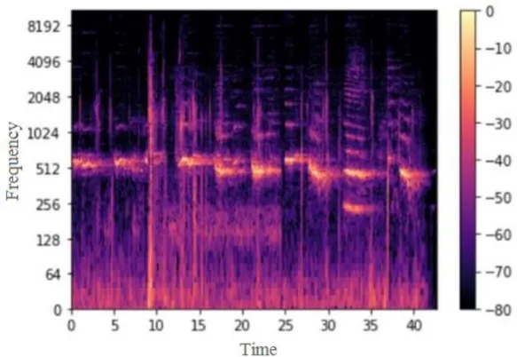
Figure 2.1. Representation of spectrogram 2.1 SPECTROGRAM

A spectrogram is the representation of a signal with different frequencies over different times. Both the vertical and horizontal axes of a spectrogram represent the frequency and the time of the signals that have been converted into the spectrogram. It contains more information than other types of time-frequency. A spectrogram can be used to show bird sounds by converting the vocals to various signals and those signals to a spectrogram. After that, the spectrogram can be used to differentiate each bird species from the others [22]. An example Spectrogram is shown in Figure 2.1.

2.2 MACHINE LEARNING APPROACHES

Artificial intelligence and machine learning have been used for tasks like image classification and natural language processing [24]. machine learning has always been used for classifying bird species, and such methods always follow the same pattern [25]:

 Image Preprocessing: This involves calculating the positions and important points of a photography; preprocessing images usually gives them more features.

 Segmentation: this process extracts the main part of the image, and it can remove the background of the image.

 Feature extraction: features are extracted from the image to distinguish its important parts. This can reduce the complexity of the process, and allow most of the work to be done in a shorter time.

 Classification: Extracted features can be extended by some ML algorithms,

including SVMs, K-nearest Neighbor classifications, and decision trees.

Differences between traditional machine learning and deep learning have surfaced in feature engineering: traditional machine learning uses handcrafted feature extraction, while deep learning uses automatic feature extraction. Manual feature extraction is difficult and also requires more time, while automatic feature extraction is more accurate. The differences between machine learning and deep learning are shown in Figure 2.2.

Figure 2.2. Comparison between machine learning and deep learning [26].

2.3 DEEP LEARNING APPROACHES

Deep learning is an important trend in machine learning, it has a high accurate with a high performance to detect of objects, deep learning needs a huge number of data, it has always been difficult to obtain huge information from an open source, also it can be used on an unsupervised data. using deep learning needs more time for training, so by using GPU training time can be reduce [27].

In this research, we focus on using supervised learning and a deep neural network (Convolutional Neural Network) to classify the dataset, so two main research trends can be visualized: first, a strategy using good CNN architectures, then another approach that aims to use the large datasets applied to the classification.

2.4 CONVOLUTIONAL NEURAL NETWORKS (CNN)

A CNN is a class of neural network, currently CNN gained a popularity at image detection. The classification of handwriting was carried out by LeNet, AlexNet which made a set of performance metrics for the CIFAR dataset [28].

CNN has become more popular due to its massive success in a lot of tasks across classification, image segmentation, and object tracking. CNN derives its extensions and processing methods from brain structures [29]. It consists of several layers: first an input layer, then several convolutional layers and a pooling layer, then one or more fully connected layers, and finally the output layer [30], as shown in Figure 2.3.

Figure 2.3. Representation of Convolutional Neural Network.

2.4.1 Convolution Layer

The primary part of a CNN is convolution activity. it is a cross-connection. In PC vision applications, convolution is constantly done between the bit (channel) and the picture. The fundamental motivation behind these activities is to extract the features. The required preprocessing in a CNN is much less than for other conventional

that were hand-designed using traditional techniques [31]. The learnable weights and bias in CNN are more impressive than human exertion and information, the operation of the convolution network is shown in Figure 2.4.

Figure 2.4. Operation of the convolution network [32].

The two layers that come after the convolution layer, namely the pooling layer and fully connected layer, are two important layers of CNN.

2.4.2 Pooling Layer

This is one of the CNNs’ layers, the extracted feature sets are then passed to the pooling layer. Pooling may compute the maximum or average, depending on the application; in this layer, images are shrunk down while preserving the most important information in them. The dimensions of the data is reduce by the pooling layer, and the max pooling

layer also preserves the maximum value from each window [33, 34], as shown in Figure 2.5.

Figure 2.5. The representation of the max pooling process [35].

2.4.3 Fully Connected Layers (FC)

The last layer is the fully connected layer. This connects every neuron in the previous layer to every neuron in the next layer. The FC layer is one of the features of a CNN that classifies the features previously received from other layers [36]. The fully connected layer with input and output layers is shown in Figure 2.6.

2.4.4 Hyperparameters

Hyperparameter consists of the variables that is used to specify the structure of the network. It makes an optimal performance for the model. By using adjustable parameters, it makes the model deploy and faster.

2.4.5 Activation Functions

These make deep neural network learning easier by offering non-linearity. Also, they give the learning process the ability to handle complex tasks [38].

The system has been tested with different activations, such as Hyperbolic Tangent

(Tanh), Softsign, Exponential Linear Unit (ELU), soft Plus, sigmoid, and ReLU. In

the end, we used SoftMax as the classifier [39].

2.4.4.1 Hyperbolic Tangent

This formula has been used as a normal non-linear function in setting up multiple layers of the perceptron. The range is from (-1 to 1)

𝑓(𝑥) = 2

1+ 𝑒−2𝑥− 1 (2.1)

2.4.4.2 Rectified Linear Units

Now the deep architectures are replaced with new solutions. One of these is the ReLUs

𝑓(𝑥) = {0 𝑓𝑜𝑟 𝑥 < 0

𝑥 𝑓𝑜𝑟 𝑥 ≥ 0 (2.2)

A ReLU is a different unit from the traditional ones, and it has more benefits. Its speed is higher while computing, and it is more powerful when propagating gradients (sigmoid units have saturation, but ReLUs do not), the range of RELU is (0 to infinity), retaining different properties while simplifying the structures.

Different units might end up in the dead zone depending on their random weight initialization, and given zero gradients. Therefore, this project uses Tanh, ReLU as activation function and softmax for classification.

2.4.6 Loss Function

The loss function is a technique to measure the performance of the network model on the labeled data. Cross-entropy and mean squared error(MSE) are both common loss functions. They can compute what differently, which can help the optimization of the gradient [13].

2.4.7 Dropout Learning

Some approaches to deep neutral network architecture there is a tendency toward overfitting. This can bring about a bad shortage of samples. Dropout learning is a way to solve this issue. The dropout is a technique has been used to prevent or reduce overfitting and improving the performances [40, 41].

The idea is very straightforward, yet profoundly successful: in each training cycle, a concealed unit is arbitrarily eliminated with a predefined likelihood (50%), and the learning technique proceeds normally. Usually The dropout is used after the pooling layer, it also can be used after convolution layer. We used a dropout of 0.4 unit. The dropout strategy is showed in Figure 2.7.

2.4.8 Regularization

This is a way of reducing model difficulty and it can be used to reduce overfitting, and adds a penalty to the loss function. L1 and L2 are the most common regularizations. L2 is better for complex models as it learns difficult patterns; however, L1 has better performance for simple models.

2.4.9 Early Stopping

This a technique is one of the regularization form, it can be used to monitor the loss to prevent overfitting on validation set, by using early stopping the process will be interrupted when the loss will increase inside the model [43].

2.4.10 K-Fold Cross Validation

K-fold cross validation is a process to evaluate or optimize the performance of classification methods on a dataset. it is used to split all samples randomly to a k-folds with an appropriate size, which the validation process is inside one fold and the remain folds for training model. The model wants to achieve an optimal result, After this process, the average accuracy of all folds must be found [44].

2.4.11 Batch Size

Batch size is a number of training instances used before updating the model. The higher batch sizes are more efficient the process. Fewer batches tend to work better with a small number of epochs. However, larger batches have more generalizations. The batch size has been set to 128 in this process.

2.5 Measurement and Evaluation

One of the major parts in any experiment is Evaluation, it is a process of explaining corrected classification of objects(dataset) by the classifier, or to explain the accuracy of classification, there are some techniques like (Confusion matrix, Accuracy, precision, recall, f1-score, ...etc.).

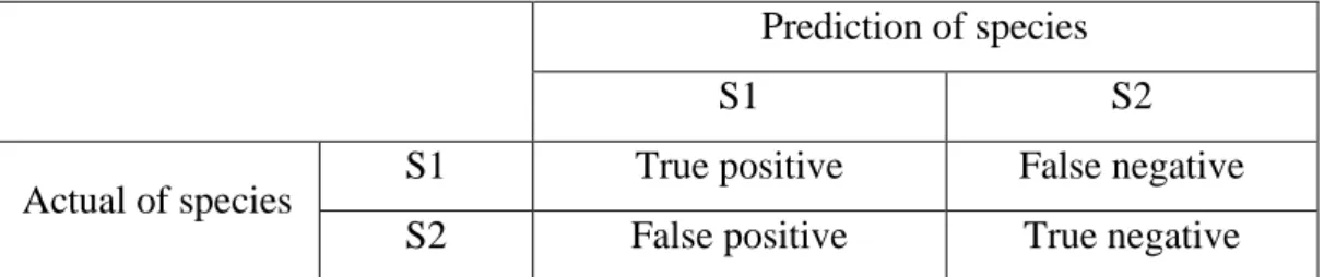
Confusion matrix is a private table that is used to show and enhance the accuracy of classification models. Inside the tables each column is used to show samples in predictive species, each row is used to show samples in actual species, and all true representations are indicated by a diagonal inside the table [45]. As shown in Table1.

Table 1. Representation of Confusion Matrix with 2 species. Prediction of species

S1 S2

Actual of species S1 True positive False negative

S2 False positive True negative

S is used to explain a species, TP consists of the True Positive numbers. FP consists of False Positive and FN is a Number of False Negative.

Accuracy is a process of explaining the ratio of correct classification samples by classifier

𝐴𝑐𝑐𝑢𝑟𝑎𝑐𝑦 = 𝑇𝑃+𝑇𝑁

𝑇𝑃+𝑇𝑁+𝐹𝑃+𝐹𝑁 (2.3)

The F1-score is usually used to show the performance of model’s accuracy in classifications by using a specific algorithm, and it is used to evaluate the accuracy of tests [46]. The F1-score is calculated from the Precision and Recall like this

𝐹1 = 2( 𝑝𝑟𝑒𝑐𝑖𝑠𝑖𝑜𝑛 𝑥 𝑟𝑒𝑐𝑎𝑙𝑙

𝑝𝑟𝑒𝑐𝑖𝑠𝑖𝑜𝑛+ 𝑟𝑒𝑐𝑎𝑙𝑙 ) (2.4)

where

Precision = 𝑇𝑃

Recall is a true positive prediction in classification process. Precision is a ratio of positive predictions were they are really true. The value of F1-score is between 0 and 1, if the value of one of them whether precision or recall equal to 0 then f1 score will be 0, if the values of both precision and recall equal to 1 then the f1 score will equal to 1 [47].

Area under curve(AUC) and Receiver Operating Characteristics (ROC) curve are one of the major evaluation metrics to evaluate classification, ROC is used as probability and AUC shows the measure of differences, it is used to show that the ability of the model is to differentiate classes, and their results are between (0 and 1), if the result of AUC near to 0 the model is going to be poor for classification, if the result of AUC near to 1, the model becomes a good measure to separate classes [48]. As shown the representation of AUC-ROC in Figure 2.8.

3 PART

METHODOLOGY

The methodology has been divided into different steps. Various representations of signals and different CNN architecture models have been used. Practically, this research has been implemented using the Python programming language and the Librosa library [49].

3.1 DATASET DETAILS

Bird sounds have been obtained from different areas in Turkey. The dataset consists of 802 bird sounds, which are in mp3 files. The files contain events from different life stages of the birds, and have different durations. All file names are in Turkish, and they have stereo channels. First, we listened to all files and found that some parts of the files contained background noises, such as humans, other animal sounds, or rain. Sound durations ranged from 3 seconds to 5.3 minutes, so we extracted the good parts of the bird sounds. Finally, we obtained 10600 .wav files with a 44.1 KHz mono channel, each 5 seconds long. The samples were put into 10-folds with 437 bird species (classes). The dataset was labeled by creating a CSV file, and all the file names, numbers of folds, and Latin names of species (Scientific names) were put in the CSV file.

3.2 SPECTROGRAM CALCULATION

A Convolutional Neural Network (CNN) works on images; therefore, the audio files first must be converted to an image format so that they can be used by the CNN [13]. Acoustics can be changed to different characteristics, and these characteristics can be used to form vectors. Extracting useful features is important for any automatic system.

Before processing, the acoustics are converted to spectrograms. These are a visualization of the frequencies of a sound considering time [22].

In this study, we used four time-frequency transform methods (Chroma-STFT, Mel-frequency cepstral coefficients (MFCCs), Mel-spectrogram, and concatenate features) to convert the sounds to spectrograms. the three figures that serve to show the time-frequency transforms (Figures 3.2.1, 3.2.2 and 3.2.3) demonstrate them using sounds from Dendrocopos leucotos which is a white-backed woodpecker as an example.

3.2.1 Chroma-STFT (Short-Time Fourier Transform)

We use the waveform to compute a Chroma-STFT. which can be used on audio samples, and the results can be displayed as a spectrum in a Chroma-gram: the notes of the audio are shown on the vertical axis in the Chroma-gram. Chroma preferences are good for representing music audio since the spectrums are shown in 12 bins that indicate distinct semitones [40], as shown in the representation of Chroma-STFT in Figure 3.1.

Figure 3.1. Representation of Chroma-STFT with 12 dimensions.

3.2.2 Mel Frequency Cepstral Coefficients (MFCCs)

Mel Frequency Cepstral Coefficients(MFCCs) can be used as a Mel-frequency spectrogram. This technique is often used in audio-related applications. A signal is a small indication, usually between 10 to 20 bins, and shows the overall view of the spectral envelope [50], as shown in the representation of MFCC with a 20-dimensional vector in Figure 3.2.

Figure 3.2. Representation of MFCC with 20 dimensions.

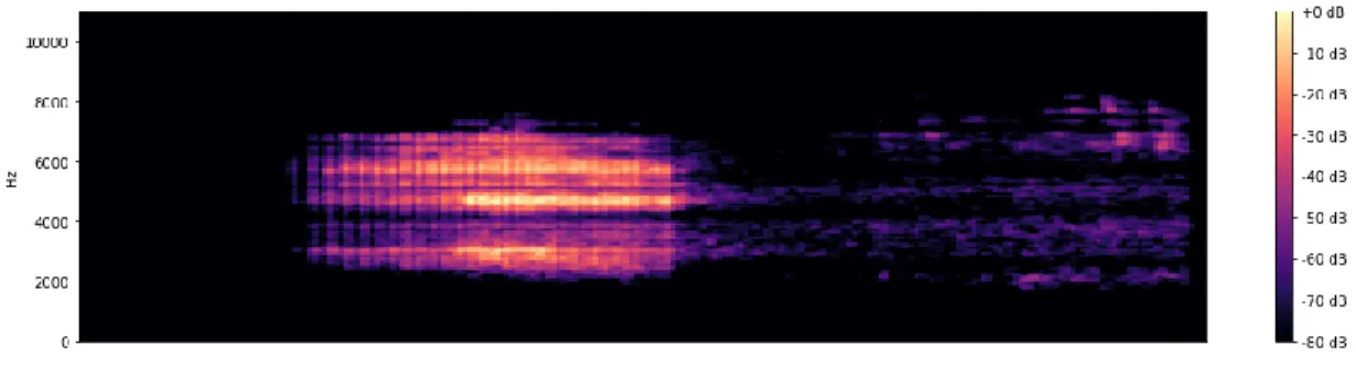
3.2.3 Mel-Spectrogram

A Mel scaled spectrogram is computed by Mel-spectrogram. This is used to represent a signal at different frequencies and different times, and the signals are usually divided into 128 bins [40]. A representation of a Mel spectrogram with 128 dimensions is shown in Figure 3.3.

Figure 3.3. Representation of Mel spectrogram with 128 dimensions.

3.3 Preprocessing and Segmentation

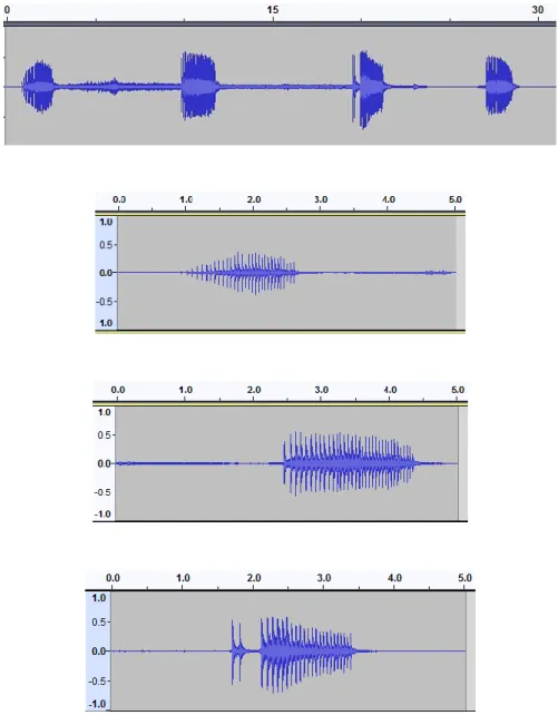
The audio files are first preprocessed into a format that can be used to train the Convolutional Neural Network and to extract major features [51]. First, we changed the audio files from stereo to mono channels and normalized them to -3 dB with a 44,100 Hz sample rate. All sounds have different durations, ranging from 3 seconds to 5.3 minutes. We split all sounds manually into 5-second segments, as shown in Figure 3.4.

Figure 3.4. Segmentation of bird sounds.

All the sample sets are randomly divided into a training set, validation set, and testing set. The ratio of this division is 8:1:1. Using these samples, the model is well trained and validated. The flowchart of the training of an identification model is illustrated in Figure 3.5.

Figure 3.5. Flowchart of the training of identification models [22].

3.4 SYSTEM MODELING

This study uses a Convolution Neural Network, because CNNs have had considerable success in most classification tasks. The CNN is inspired by the connectivity patterns of neurons. It consists of several layers: first the input layer, then several convolutional layers and a pooling layer, then one or more fully connected layers, and finally the output layer.

3.4.1 Convolution Layer:

The main portion of a CNN is the convolution operation. This is the core building block of a CNN. The main purpose of these operations is to extract features. The layer's parameters consist of a set of learnable filters (or kernels); we used 2D convolution layers consisting of different sizes of filters, and the first layer in the CNN performed convolution with a spectrogram of 160 features.

3.4.2 Pooling Layer

After the convolutional layer, the pooling layer is applied. This is used to decrease the number of parameters; images are shrunk down while preserving the most important information in them. We used a max pooling (2,2) filter with a stride of 2.

The fully connected layers come after the convolution and pooling layers. We have two fully connected layers (1024, 437) respectively.

After training methods to change sounds into a spectrogram, we need to create CNN architectures consisting of different filters and layers so as to have better results for our system and to increase the accuracy, lower the loss, and reduce overfitting for the process. The parameters of the CNN models used in the study are given in Figure 3.6.

An attempt has been made to optimize our training processing time and maintain good overall performance. We evaluated different kinds of parameter settings and found the following to be very effective.

Optimizer: these are algorithms or strategies responsible for reducing losses and providing the most accurate possible results. In this work, the Adaptive moment estimation (Adam) optimizer algorithm which is responsible for reducing the losses and for providing the most accurate possible results which has been used. It has got popular and accepted to neural network, because it is faster, improving accuracy and helps deep neural network to be successful and effectively trained.

Loss Function: it was used to make our prediction to able to predict expected outcomes. It used to update the weights by calculate the gradients. We used categorical crossentropy as a loss function because the decision boundary in this type of classification is large, and it is the best one to work with multi-class classification.

Figure 3.6. Parameters of CNN models used in the study (a)first model (b) second model.

Dropout: used to prevent or reduce overfitting, we use a dropout with (0.4) unit.

Regularization: this is a technique used to decrease complexity and overfitting in the model. L2 (0.0005) regularization was used because it is better than L1 for complex data tasks.

The padding operation is the process of adding a pixel to an image. The stride process is used to control filter convolution [52].

(a) First model.

3.5 IMPLEMENTATION

This approach uses preprocessing to arrange the spectrogram into a few stages of representation. It takes distinctive sound-based samples, with anticipated probabilities for each samples, and runs an investigation to report the general effectiveness of the framework. The models were implemented by using the Python programming language and the Librosa library. This cycle of the usage pipeline ends with a characterization of creature species, as shown in the outcome area.

Our dataset includes 10600 .wav files. The step of preprocessing and reducing noise is applied. After that, the audio files are changed to spectrograms, then the dataset is randomly separated for training, validation, and testing with a ratio of 8:1:1.

Using CNN models, we attempt to recognize bird species. For each CNN model, some of the filters and a different number of layers are changed. We train each CNN model for 100 epochs, with changing some settings to find and select the best performance according to the validation accuracy, with the best accuracy, precision, recall, and F1-score.

3.5.1 Representation of Audios

Chroma-STFT, Mel-frequency cepstral coefficients (MFCCs), Mel-Spectrogram and concatenated of all them have been used to change sounds to spectrograms and find which shows the best outcome over 100 epochs.

3.5.1.1 Chroma-STFT

Chroma-STFT is the first method we use to transform bird sounds to spectrograms, with 12 dimensions. The results show 40.7% accuracy with a loss of 3.1288. Training and validation Accuracy and Loss when using Chroma-STFT are shown in Figure 3.7.

3.5.1.2 Mel-Frequency Cepstral Coefficients

By using Mel-frequency cepstral coefficients (MFCCs) on our dataset to create a spectrogram with 20 dimensions, we achieve an accuracy of 85.7% and a loss of 0.7794. Training and validation Accuracy and Loss when using MFCC are shown in Figure 3.8.

3.5.1.3 Mel Spectrogram

Thirdly, we used a Mel spectrogram to form an image from sound, with 128 dimensions. This type of spectrogram has a total number of parameters of 1336499, and the accuracy increases to 88.2% with 1.0459 loss. Training and validation Accuracy and Loss when using Mel-spectrogram is shown in Figure 3.9.

3.5.1.4 Concatenating Chroma-STFT, MFCC, and Mel Spectrogram

In the final stage, to transform bird sounds to spectrograms, we use another way of concatenating the above three time-frequencies, increasing the dimensions to 160. As the result, the accuracy greatly increases to 92.6%, and the loss to 0.7052, with 100 epochs. Training and validation Accuracy and Loss when using the fourth method is shown in Figure 3.10.

3.5.2 CNN Models

Testing the models showed that each had different accuracy and loss values. This helps to decide between them and choose a good CNN architecture model. The results of the models used are as follows:

3.5.2.1 Net 1: CONV-POOL-CONV-POOL-FC-FC

This architecture has convolution and pooling layers, using a 2D convolution of a 5x5 filter with a channel size of 64, 128. The max pooling layer is (2x2), there are two fully connected layers, respectively of sizes 1024 and 437, and the final dense to classify is 437 classes. We used ReLU in all activations, but the last used activation was Softmax, with a dropout of 0.4 to reduce overfitting. We then used the Adam optimizer and categorical crossentropy loss function. After 100 epochs, the number of parameters became 1704117, with an accuracy and loss of 88% and 0.5989, respectively. Feasible hyper parameters when using the fist model is shown in Table 2. Training and validation Accuracy (top image), and training and validation Loss (bottom image) when using our first CNN model are shown in Figure 3.11.

Table 2. Feasible hyper parameters when using the first model.

Layers Feature

Map

Output size

Kernel

size Stride Activation #Parameters

Input Spectrogram 16x10x1 0 1 Convolution 64 16x10x64 5x5 2 relu 1664 Max pooling 64 8x5x64 2x2 2 0 Dropout 64 8x5x64 0 2 Convolution 128 8x5x128 5x5 2 relu 204928 Max pooling 128 4x2x128 2x2 2 0 Dropout 128 4x2x128 0 Flatten 1024 0 4 FC 1024 relu 1049600 Dropout 1024 0 5 FC 437 Softmax 447925 Total 1704117

3.5.2.2 NET 2: CONV-POOL-CONV-POOL-CONV-POOL-FC-FC

This model consists of a 2D convolution of a 3x3 filter with channel sizes of 64, 128, and 254 respectively. A (2x2) max pooling layer and dropout of 0.4 were used. There are two fully connected layers, of size 1024 and 437, respectively. The final Dense to classify to 437 class. Hyperbolic Tangent (Tanh) was used on three layers, ReLU on one layer, and Softmax for the final activation functions respectively. We used the same type of optimizer, as well as categorical Crossentropy for the loss function. In the second architecture, we used L2 regularization (0.0005); after 100 epochs, the number of parameters became 1336499, with an accuracy and loss of 92.6% and 0.7052, respectively. Feasible hyper parameters when using the second model are shown in Table 3. Training and validation of Accuracy and Loss when using our second CNN model are shown in Figure 3.12.

Table 3. Feasible hyper parameters when using the second model. Layers Feature Map Output size Kernel

size Stride Activation #Parameters

Input Spectrogram 16x10x1 0 1 Convolution 64 16x10x64 3x3 2 tanh 640 Max pooling 64 8x5x64 2x2 2 0 Dropout 64 8x5x64 0 2 Convolution 128 8x5x128 3x3 2 tanh 73856 Max pooling 128 4x2x128 2x2 2 0 Dropout 128 4x2x128 0 3 Convolution 254 4x2x254 3x3 2 tanh 292862 Max pooling 254 2x1x254 2x2 2 0 Dropout 254 2x1x254 0 Flatten 508 0 4 FC 1024 relu 521216 Dropout 1024 0 5 FC 437 Softmax 447925 Total 1.336499

3.5.2.3 NET 3: CONV-POOL-CONV-POOL-CONV-POOL-FC-FC

We used the same techniques as in Model-2 and the same 2D convolution of a 3x3 filter with channel sizes of 64, 128, and 254 respectively. A (2x2) max pooling, a stride of 2, and a dropout of 0.4 were again used. But in this architecture, we increase the number of iterations from 100 epochs to 150, because we need to increase the number of epochs to find the best performance. We achieved an accuracy of 94% and a loss of 0.7759. Training and validation of Accuracy and Loss using the third method are shown in Figure 3.13.

To shows the measure of a classification performance by classifier, some methods have been used. In the classification report we are used some of them, such as precision, recall and F1-score, as appears in Figure 3.14.

Figure 3.14. Classification report.

Confusion matrix is another method that is used to represent measurement of classification accuracy, in the explaining of results inside the table, but this is not good to this experiment because the number of classes are 437 classes, so we have 437 columns and rows, so it is difficult to represent it.

Classification Report

Species precision recall f1-score support

0 1.00 1.00 1.00 1 1 1.00 1.00 1.00 2 2 1.00 1.00 1.00 1 3 1.00 1.00 1.00 3 4 0.75 1.00 0.86 6 5 1.00 0.75 0.86 4 6 1.00 1.00 1.00 5 7 0.89 0.89 0.89 9 8 1.00 1.00 1.00 1 9 1.00 1.00 1.00 1 10 0.00 0.00 0.00 0 13 1.00 1.00 1.00 3 . 418 0.75 0.86 0.80 7 419 1.00 1.00 1.00 1 420 1.00 1.00 1.00 1 422 1.00 1.00 1.00 1 423 1.00 1.00 1.00 1 424 1.00 1.00 1.00 2 425 1.00 0.60 0.75 5 426 1.00 1.00 1.00 2 430 1.00 1.00 1.00 2 431 1.00 1.00 1.00 3 434 1.00 1.00 1.00 1 435 1.00 1.00 1.00 2 436 1.00 1.00 1.00 3 accuracy 0.94 1060 macro avg 0.94 0.94 0.93 1060 weighted avg 0.95 0.94 0.94 1060

4 PART

RESULTS

After training some methods to transform bird sounds to spectrogram such us Chroma-STFT, Mel-frequency cepstral coefficients (MFCCs), Mel spectrogram and a concatenation of all of them, we achieved deferent results in accuracy, precision, recall and F1-score with 100 epochs, as well as summaries our results are shown in Table 4.

Table 4. Summary of above results with accuracy and loss. Representation

of spectrum Test Accuracy Test Loss precision recall

F1-score Chroma-STFT 41% 3.1288 35 38 33 MFCC 86% 0.7794 86 87 85 Mel spectrogram 88% 1.0459 89 89 87 Mix 93% 0.7052 92 92 91

The results in the Table 4 showed. Since a concatenate of all the above methods was used to transform sounds to spectrograms, a good result was achieved, and the fourth approach is the best since it has the highest performance. Therefore, this will be chosen for our system.

The results of the model presented in our research can be compared to understand and choose the best model. It is clear that the CNN has been designed with hyper parameters, so using classification methods with a CNN increases the accuracy of the models, as suggested above. It should also be noted that the highest training efficiency among all the models have been achieved by the CNN model. Some models have been trained on the thesis dataset, as explained in Table 5.

Table 5. Summary of our CNN model’s results.

CNN model Test Accuracy Test Loss precision recall F1-score

Net 1 88% 0.5989 87 87 85

Net 2 93% 0.7052 92 92 91

Net 3 94% 0.7759 94 94 93

After testing the CNN models on the dataset, it is obvious the third model is the best, since there is an increase in the number of epochs to 150, and the accuracy of the model is as high as 94%.

This research aims to use its model on another dataset to show the efficient performance. Urban Sound is another dataset. It consists of 8732 collected environmental sounds. It contains such classes as air conditioner, car horn, playing children, dog barking, drilling, engine idling, gunshot, jackhammer, siren, and street music, and each is 4 seconds long. The model proposed in this paper achieved an accuracy of 82% [38, 55]. The results of using the CNN model on Urban Sound8K and on the dataset used in this research are shown in Table 6.

Table 6. Comparison of the results of our CNN model on Urban Sound and thesis dataset.

My Model Urban Sound dataset Our Bird sound dataset

Test Accuracy 94% 94%

5 PART

DICCUSSION

5.1 DISCUSSION

As a result, the use of spectrogram image to representation signals could result in more features, the bird sounds can be transformed to a spectrogram and extract features from the sounds, in the process of feature extraction, it must choose the best way to extract features as well as containing more information from the input, by using each method to transform sounds to spectrogram, it achieves a different feature.

There are some points that need more attention. A lot of data have been used, giving a more precise result. The collecting of huge bird sounds from environment is a difficult work, and some bird sounds contain a background noise with bird class fall into several types. However, it requires more processing since there is a high amount of data. All data have their own features and each feature should be extracted.

The use of Convolutional Neural Network as a class of neural network and it has gained a popularity in image detection. Also, it is successful in a lot of tasks across classification, object tracking, and image segmentation.

Since our labeled dataset has been proposed by ourselves and no one has worked on it before, comparison with other works is challenging.

From the results of other researches, it is clear that a CNN, as compared to an LSTM, SVM, or RNN, has high success in some classification task, because it works well on images and speech, and because it is more powerful and includes more features.

The research papers [53, 54] took on the (DCASE 2017) challenge of classifying audio using RNN and CNN algorithms and achieved the accuracy shown in Table 7.

Table 7. Accuracy of DCASE 2017 using RNN and CNN.

CNN model Accuracy

RNN 74.8%

CNN 83.65%

5.2 ANALYSIS OF STUDY

In this thesis, after presenting a dataset which consist of 10600 .wav samples each taking 5 seconds. the spectrogram used as a way to transform bird sounds to image, we used four types of feature extraction from sounds with different vector dimensions, we used Chroma-STFT, Mel-frequency cepstral coefficients (MFCCs), Mel spectrogram and a concatenation of all previous ways to transform sounds to spectrogram, after working on a spectrogram, we concluded that the spectrogram performs better quality when recognizing sounds. Also, we get a higher accuracy, precision, recall, and F1-score.

We have learned that CNN can be used at a lot of classification tasks. This research created an algorithm for classifying bird sounds into 437 species.

Some CNN model architectures have been used, with different parameters, we used different filter sizes (64, 128, 254) in convolution layer inside CNN, and max pooling with (2,2), in this work Adam optimizer has been used because it has got popular, improving accuracy and faster, the categorical crossentropy used as a loss function because in this type the decision boundary is large, and it has a best performance to work with multi class classification.

Some techniques are used to reduce overfitting such us L2 Regularization, and dropout, finally trying to determine the best one to increase the accuracy, precision, recall F1-score and decrease the loss, with giveing the higher performance.

thesis CNN model on Urban sound dataset, it achieved accuracy of 94%, and achieved accuracy of 94% on thesis dataset.

6 PART

CONCLUSION

6.1 CONCLUSION

This study tries to choose a good way to transform sounds into images and to build a good model for identifying bird species in a highly accurate way. Also, a labeled dataset has been created which consists of 10600 .wav files, each 5 seconds long, covering the sounds of 437 different bird species. By using Chroma-STFT, MFCC, Mel-spectrogram, and concatenated ways to convert bird sounds to spectrograms, since the dimensions of each are different from the others, several results of accuracy have been accomplished, at the result, with concatenating all of them to transform sound to spectrogram the best result on our dataset was achieved, and some convolution neural network architecture models have been exposed. The third architecture model achieved high accuracy, with a low amount of overfitting and loss. The CNN network won, with an accuracy of 94%, 0.94 precision, 0.94 recall, and 0.93 F1-score.

6.2 FUTURE WORK

Many aspects of this work remain to be expanded upon. In the future, the dataset should be improved and include more examples of audio. Another future aim is to improve the model so that it gives more accurate results in less time.

REFERENCES

1. Şekercioğlu, Ç. H., Primack, R. B., and Wormworth, J., “The Effects of Climate Change on Tropical Birds”. Biological Conservation, 148(1), 1-18, (2012). 2. Briggs, F., Lakshminarayanan, B., Neal, L., Fern, X. Z., Raich, R., Hadley, S. J.,

and Betts, M. G. “Acoustic Classification of Multiple Simultaneous Bird Species: A Multi-Instance Multi-Label Approach”. The Journal of the Acoustical Society of America, 131(6), 4640-4650, (2012).

3. Wimmer, J., Towsey, M., Roe, P., and Williamson, I. “Sampling Environmental Acoustic Recordings to Determine Bird Species Richness”. Ecological Applications, 23(6), 1419-1428, (2013).

4. Pabico, J. P., Gonzales, A. M. V., Villanueva, M. J. S., and Mendoza, A. A.,

“Automatic Identification of Animal Breeds and Species Using Bioacoustics and Artificial Neural Networks”. ArXiv preprint arXiv:1507.05546, (2015).

5. Furnas, B. J., and Callas, R. L. “Using Automated Recorders and Occupancy

Models to Monitor Common Forest Birds Across a Large Geographic Region”. The Journal of Wildlife Management, 79(2), 325-337, (2015).

6. Xiao, T., Xu, Y., Yang, K., Zhang, J., Peng, Y., and Zhang, Z., “The Application of Two-Level Attention Models in Deep Convolutional Neural Network for Fine-Grained Image Classification”. In Proceedings of the IEEE conference on computer vision and pattern recognition, Boston, MA, USA, 842-850, (2015). 7. Dennis, J., Tran, H. D., and Li, H., “Spectrogram image feature for sound event

classification in mismatched conditions”. IEEE signal processing letters, 18(2), 130-133, (2010).

8. Yilmaz, Y., "A Study On Particle Filter Based Audio-Visual Face Tracking On The AV 16.3 Dataset", (Master Thesis), (2016).

9. Zhao, B., Wu, X., Feng, J., Peng, Q., and Yan, S., “Diversified Visual Attention Networks for Fine-Grained Object Classification”. IEEE Transactions on Multimedia, 19, 1245-1256, (2017).

10. Zhang, Y., Wei, X. S., Wu, J., Cai, J., Lu, J., Nguyen, V. A., and Do, M. N., “Weakly Supervised Fine-Grained Categorization with Part-Based Image

Representation”. IEEE Transactions on Image Processing, 25(4), 1713-1725, (2016).

11. Szegedy, C., Vanhoucke, V., Ioffe, S., Shlens, J., and Wojna, Z., “Rethinking The Inception Architecture for Computer Vision”. In Proceedings of the IEEE conference on computer vision and pattern recognition, Las Vegas, NV, USA, 2818-2826, (2016).

12. LEE, S., "Bird Species Diversity In Turkey And Remote Sensing Habitat Parameters", (Master Thesis), (2019).

13. Martinsson, J., “Bird Species Identification Using Convolutional Neural Networks” (Master's thesis), Gothenburg, (2017).

14. Mallat, S., “Understanding Deep Convolutional Networks”. Philosophical Transactions of the Royal Society A: Mathematical, Physical and Engineering Sciences, https://doi.org/10.1098/rsta.2015.0203, 374(2065), 20150203, (2016). 15. Jaiswal, K., and Patel, D. K, “Sound Classification Using Convolutional Neural

Networks”. In 2018 IEEE International Conference on Cloud Computing in Emerging Markets (CCEM), 81-84, (2018).

16. Xie, J., and Zhu, M. “Handcrafted Features and Late Fusion with Deep Learning for Bird Sound Classification”. Ecological Informatics, 52, 74-81, (2019).

17. Zottesso, R. H., Costa, Y. M., Bertolini, D., and Oliveira, L. E., “Bird Species Identification Using Spectrogram and Dissimilarity Approach”. Ecological Informatics, 10.1016/j.ecoinf.2018.08.007, 48, 187-197, (2018).

18. Ozer, I., Ozer, Z., and Findik, O.,” Noise Robust Sound Event Classification with Convolutional Neural Network”. Neurocomputing, karabuk, 272, 505-512, (2018).

19. Briggs, F., Huang, Y., Raich, R., Eftaxias, K., Lei, Z., Cukierski, W., ... and Irvine,

J. (2013, September). “The 9th Annual MLSP Competition: New Methods for Acoustic Classification of Multiple Simultaneous Bird Species in A Noisy Environment”. In 2013 IEEE international workshop on machine learning for signal processing (MLSP), Southampton, UK, 1-8, (2013).

20. Bai, J., Wang, B., Chen, C., Chen, J., and Fu, Z., “Inception-V3 Based Method of

Bird Sound Recognition System Using a Low-Cost Microcontroller”. Applied Acoustics, 148, 194-201, (2019).

22. Xie, J. J., Ding, C. Q., Li, W. B., and Cai, C. H., “Audio-Only Bird Species Automated Identification Method with Limited Training Data Based On

Multi-Channel Deep Convolutional Neural Networks”. arXiv preprint

arXiv:1803.01107, (2018).

23. M. Pasini, "Voice Translation and Audio Style Transfer with GANs,", Towards

Data Science,

https://towardsdatascience.com/voice-translation-and-audio-style-transfer-with-gans-b63d58f61854, (2019).

24. Tjoa, E., and Guan, C., “A Survey on Explainable Artificial Intelligence (XAI): Towards Medical XAI”, arXiv preprint arXiv:1907.07374, (2019).

25. Ge, Z., McCool, C., Sanderson, C., Bewley, A., Chen, Z., and Corke, P., “Fine-Grained Bird Species Recognition Via Hierarchical Subset Learning”. In 2015 IEEE International Conference on Image Processing (ICIP), Quebec City, QC, Canada, 561-565., (2015).

26. Peter Ma. “Doctor Hazel: A Real Time AI Device For Skin Cancer Detection”,

Intel, https://software.intel.com/content/www/xl/es/develop/articles/doctor-

hazel-a-real-time-ai-device-for-skin-cancer-detection.html?countrylabel=Mexico, (2018).

27. Yin, C., Zhu, Y., Fei, J., and He, X., “A Deep Learning Approach For Intrusion Detection Using Recurrent Neural Networks”. Ieee Access, 5, 21954-21961, (2017).

28. Akwasi Da Ak, "Convolutional Neural Network For CIFAR-10 Dataset Image

Classification". ResearchGate, (2019).

29. Günaydin, Y., Ş., "SAR Image Despeckling Using Convolutional Neural Networks", (Master Thesis), (2019).

30. Zhou, H., Song, Y., and Shu, H., “Using Deep Convolutional Neural Network to Classify Urban Sounds”, In TENCON 2017-2017 IEEE Region 10 Conference, 3089-3092, IEEE, (2017).

31. Li, Q., Cai, W., Wang, X., Zhou, Y., Feng, D. D., and Chen, M., “Medical image classification with convolutional neural network”. In 2014 13th International Conference on Control Automation Robotics and Vision (ICARCV) IEEE, pp.

844-848, (2014).

32. Student Notes: “Convolutional Neural Networks (CNN) Introduction”,

IndoML.com,

https://indoml.com/2018/03/07/student-notes-convolutional-neural-networks-cnn-introduction/ .

33. Sharma, N., Jain, V., and Mishra, A., “An Analysis of Convolutional Neural Networks for Image Classification”. Procedia computer science, 132, 377-384, (2018).

34. Ateş, H., "Pothole Detection In Asphalt Images Using Convolutional Neural Networks", (Master Thesis), (2019).

35. Gholamalinezhad, H., and Khosravi, H., ”Pooling Methods in Deep Neural Networks, a Review. arXiv preprint arXiv:2009.07485, (2020).

36. Top, A.,E., "Classification Of Eeg Signals Using Transfer Learning On Convolutional Neural Networks Via Spectrogram", (Thesis Master), (2018). 37. “Convolutional Neural Networks (CNN): Step 4 - Full Connection”,

SuperDataScience Team,https://www.superdatascience.com/blogs/convolution

al-neural-networks-cnn-step-4-full-connection, (2018).

38. Piczak, K. J., “Environmental Sound Classification with Convolutional Neural Networks”. In 2015 IEEE 25th International Workshop on Machine Learning for Signal Processing (MLSP), IEEE, BOSTON, USA, 1-6, (2015).

39. Ertam, F., and Aydın, G., “Data Classification with Deep Learning Using Tensorflow”. In 2017 international conference on computer science and engineering (UBMK), Antalya, Turkey, 755-758, (2017).

40. Alkhawaldeh, R. S., “DGR: Gender Recognition of Human Speech Using

One-Dimensional Conventional Neural Network”, Scientific Programming,

Hindawi, (2019).

41. Sarığül, M., "A New Deep Learning Approach: Differential Convolutional Neural Network," (Phd Thesis), (2019).

42. Wang, Z. S., Lee, J., Song, C. G., and Kim, S. J., “Efficient Chaotic Imperialist

43. Mahsereci, M., Balles, L., Lassner, C., and Hennig, P., “Early stopping without a validation set”, arXiv preprint arXiv:1703.09580,(2017).

44. Wong, T. T., “Performance Evaluation Of Classification Algorithms By K-Fold And Leave-One-Out Cross Validation”, Pattern Recognition, 48(9), 2839-2846, (2015).

45. Patro, V. M., and Patra, M. R., “Augmenting weighted average with confusion matrix to enhance classification accuracy”. Transactions on Machine Learning and Artificial Intelligence, UK, 2(4), 77-91, (2014).

46. Fujino, A., Isozaki, H., and Suzuki, J., “Multi-label text categorization with model combination based on f1-score maximization”. In Proceedings of the Third International Joint Conference on Natural Language Processing: Volume-II, (2008).

47. Huang, H., Wang, J., and Abudureyimu, H.,. “Maximum F1-score discriminative training for automatic mispronunciation detection in computer-assisted language learning”. In Thirteenth Annual Conference of the International Speech Communication Association. Portland, USA ,(2012).

48. Narkhede, S., “Understanding AUC-ROC Curve”, Towards Data Science, 26, 220-227, (2018).

49. Yillikçı, G., "Context Aware Audio-Visual Environment Awareness Using Convolutional Neural Network", (Master Thesis), (2019).

50. Rajesh, S., and Nalini, N. J., “Musical Instrument Emotion Recognition Using Deep Recurrent Neural Network”. Procedia Computer Science, 167, 16-25, (2020).

51. Al-azzawi, N., "Audio Visual Attention For Robots From A Development Perspective", (Master Thesis), (2018).

52. Almryad, A. S., and Kutucu, H., “Automatic Identification for Field Butterflies by Convolutional Neural Networks”. Engineering Science and Technology, an International Journal, 23(1), 189-195, (2020).

53. Hussain, K., Hussain, M., and Khan, M. G., “An Improved Acoustic Scene

Classification Method Using Convolutional Neural Networks (CNNs)”. American Scientific Research Journal for Engineering, Technology, and Sciences (ASRJETS), 44(1), 68-76, (2018).

54. Dang, A., Vu, T. H., and Wang, J. C., “Deep Learning for DCASE2017 Challenge”. In Workshop on DCASE2017 Challenge, Tech. Rep, Munich, Germany, (2017).

55. Salamon, J., Jacoby, C., and Bello, J. P., “A Dataset and Taxonomy for Urban Sound Research”. In Proceedings of the 22nd ACM international conference on Multimedia, 1041-1044, (2014).

RESUME

Jutyar Fatih AWRAHMAN was born in Sulaymaneyah-Iraq in 1992 and he graduated

first and elementary education in this city. He completed high school education at (Shaheed Dana Preparatory for Boys/Alan preparatory previously) in Sulaymani, then, he obtained bachelor degree from University of Sulaimani/School of Basic Education/Department of Mathematics and Computer in 2013. To complete M.Sc. education he moved to Karabuk/Turkey in 2019. He started his master education at the department of computer engineering in Karabuk University.

CONTACT INFORMATION

Address : Sulaymaneyah/Iraq E-mail : jutyarfa92@gmail.com