HIGH-FREQUENCY ELECTROMAGNETIC
SCATTERING RESULTS
a thesis
submitted to the department of electrical and
electronics engineering
and the institute of engineering and science
of bilkent university
in partial fulfillment of the requirements
for the degree of
master of science
By
Ahmet Ferhat Yıldırım
August 2005
Prof. Dr. Levent G¨urel (Supervisor)
I certify that I have read this thesis and that in my opinion it is fully adequate, in scope and in quality, as a thesis for the degree of Master of Science.
Assist. Prof. Dr. Vakur B. Ert¨urk
I certify that I have read this thesis and that in my opinion it is fully adequate, in scope and in quality, as a thesis for the degree of Master of Science.
Assist. Prof. Dr. ˙Ibrahim K¨orpeo˘glu
Approved for the Institute of Engineering and Science:
Prof. Dr. Mehmet Baray
Director of the Institute Engineering and Science
METHOD TO COMBINE LOW-FREQUENCY AND
HIGH-FREQUENCY ELECTROMAGNETIC
SCATTERING RESULTS
Ahmet Ferhat Yıldırım
M.S. in Electrical and Electronics Engineering Supervisor: Prof. Dr. Levent G¨urel
August 2005
Accurate frequency domain solutions of electromagnetic scattering problems are known to require high computing resources as the solution frequency increases. On the other hand, high-frequency techniques provide us solutions with limited accuracy in the relatively high-frequency regions. In this thesis we aimed to fill the intermediate gap by using extrapolation techniques. Matrix pencil method (MPM) is presented to find the parameters of the model in our model-based ex-trapolation approach. In order to fully incorporate the two separate available data sources, i.e., accurate low-frequency solvers and asymptotic high-frequency solvers, we proposed two methods of coupling, namely coupled MPM and cou-pled deconvolution MPM. Results of proposed extrapolation methods are tested both on analytically generated backscattering solution of conducting sphere and numerical solutions of various three dimensional bodies.
Keywords: Extrapolation, Matrix pencil method, Coupled extrapolation, RCS, COMPM, CDMPM.
Y ¨
UKSEK VE ALC
¸ AK ELEKTROMANYET˙IK SAC
¸ INIM
SONUC
¸ LARININ MATR˙IS KALEM Y ¨
ONTEM˙I ˙ILE
B˙IRLES¸T˙IR˙ILEREK DIS¸DE ˘
GERLEMES˙I
Ahmet Ferhat Yıldırım
Elektrik ve Elektronik M¨uhendisli˘gi, Y¨uksek Lisans Tez Y¨oneticisi: Prof. Dr. Levent G¨urel
A˘gustos 2005
Elektromanyetik sa¸cınım problemlerinin frekansa ba˘glı y¨uksek do˘gruluktaki ¸c¨oz¨umleri i¸cin frekans arttık¸ca ¸cok fazla i¸slemci zamanı ve bellek t¨ukettikleri bilinmektedir. Bunun yanı sıra, ¸cok y¨uksek frekanslarda sonu¸sur y¨uksek frekans ¸c¨oz¨um y¨ontemleri ise kısıtlı do˘grulu˘ga sahip ¸c¨oz¨umler sunmaktadır. Bu tezde, ara frekans b¨olgesindeki sa¸cınım de˘gerlerinin dı¸sde˘gerleme y¨ontemi ile yakla¸sımsal olarak bulunması ama¸clanmı¸stır. Matris kalem y¨ontemi (MKY), modele dayalı dı¸sde˘gerleme yakla¸sımında model parametrelerinin bulunması i¸cin kullanılmı¸stır. Mevcut al¸cak ve y¨uksek frekans ¸c¨oz¨uc¨ulerinden elde edilen ¸c¨oz¨umleri tam olarak birle¸stirebilmek i¸cin iki ba˘gla¸sim y¨ontemi ¨oneriyoruz: “ba˘gla¸sımlı MKY” ve “ba˘gla¸sımlı ters evri¸sim MKY.” ¨Onerilen bu dı¸sde˘gerleme y¨ontemleri hem iletken k¨urenin analitik olarak ¨uretilmi¸s geri sa¸cınım ¸c¨oz¨umlerinde, hem de ¸ce¸sitli ¨u¸c boyutlu nesnelerin sayısal olarak elde edilmi¸s ¸c¨oz¨umlerinde denenmi¸stir.
Anahtar s¨ozc¨ukler : Dı¸sde˘gerleme, Matris kalem y¨ontemi, Ba˘gla¸sımlı dı¸sde˘gerleme, RKA.
To begin with, I would like to express my sincere gratitude to my supervisor, Prof. Levent G¨urel, for his guidance, motivation, understanding and support.
I also would like to thank to the members of my thesis committee for their valuable comments and inputs.
I also thank members of the Bilkent Computational Electromagnetics Labora-tory for their cooperation and support; especially to ¨Ozg¨ur and Alp for providing the computational data, and Ali Rıza for making the solutions possible.
I am also grateful to Anirudh for proof reading and commenting on this thesis.
Many thanks to Ay¸ca for her support and help during the redaction of this thesis.
Special thanks to my family for their relentless encouragement and moral support during my endeavors.
Last but not least, it is an obligation for me to thank my friends for their support and presence.
1 Introduction 1
1.1 Electromagnetic Problems and Their Solutions . . . 1
1.2 Model-Based Extrapolation . . . 4
2 Matrix Pencil Method (MPM) 7 2.1 MPM Theory . . . 7
2.2 Extrapolation Using MPM . . . 11
2.2.1 Forward and Backward Extrapolation . . . 12
2.2.2 The Parameter M . . . 13
2.2.3 Brute-Force Optimization of M . . . . 15
2.3 Scattering from a Conducting Sphere . . . 17
2.3.1 Sphere Results with FMPM . . . 19
2.3.2 Sphere Results with BMPM . . . 22
3 Coupled Extrapolation 25 3.1 Reasons for Coupling . . . 25
3.2 Coupling the Models - COMPM . . . 26
3.2.1 Brute-Force Optimization for COMPM . . . 29
3.3 Coupling the Signals - CDMPM . . . 29
3.3.1 Deconvolution in Discrete Domain . . . 30
3.3.2 Coupled Deconvolution . . . 31
3.4 Scattering from a Conducting Sphere . . . 36
3.4.1 Sphere Results with COMPM Extrapolation . . . 37
3.4.2 Sphere Results with CDMPM Extrapolation . . . 41
4 Working with Computational Data 43 4.1 Computational Noise and Error . . . 44
4.2 Distribution of Complex Exponentials . . . 47
4.3 Observing Noise on Data . . . 51
4.4 Estimating Noise on Data . . . 57
4.5 A New Approach for the Selection of M Parameter . . . . 60
4.6 Coupled Extrapolation with Weighting . . . 62
4.6.1 Weighted COMPM (WCOMPM) . . . 65
4.7 Weighted FMPM (WFMPM) . . . 66
5 Results with Computational Data 70 5.1 Square Patch . . . 71
5.3 Rectangular Prism . . . 87
5.4 Extrapolation of Bistatic RCS of Square Patch . . . 95
6 Conclusion and Future Work 99
A Fourier Domain Analysis 104
A.1 Linear and Circular Convolution . . . 107
1.1 Comparison of numerical solvers over the solution spectrum. . . . 3
2.1 Low frequency part of the typical solution spectrum. Solid line represents the available data from LF solver and dashed line rep-resents the unknown region. . . 11
2.2 Brute-force M optimization for FMPM extrapolation. Solid line is modeled and extrapolation is performed in the increasing frequency direction. Extrapolation performance is evaluated by comparing extrapolated signal with the dotted line part. . . 15
2.3 Brute-force M optimization for BMPM. Solid line is modeled and extrapolation is performed in the decreasing frequency direction. Extrapolation performance is evaluated by comparing extrapolated signal with the dotted line part. . . 16
2.4 Conducting sphere illuminated from its south pole. . . 17
2.5 Normalized backscattering RCS of conducting sphere. . . 18
2.6 Results of brute-force M optimization for FMPM. . . . 20
2.7 Extrapolation error for FMPM. . . 21
2.8 Results of brute-force M optimization for BMPM. . . . 22
2.9 Extrapolation error for BMPM. . . 23
3.1 Flowchart of COMPM. . . 28
3.2 Truncation windows for (a) FMPM signal (b) BMPM signal. . . . 32
3.3 Weighting windows used in CDMPM. . . 34
3.4 Reasoning for weights of FMPM. . . 35
3.5 Flowchart of CDMPM. . . 36
3.6 Maximum error in the IR. . . 37
3.7 Maximum error in the ER. . . 38
3.8 Extrapolation error for COMPM. . . 40
3.9 Hanning windows used in CDMPM. . . 41
3.10 Extrapolation error for CDMPM. . . 42
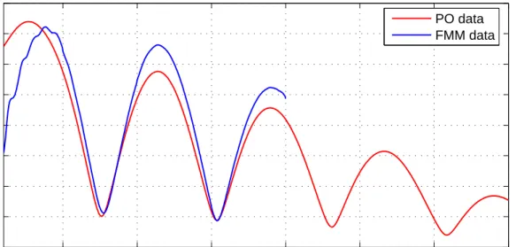
4.1 Comparison of analytical and FMM data. . . 44
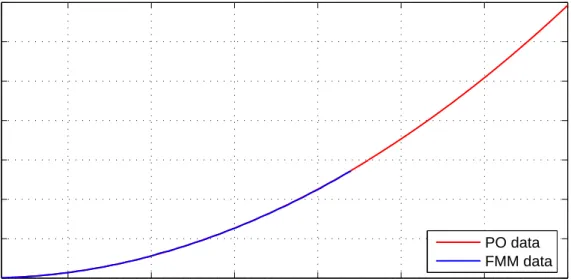
4.2 Comparison of analytical and PO data. . . 45
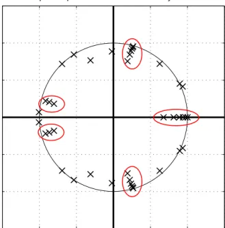
4.3 Distribution of complex exponentials for 1–6 GHz analytical data, M = 40. . . . 48
4.4 Distribution of complex exponentials for 1–4 GHz analytical data, M = 30. . . . 48
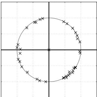
4.5 Distribution of complex exponentials for 1–6 GHz FMM data, M = 40. . . 50
4.6 Distribution of complex exponentials for 10–15 GHz PO data, M = 40. . . 50
4.7 Singular value distribution for 1–6 GHz data, FMM and analytical
data. . . 52
4.8 Maximum interpolation error for 1–6 GHz data, FMM and analyt-ical data. . . 52
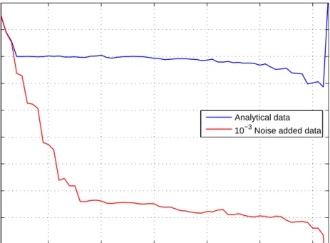
4.9 Singular value distribution for 1–6 GHz data, analytical and noise added data. . . 54
4.10 Maximum interpolation error for 1–6 GHz data, analytical and noise added data. . . 54
4.11 Singular value distribution for 10–15 GHz data, PO data. . . 56
4.12 Maximum interpolation error for 10–15 GHz data, PO data. . . . 56
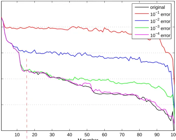
4.13 Maximum interpolation error, original data. . . 58
4.14 Maximum interpolation error, 10−1 noise added data. . . . 58
4.15 Maximum interpolation error, 10−2 noise added data. . . . 59
4.16 Maximum interpolation error, 10−3 noise added data. . . . 59
4.17 Maximum interpolation error, 10−4 noise added data. . . . 59
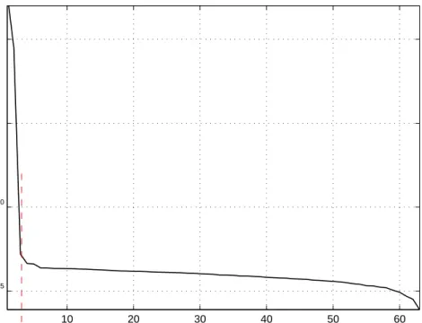
4.18 Maximum interpolation error for different levels of noise added data. 60 4.19 Singular value distribution of patch-over-ring PO data. . . 62
4.20 Backscattering solution signals of patch-over-ring geometry. . . 64
4.21 Backscattering solution signals of rectangular prism geometry. . . 64
4.22 Schematic representation of WCOMPM. . . 65
4.23 Blow up in the FMPM in the FMM solution signal. . . 67
4.25 WFMPM with weighting parameter (1,0). . . 69
4.26 WFMPM with weighting parameter (100,1). . . 69
5.1 Square patch problem. . . 71
5.2 FMM and PO solution data for backscattering square patch problem. 72
5.3 Estimation of noise on FMM and limiting M value for the square patch geometry. M limit is indicated by the vertical dashed line. . 74
5.4 Singular values of PO data and limit for M value. . . . 74
5.5 FMPM extrapolation of 1–8 GHz FMM data, M = 9, (a) signals, (b) errors. . . 75
5.6 BMPM extrapolation of 30–35 GHz PO data, M = 2, (a) signals, (b) errors. . . 76
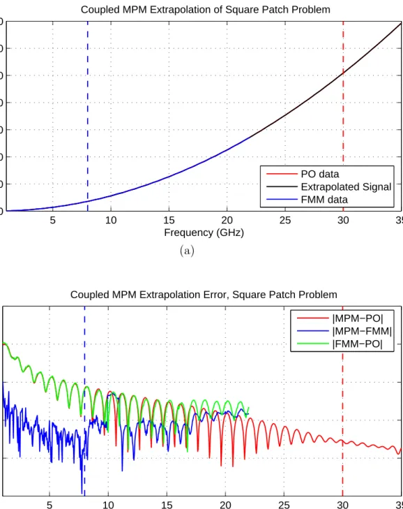
5.7 COMPM extrapolation of 1–8 GHz FMM, 30–35 GHz PO data, (ML, MH) = (9, 2), (a) signals, (b) errors. . . . 77
5.8 CDMPM extrapolation of 1–8 GHz FMM, 30–35 GHz PO data, (ML, MH) = (9, 2), (a) signals, (b) errors. . . . 78
5.9 Patch-over-ring problem. . . 79
5.10 FMM and PO solution data for backscattering patch-over-ring problem. . . 80
5.11 Estimation of noise on FMM and limiting M value for the patch-over-ring geometry. M limit is indicated by the vertical dashed line. . . 82
5.12 Singular values of PO data and limit for M value. . . . 82
5.13 WFMPM extrapolation of 7–15 GHz FMM data, M = 12 and WL= 1000, (a) signals, (b) errors. . . 83
5.14 BMPM extrapolation of 30–35 GHz PO data, M = 4, (a) signals, (b) errors. . . 84
5.15 WCOMPM extrapolation of 7–15 GHz FMM, 30–35 GHz PO data, (ML, MH) = (9, 2) and WR= 4, (a) signals, (b) errors. . . 85
5.16 CDMPM extrapolation of 7–15 GHz FMM, 30–35 GHz PO data, (ML, MH) = (9, 2), WL= 1000, (a) signals, (b) errors. . . 86
5.17 Rectangular prism problem. . . 87
5.18 FMM and PO solution data for backscattering rectangular prism problem. . . 88
5.19 Estimation of noise on FMM and limiting M value for the rectan-gular prism geometry. M limit is indicated by the vertical dashed line. . . 90
5.20 Singular values of PO data and limit for M value. . . . 90
5.21 WFMPM extrapolation of 4–16 GHz FMM data, M = 14 and WL= 1000, (a) signals, (b) errors. . . 91
5.22 BMPM extrapolation of 30–40 GHz PO data, M = 6, (a) signals, (b) errors. . . 92
5.23 WCOMPM extrapolation of 4–16 GHz FMM, 30–40 GHz PO data, (ML, MH) = (14, 4) and WR= 100, (a) signals, (b) errors. . . 93
5.24 CDMPM extrapolation of 4–16 GHz FMM, 30–40 GHz PO data, (ML, MH) = (14, 6), WL = 1000, (a) signals, (b) errors. . . 94
5.25 Bistatic RCS plot of FMM solution, square patch problem. . . 96
5.26 Bistatic RCS plot of PO solution, square patch problem. . . 96
5.28 Error between FMM and PO data for every observation angle and frequency, square patch problem. . . 97
5.29 Error between FMM data and extrapolated signal for every obser-vation angle and frequency, square patch problem. . . 98
5.30 Error between PO data and extrapolated signal for every observa-tion angle and frequency, square patch problem. . . 98
A.1 Sample frequency domain signal. . . 104
3.1 Brute-force optimization results for COMPM . . . 39
Introduction
1.1
Electromagnetic Problems and Their
Solu-tions
Scattering solutions of arbitrarily shaped three-dimensional (3-D) conducting bodies have always been of interest in computational electromagnetics (CEM). There are various applications in which these solutions play crucial roles, such as target identification, military aircraft design, and antenna design. Often, it is important to have the full knowledge of the scatterer’s spectral properties. Accu-rate solvers that calculates the scattering solutions for these problems exist, but these solutions demand more memory and CPU time as the solution frequency increases. These type of solvers perform the same solution procedure for every other solution frequency, but as the frequency increases, resource demands of the solution procedure increase. Therefore, it is usually impossible to obtain the scattering solution on the whole spectrum using these solvers.
On the other hand, as the solution frequency goes to relatively high frequen-cies, the electromagnetic waves start to act under the laws of optics. Using this approximation, it is possible to simplify the solution procedures involving complex interactions and dense matrix operations to algorithms requiring the evaluation
of much simpler expressions. This provides us with a new class of solvers, namely, high-frequency (HF) solvers, which can produce scattering solutions very rapidly. The only drawback of these solvers is their reduced accuracy, which is related to the HF approximations of electromagnetics.
A common approach for accurately solving arbitrarily shaped 3-D bodies is using method of moments (MOM). In order to solve for the scattered field when the target body is illuminated with a plane wave, we first need to discretize the surface of the geometry using small triangles, which is called meshing. A large matrix is filled with the electromagnetic interaction values of these triangular elements. The excitation information is used to fill the right-hand-side vector. The solution of the ensuring matrix equation is the coefficients of the surface current induced on the scatterer. The surface current is then used to calculate the scattered field at any point in space. In order to solve accurately enough, dimensions of each triangle should not be larger than λ/10, where λ corresponds to the wavelength at the specific solution frequency. With a closer look at this procedure, it can be seen that, when the solution frequency increases, i.e., elec-tromagnetic size of the scatterer increases or wavelength decreases, the size of the interaction matrix also increases; hence the solution of that system becomes prohibitively difficult.
Various approaches have been developed such as the fast multipole method (FMM) and its multi-level version, namely, the multi-level fast multiple algorithm (MLFMA), to increase the solution efficiency of the matrix system. A good overview and detailed algorithms for these methods can be found in [1]. A recent trend in CEM is to solve these high-resource demanding problems in parallel computing environments. These improvements to MOM are quite effective in increasing the maximum solvable frequency limit, nevertheless, still a limit exists, albeit higher.
On the other end of the spectrum, with the help of the HF approximations of the electromagnetics, HF solvers do not deal with much of the burden that the low-frequency (LF) solvers face. We use a popular HF solution algorithm, namely, physical optics (PO), to find the scattering solution at relatively high
frequencies. Once again, as in the MOM based solvers, the surface of the scat-terer is discretized using small triangles. Since the electromagnetic waves can be assumed to obey the laws of optics at these frequencies, each triangle on the sur-face of the scatterer is marked as lit or dark, depending on whether it is directly (or indirectly, by multiple reflections) illuminated from the source. Scattered field is then calculated by evaluating a “PO integral” on all lit triangles. To sum up, as opposed to MOM-based solvers, in PO, there is no interaction between the triangles, no dense matrix formation, and no solution of that dense system. Therefore, PO algorithm is extremely fast and can produce scattering solutions practically for every frequency. Because the accuracy of the HF approximations tends to decrease as the frequency decreases, the accuracy of the PO solution also decreases, and thus the solution results at low frequencies is nothing useful.
Even at relatively high frequencies, PO may not produce very accurate re-sults. This is mainly due to the fundamental approximations employed in the HF electromagnetics. In order to correct the solution that is obtained by PO, various correction strategies have been developed. In this thesis, we will use edge/wedge current corrected PO data (POE/POW). In the classical PO theory, scattering and diffraction from wedges and edges are ignored. POE and POW correct this by taking into account the scattering from the induced currents on edges and wedges; however, the inaccuracy problem of the overall solution for low frequencies is still intact.
frequency PO MOM FMM MLFMA Parallel MLFMA limi t of lo w-fr equenc y so lvers accur acy l imit f or P O
no solver available for this region
Figure 1.1: Comparison of numerical solvers over the solution spectrum.
summarizes the general distribution of the available solvers over the solution spectrum and the gap between them that stimulates the research presented in this thesis. In order to obtain the full spectral behavior of a scattering body, we propose using extrapolation techniques to estimate the scattering spectrum for intermediate frequencies. In other words, the purpose of this research and this thesis is to bridge the gap between the LF and HF electromagnetic solvers.
1.2
Model-Based Extrapolation
In order to estimate the solution in the intermediate frequency band, we will use the knowledge of the data at LF and HF, which are obtained from corresponding electromagnetic solvers. Using the known data, an appropriate model will be constructed, and extrapolation will be performed by evaluating that model at the frequencies for which the scattering solution is not available. This approach is called model-based extrapolation [2]-[5]. Instead of the widely used rational-function based modeling, we will use complex-exponential based model as they are more consistent with the characteristics of the scattering signals. The model we will use is basically the sum of weighted complex exponentials,
y (f ) =
M
X
i=1
Riesif. (1.1)
We assume that values of the solution signal y(f ) are specified at N equally spaced points, f = 0, 1, 2, ..., N − 1 [6], and expand the summation in (1.1) to obtain N equations. y (0) = R1+ R2+ · · · + RM, y (1) = R1es1 + R2es2 + · · · + RMesM, y (2) = R1e2s1 + R2e2s2 + · · · + RMe2sM, (1.2) ... y (N − 1) = R1e(N −1)s1 + R2e(N −1)s2 + · · · + RMe(N −1)sM.
This system of N equations defines the projection of the solution signal y(f ) onto an M dimensional space that is spanned by complex exponential basis. If
we happen to know the exponent set, {si}, the set of equations in (1.2) becomes a
linear system, whose solution is straightforward. However, we also seek the com-plex exponential basis along with the residual set, {Ri}. Simultaneous solution
of both parameters from the samples of the solution signal y(f ) is a nonlinear problem but in most cases linearizing the nonlinear problem gives an equivalent result. The nonlinear problem is discussed in [7]-[9]. There are two popular lin-ear approaches for the solution of (1.1), namely, polynomial method and matrix pencil method (MPM) [10]. The basic difference between the two methods is that the former one is a two-step process, whereas, the latter one is a one-step process. In addition to this computational inefficiency of the polynomial method, it has low tolerance to noise. The comparison of these two methods, their historical perspectives, their computational and statistical efficiencies are discussed by var-ious authors [10],[11]. In this work, due to its noise tolerance and computational efficiency, we use MPM to find the parameters of (1.1). MPM is explained in the next chapter in detail.
After finding the model parameters through either of the methods mentioned above by using the knowledge of y values in the interval f = (0 : f1),
extrap-olation is performed by evaluating (1.1) for values f greater than f1. However,
this approach will under utilize our knowledge of data, as we will be using only some fraction of the available data. Thus, a new extrapolation scheme will be introduced in the third chapter.
In order to test all the extrapolation schemes we used the analytical solution of a conducting sphere. As we have the analytical solution available, we can obtain the scattering data anywhere on the spectrum. This will enable us to compare the extrapolated signal with the actual signal, and thus make some modifications on the proposed extrapolation strategies. During the progress of this research analytical solver for conducting sphere was studied and implemented, but as it is beyond the scope of this thesis, those topics will be skipped. Interested readers are referred to [12] for the theory of the analytical solution of conducting sphere.
The actual scatterers to be solved are of course not limited to conducting sphere. Results using computationally obtained data are demonstrated in Chap-ter 5; but before that we will present problems and possible solutions that arise when working with these computational data in Chapter 4.
Matrix Pencil Method (MPM)
2.1
MPM Theory
Due to the nature of the electromagnetic solvers, we have samples of the scattering solution signal at discrete frequencies. Therefore, we need to discretize the model (1.1) as y [k] = M X i=1 Rizik k = 0, · · · , N − 1, (2.1)
where we used the discretization
y [k] = y (kFs) (2.2)
and
zk
i = esiFsk
= e(αi+jωi)Fsk. (2.3)
In (2.2) and (2.3), Fs represents the sampling interval. In (2.1) the complex
exponential set {zi} and their corresponding residual set {Ri} are the unknowns
to be determined along with the number of exponentials that will be used when constructing the model, i.e., the number M. This parameter M is very important
when performing extrapolation using the model and will be discussed thoroughly in the next section. The method uses a mathematical tool called matrix pencil,
¯
Y2 − λ ¯Y1, (2.4)
where λ corresponds to generalized eigenvalues of (2.4) [13]. [14] constructs [Y1]
and [Y2] using the N samples of y [k] in such a way that λ corresponds to the
complex exponentials in (2.1). Therefore, the solution of λ, which is indeed an eigenvalue problem, becomes equivalent to the solution of the complex exponen-tial set of the model (2.1). ¯Y1 and ¯Y2 are defined in [14] as
¯ Y1 = ¯Z1· ¯R · ¯Z2, (2.5) ¯ Y2 = ¯Z1· ¯R · ¯Z0· ¯Z2, (2.6) where ¯ Z1 = 1 1 · · · 1 z1 z2 · · · zM ... ... ... z1(N −L−1) z2(N −L−1) · · · z(N −L−1)M (N −L)×M , (2.7) ¯ Z2 = 1 z1 · · · z(L−1)1 1 z2 · · · z(L−1)2 ... ... ... 1 zM · · · z(L−1)M M ×L , (2.8) ¯ Z0 = diag [z1, z2, · · · , zM] , (2.9) ¯ R = diag [R1, R2, · · · , RM] . (2.10)
diag in (2.9) and (2.10) represents a diagonal matrix of size M × M. The param-eter L in (2.7) and (2.8) is called pencil paramparam-eter and acts as an upper bound on the possible values on M. If we evaluate (2.5) and (2.6) by using (2.7)–(2.10), we would obtain ¯ Y1 = y [0] y [1] · · · y [L − 1] y [1] y [2] · · · y [L] ... ... ... y [N − L − 1] y [N − L] · · · y [N − 2] (N −L)×L , (2.11)
¯ Y2 = y [1] y [2] · · · y [L] y [2] y [3] · · · y [L + 1] ... ... ... y [N − L] y [N − L + 1] · · · y [N − 1] (N −L)×L . (2.12)
By using (2.5) and (2.6) in (2.4), we get ¯
Y2− λ ¯Y1 = ¯Z1· ¯R · {¯Z0− λ¯I} · ¯Z2. (2.13)
It is showed in [10] that, provided
M ≤ L ≤ N − M, (2.14)
the rank of the matrix pencil defined in (2.4) will reduce by one if λ is equal to one of the diagonal entries of ¯Z0. In other words, λ will be a rank-reducing
number when it is equal to one of the {zi}; which is also equivalent to saying {zi}
are the generalized eigenvalues of the system defined in (2.4).
We construct our eigenvalue problem as ©¯ Y2− λ ¯Y1 ª · vi= 0, (2.15) or equivalently n ¯ Y1†Y¯2− λ¯I o · vi = 0, (2.16)
where {vi} are the eigenvectors of the matrix pencil and ¯I is the identity matrix.
¯
Y1† is defined as the Moore-Penrose pseudoinverse of ¯Y1:
¯ Y1† =©Y¯H 1 · ¯Y1 ª−1 · ¯YH 1, (2.17)
where H denotes conjugate transpose. Often the ¯Y1†· ¯Y2 product produces a bad
conditioned matrix, especially when dealing with noisy data. Total least squares matrix pencil method (TLS–MPM) proposes a new approach to find λ that can be used for noisy data. In TLS–MPM, we combine (2.11) and (2.12) to form the single matrix ¯ Y = y [0] y [1] · · · y [L] y [1] y [2] · · · y [L + 1] ... ... ... y [N − L − 1] y [N − L] · · · y [N − 1] (N −L)×(L+1) , (2.18)
which can be defined in terms of (2.12) and (2.13) as ¯ Y = h c1 Y¯2 i = h ¯ Y1 cL+1 i , (2.19)
where ci represents the ithcolumn of (2.18). We use singular value decomposition
(SVD) approach on (2.18) to filter the singular values that cause bad conditioning. ¯
Y = ¯U · ¯Σ · ¯VH. (2.20)
In (2.20) we can modify ¯V such that ¯
Y1 = ¯U · ¯Σ · ¯VH1, (2.21)
¯
Y2 = ¯U · ¯Σ · ¯VH2, (2.22)
where, ¯V1 is obtained by removing the last row of ¯V and ¯V2 is obtained by
removing the first row of ¯V. We filter the singular values by keeping M of them, which ensures a better condition number. Likewise, we also keep or discard the corresponding columns and rows of ¯U and ¯Σ. This can be represented in MATLAB notation as ¯ U0 = ¯U(:, 1 : M), (2.23) ¯ V0 1 = ¯V1(:, 1 : M), (2.24) ¯ V0 2 = ¯V2(:, 1 : M), (2.25) ¯ Σ0 = ¯Σ(1 : M, 1 : M). (2.26)
By using (2.23)-(2.26), we can rewrite (2.21) and (2.22) as ¯
Y01 = ¯U0· ¯Σ0· ¯V0H1 , (2.27) ¯
Y0
2 = ¯U0· ¯Σ0· ¯V0H2 . (2.28)
After substituting (2.27) and (2.28) back into (2.15), we obtain ©¯
U0· ¯Σ0· ¯V0H
2 − λ ¯U0· ¯Σ0· ¯V0H1
ª
· vi = 0. (2.29)
Left multiplying (2.29) with ¯Σ0−1· ¯U0H will give us
© ¯ V0H 2 − λ ¯V0H1 ª · vi = 0, (2.30)
which follows from the fact that ¯U0 is a unitary matrix and { ¯Σ0−1· ¯U0H· ¯U0· ¯Σ0}
is equal to the identity matrix. If we redefine the eigenvectors as
vi = ¯V01· v0i, (2.31) we will get © ¯ V0H 2 · ¯V01− λ ¯V0H1 · ¯V01 ª · v0 i = 0 (2.32) n¡ ¯ V1]0H · ¯V01 ¢−1 · ¯V0H 2 · ¯V01− λ¯I o · v0 i = 0 (2.33) n¡ ¯ V1]0H · ¯V01 ¢−1 · ¯V0H 2 · ¯V01 o · v0 i = λvi0. (2.34)
The solution of the eigenvalue problem in (2.34) will give the M complex ex-ponentials. Once we determine the complex exponentials we can easily determine the residuals from (2.1) as
y [0] y [1] ... y [N − 1] = 1 1 1 1 z1 z2 · · · zM ... ... ... zN −1 1 zN −12 · · · zMN −1 · R1 R2 ... RM . (2.35)
2.2
Extrapolation Using MPM
frequency f1Figure 2.1: Low frequency part of the typical solution spectrum. Solid line repre-sents the available data from LF solver and dashed line reprerepre-sents the unknown region.
Consider the situation that is illustrated in Figure 2.1, which represents a sample solution signal for the low frequency part of the solution spectrum. In
this figure, solid line represents the known part of the signal, whereas, the dashed line represents the unknown part. Typically, the solid-line part is acquired from an LF solver such as FMM, where f1 represents the maximum solvable frequency for
this specific problem. The maximum solvable frequency depends on the method that is used to solve the problem (MOM, FMM, MLFMA or parallel MLFMA), electromagnetic size of the scatterer, mesh density and physical memory of the computer on which the problem is solved.
MPM, as described in the previous section, is used to find the parameters of the model that is to be constructed from the values of the scattering solution signal up to frequency f1. Afterwards, this model, which is parametric in
fre-quency, will be evaluated for the frequencies that are greater than f1 to calculate
the extrapolated scattering signal.
2.2.1
Forward and Backward Extrapolation
We perform all the computations in discrete frequency domain; hence, instead of using the actual frequency, the model is evaluated for frequency index k. For simplicity, we can assign k = 0 to the lowest frequency on the spectrum and k = N −1 to the maximum solvable frequency assuming that we have N samples in the solution region. Using these N samples MPM produces M complex exponentials and M residuals. The extrapolation is performed by evaluating (2.1) for values of k as we march in the extrapolation region in the increasing frequency direction. We call this procedure, i.e., modeling the LF solution and extrapolating in the increasing frequency direction, forward MPM extrapolation (FMPM).
Similarly, we can also model the HF solution and extrapolate in the decreasing frequency direction. We named this approach as backward MPM extrapolation (BMPM). There are two straightforward ways to perform this extrapolation: The first and simpler one is reversing the signal on the frequency axis so that the highest frequency becomes the lowest frequency with index k = 0 and the lowest frequency whose accuracy is acceptable becomes f1 in Figure 2.1, with index
flipping the signal, FMPM can be applied, but the result of the extrapolation should also be reversed on the frequency axis. Second one is to start the frequency index of the model at k = k2, where k2 corresponds to the starting frequency of
the HF solution, i.e., the lowest frequency whose accuracy is acceptable.
If we look closer to the theory of MPM described in the previous section, it can be observed that as long as the data samples that we construct the model from are same, we would end up with the same complex exponential set. In other words, changing the initial value of frequency index does not alter the complex exponentials. However, it does change the residuals that are associated with those complex exponentials. As a result, the extrapolated signal would be same regardless of the choice of the initial value for the frequency index.
Another remark for the frequency index k is that one should watch out for the behavior of the extrapolated signal at large values of k. As the extrapolation frequency increases, the value of k increases too. Recall that k is the power of the complex exponential in (2.1). If the magnitude of any complex exponential is significantly larger than unity, large values of k will blow the extrapolated signal up. There may also be some numerical errors for very large values of k, “very large” being dependent on the platform of implementation.
Up to this point we have never mentioned the parameter M. This parame-ter is nothing but the number of complex exponentials that is used to construct the model and is actually the key point of constructing an accurate model and performing a good extrapolation. In the next sections, we will investigate this pa-rameter in detail and propose a M selection algorithm to obtain the best possible extrapolation.
2.2.2
The Parameter M
During the modeling and extrapolating process, we have left out mentioning about two very important parameters in MPM. They are pencil parameter L and
number of exponentials M. Recall (2.14) that
M ≤ L ≤ N − M. (2.36)
Although L is an intermediate parameter, it does affect the outcome of complex exponentials very much. When dealing with noisy data, it is always a good idea to consider changing L to seek for a better model. However, for simplicity, throughout this thesis, unless otherwise specified, we took
L = N
2, (2.37)
which in turn gives us
M ≤ N
2. (2.38)
Equation (2.38) also gives the maximum number of exponentials that can be used by using a length-N data. It is obvious that if we have length-N data, i.e., N linear equations like (1.2), we could solve for N number of unknowns; N
2 of
them being the complex exponentials, N
2 of them being corresponding residuals.
As M represents the quantity of terms in the model, it should take integer values. Therefore, considering the case of N being odd, we should rewrite (2.38) as
M ≤ bL
2c, (2.39)
where b c represents the floor operation.
Recall that, summation series like (2.1) tend to become more accurate as the number of terms in the series increases. Taylor series, Mie series and Fourier series are some infinite-length series that could be given as example to support this idea. As we cannot sum infinite terms, eventually we have to stop at some point, where the remaining not-summed terms would be the approximation error. In our work, the best model to represent the solution signal would be obtained by using the maximum possible number of exponentials which is N
2. This may
seem correct when we consider the accuracy of the series summation idea just discussed, however, one should keep in mind that we will use the constructed model to extrapolate the signal, not to regenerate it in the interpolation region, i.e., in the region, where we already know the solution values. Using the max-imum possible number of exponentials indeed models the interpolation region
as perfectly as possible, but evaluating that model for frequencies in the deep extrapolation region will cause a blow-up on the extrapolated signal. The rea-son for this possible blow-up is obvious actually, by using maximum number of exponentials, we optimized our model with respect to the interpolation region and did not care about the extrapolation process. In the next section we will provide an optimization strategy to select a value of M that does “care” for the extrapolation process.
2.2.3
Brute-Force Optimization of M
frequency Figure 2.2: Brute-force M optimization for FMPM extrapolation. Solid line is modeled and extrapolation is performed in the increasing frequency direction. Extrapolation performance is evaluated by comparing extrapolated signal with the dotted line part.
Figure 2.2 illustrates the general situation for the case of FMPM. The LF available data is represented with a solid line, and the HF available data is rep-resented with a dotted line; dashed line represents the unknown region for the solution signal. Usually what we perform in FMPM, is first modeling the part that is represented by solid line and evaluating that model for the rest of the spectrum. However, there are bN
2c different models that we can build using
dif-ferent number of exponentials. Clearly, as discussed in the previous subsection, the approximation accuracy of the solid-line region, i.e., interpolation region (IR), increases as the number of exponentials used to create the model increases, but what happens to the extrapolated signal as we increase M?
simple algorithm that scans all possible values of M defined in (2.38). For each possible value of M, a model is formed and extrapolation is performed up to the highest frequency of the spectrum. In order to identify a good extrapolated signal, we compare the error in the dotted-line region, i.e., we find the error between the extrapolated signal and HF available data. The M value that gives the smallest error is selected and used for extrapolation. Since we scan all possible values of M during this optimization approach, we call this procedure brute-force M optimization.
Available HF data gives us a chance to obtain an extrapolation error value, which is in fact invaluable. By using this technique we are minimizing the error in the extrapolation region (ER). The only possible drawback for this approach is the execution speed of the algorithm. Although MPM and extrapolation algorithms require very little CPU time, increasing the sample number on the data, N, will increase the CPU time of optimization process due to (2.39).
frequency Figure 2.3: Brute-force M optimization for BMPM. Solid line is modeled and extrapolation is performed in the decreasing frequency direction. Extrapolation performance is evaluated by comparing extrapolated signal with the dotted line part.
In a similar sense we can apply this optimization to BMPM. Figure 2.3 illus-trates the spectrum for the backward case. In this figure solid line represents the HF available data, dotted line represents the LF available data and dashed line again represents the unknown region. The optimization procedure is same but reversed.
opposite ends of the spectrum is really a chance, but not absolutely necessary to perform an M optimization. In the case of single data source availability, e.g., only LF data, we can spare some solution data at the end of the solution region and model the rest. A similar M scan could be performed but this time instead of finding the error at the other end of the spectrum, we use the spared data to find the error at the beginning of the extrapolation region. When compared, using the error on the other end of the spectrum is clearly a better idea than the latter one.
2.3
Scattering from a Conducting Sphere
Figure 2.4: Conducting sphere illuminated from its south pole.
Up to this point we have given the theoretical background information for MPM, FMPM, BMPM, and brute-force M optimization. In this section, we will present some extrapolation examples that are end products of these methods. We will use backscattering radar cross section (RCS) of a conducting sphere that is illuminated by a plane wave from its south pole. Figure 2.4 illustrates this
situation graphically. Backscattering RCS is the scattering from the south pole of the sphere, i.e., opposite to the direction of illumination.
We chose conducting sphere because we have implemented an analytical solver for this scattering problem in order to test the proposed extrapolation methods. Detailed theory of this solution is given in [12]. In the scattering solution of a sphere, all electromagnetic quantities are expressed as infinite summation of spherical harmonics, which is called Mie series. As we can not operate on infinite number of terms, an iterative technique is used to determine the number of terms to be used in the series for an externally given error criteria. Reflected field from the surface of the conducting sphere is derived analytically using the incident field and boundary conditions are enforced on the surface of the sphere. After finding the required number of spherical harmonics to be used in the expansion, the scattered far-field is calculated by simply evaluating the series. Thus, using this analytical solver we can obtain scattering value of conducting sphere at any frequency easily, in a way, before starting extrapolation we already know the signal on the whole spectrum.
0 1 2 3 4 5 6 7 8 9 10 0 0.5 1 1.5 2 2.5 3 3.5 4 Frequency (GHz) Normalized backscattering RCS ( σ / π a 2 )
The knowledge of the scattering signal over the whole spectrum gives us the chance to test the accuracy of the proposed extrapolation methods. During the testing process, we will restrict our knowledge of the scattering signal to the relevant LF and HF region intervals, forming a situation similar to Figure 2.2 or 2.3. The performance of the extrapolation will be evaluated by comparing the extrapolated data and the previously obtained analytical data in the ER. The backscattering signal that will be used is illustrated in Figure 2.5. This signal is a well-known signature of the conducting sphere and is widely used to test the proposed methods and improvements in CEM. The RCS values, σ, are normalized with the geometric cross section of the sphere, πa2, hence the signal goes to unity
with oscillations of decreasing magnitude. This is actually expected because as we increase the frequency, the electromagnetic waves act more like light, and at very high frequencies RCS, i.e., what radar sees, becomes equivalent to what we see with our own eyes: the cross section of the sphere.
In Figure 2.5 we only represent the first 10 GHz of the signal, but during the extrapolation process, we used the interval [1:35] GHz. Because very-low frequency scattering solutions can have high oscillations that can degrade the performance of the modeling, we dismiss that region and start our solution signal from 1 GHz. Besides, for the purpose of extrapolation, generally scattering values whose frequency is smaller than 1 GHz are irrelevant. In the next section we will demonstrate the results of FMPM.
2.3.1
Sphere Results with FMPM
In order to test the extrapolation methods, we first select the LF and HF intervals. We make this selection as realistic as possible by keeping the limitations of actual numerical solvers in mind. For the backscattering RCS signal of the conducting sphere, we choose 1–5 GHz region as LF region and 25–35 GHz region as HF data. We used a 0.04 GHz frequency sampling when obtaining solution signal from analytical solver, therefore, we have 101 LF data points and 251 HF data points.
1 5 10 15 20 25 28 30 35 40 45 50 10−4 10−3 10−2 10−1 100 101 102 103 104 M
Maximum Extrapolation Error
Forward MPM M scan
Figure 2.6: Results of brute-force M optimization for FMPM.
Figure 2.6 illustrates the results of the brute-force M optimization. Recall that in FMPM we model the LF data, in this case 1–5 GHz region, and perform extrapolation up to 35 GHz. The extrapolation error is the difference between the extrapolated signal and the HF data. Hence, the error levels in Figure 2.6 corresponds to the maximum error between the extrapolated data and HF data in the 25–35 GHz region for each value of M.
Notice that, as we discussed earlier, for very large values of M, maximum extrapolation error tends to increase; the error value is even greater than 104 after
M = 40, where it can not fit into the plot. At those values of M, interpolation error is very low, but, it can be clearly seen why it is a bad idea to select those values of M for extrapolation. The minimum of maximum extrapolation errors is achieved at M = 28, which is indicated with a dotted vertical line in the figure.
1 5 10 15 20 25 30 35 10−7 10−6 10−5 10−4 10−3 10−2 10−1 100 Frequency (GHz) Extrapolation Error Forward MPM extrapolation
Figure 2.7: Extrapolation error for FMPM.
In Figure 2.7, we present the extrapolation result using this M value. We only present the error level for each frequency because at these levels of error two signals are almost undistinguishable on the same plot. In this figure, error levels that are below 10−7 are also shown as 10−7, so interpolation error, as expected, is
very low. As we march in the ER, error tends to increase but with a smaller slope as frequency increases. The maximum error at the end of the spectrum is below 10−2, which can also be seen from Figure 2.6. As the original signal converges
to unity as frequency increases, we can conclude that 10−2 corresponds to 1%
2.3.2
Sphere Results with BMPM
In BMPM, we model the HF data, which is between 25–35 GHz, and extrapolate in the decreasing frequency direction. In the sphere problem HF data has 251 data points, which means maximum value of M is 125, according to (2.39).
1 20 40 60 80 95 100 125 10−3 10−2 10−1 100 101 M
Maximum Extrapolation Error
Backward MPM M scan
Figure 2.8: Results of brute-force M optimization for BMPM.
Figure 2.8 illustrates the brute-force M optimization results. Each error level in this figure is calculated as the maximum value of difference between the extrap-olated signal and LF data. Minimum of maximum extrapolation errors occurs at M = 95, which is indicated by a dotted vertical line in the figure. When we compare Figures 2.6 and 2.8, it can be seen that, in BMPM case, maximum extrapolation error does not blow up for very large values M. The reason for this difference arises from the way we perform the BMPM. If we happen to reverse the signal, as discussed in the previous section, this figure will look similar to
Figure 2.6; however, we select the initial k index of the model without changing the original frequency-index assignment. Therefore, k values starts from 601 in the model (2.1) and in the system (2.35), where k = 601 corresponds to 25 GHz when spectrum starts from 1 GHz and increments with 0.04 GHz. By doing so, we, in a way, prevent the extrapolated signal to blow up.
1 5 10 15 20 25 30 35 10−7 10−6 10−5 10−4 10−3 10−2 10−1 100 Frequency (GHz) Extrapolation Error Backward MPM extrapolation
Figure 2.9: Extrapolation error for BMPM.
Using the result of brute-force M optimization, we construct the model with 95 exponentials and perform extrapolation in the decreasing frequency direction. Once again we only present the error values for each frequency in Figure 2.9 due to the same reasoning as in the FMPM case. Similarly, the error is very small in the IR and tends to increase as we march in the ER. Maximum error for BMPM turns out to be smaller than 2 × 10⁻¹, which corresponds to 20% maximum error.
When we look closely at Figures 2.6 and 2.8, it can be realized that, the automatic selection of minimum value for maximum extrapolation errors is indeed
the absolute minimum. However, there are plenty of other possible values of M such that the maximum error is very close to the absolute minimum. For example, in the BMPM case there is no need to take 95 exponentials to construct the model, only 5–10 will be enough and will give very close extrapolation results. This concept will be revisited when we introduce the techniques that are used to model computational data in Chapter 4.
Coupled Extrapolation
3.1
Reasons for Coupling
In the previous chapter we discussed the basic extrapolation strategies: FMPM and BMPM. The results of these extrapolation strategies were tested on the conducting sphere problem. These results seem promising, especially FMPM case, where maximum error is less than 1%. However, even the idea of under-utilizing the available data during modeling is enough to seek for some improvements on these extrapolation strategies.
At the end of the extrapolation results in the previous chapter, we have two separate extrapolated signals that are obtained from different models. Among those two extrapolated signals one can not simply identify one as the better one. In the regions where FMPM signal has high error levels, BMPM signal has very low error levels and vice versa. Therefore, after looking at this general picture, we start to seek some way to combine these two signals into one and came up with two different methods. In the next section, Coupled Matrix Pencil Method (COMPM), a modification to original MPM will be presented. Later, we will present the Coupled Deconvolution Matrix Pencil Method (CDMPM), a signal processing approach to combine the two signals. At the end of the chapter, we once again present the results of these two proposed methods on conducting
sphere problem.
3.2
Coupling the Models - COMPM
Using either FMPM or BMPM approach causes an under utilization of the infor-mation we have about the scattering signal. In the FMPM case we only model the LF data without considering the behavior of the HF data. Although we use the HF data in the brute-force M optimization, it still does not affect the model and its parameters. As discussed in Section 2.2.3, using the HF data is not so crucial to find an appropriate M in FMPM; we can also spare some data from the LF data and use it as the reference data. Therefore, having an HF data region is not a necessity when performing FMPM. For BMPM we have a similar argu-ment, where we only model the HF data and the LF data is used only to select an appropriate M value. However, as we do have extra data we should use it to improve the quality of the model and reduce the error levels on the extrapolated signal.
Our first proposal is to couple the two models. Instead of constructing two separate models to extrapolate the same signal, we form a single model and obtain a single extrapolated signal. We call this approach COMPM. First, we need to synchronize the k indexes of the two separate data so that, while constructing the single model for both data sources we have an absolute k index. Synchronizing means, the LF data starts with an index of k = 0 and ends with the index k = k1 = N1, the HF data starts with an index of k = k2 = N2 and ends with
k = N − 1, assuming that whole spectrum is represented with N samples. k1
and k2 corresponds to the highest and lowest frequencies of LF and HF data
respectively. The general picture would look as follows: we have a scattering signal with N samples but we only have the values of NL+ NH samples, rest will
be estimated with extrapolation; here NL and NH are the LF and HF data point
We obtain two complex exponential sets using the procedure described in Sec-tion 2.1 for two separate data sources, {zLi} and {zHi}. This process is performed
independently. After finding these two sets of complex exponentials, we construct a matrix equation similar to (2.35), but this time we use both exponential sets;
y [0] y [1] ... y [N1] y [N2] ... y [N−1] = 1 1 · · · 1 1 1 · · · 1 zL1 zL2 · · · zLML zH1 zH2 · · · zHMH ... ... ... ... ... ... zN1 L1 zL2N1 · · · zLMN1L z N1 H1 zH2N1 · · · zHMN1 H zN2 L1 zL2N2 · · · zLMN2L z N2 H1 zH2N2 · · · zHMN2 H ... ... ... ... ... ... zL1N −1 zL2N −1 · · · zLMN −1L zH1N −1 zH2N −1 · · · zHMN −1H · R1 R2 ... RML+MH , (3.1)
where ML and MH are the number of complex exponentials that are obtained
from LF and HF data respectively. Notice that in (3.1), the two sets of complex exponentials are arranged side-by-side. This enforces the model to use both complex exponential sets for each point on the scattering signal, i.e., we are using both complex exponential sets from LF and HF regions to model the LF region, as well as HF region. The left hand side of (3.1) has a discontinuity on k index, where we simply cascaded all of the known data. Solution of (3.1) will result in ML+ MH coupled residuals, hence completing the coupled model.
Extrapolation is performed by evaluating (2.1) for coupled complex exponen-tials and coupled residuals. As a result of extrapolation, a single extrapolated signal is obtained. Equation (3.1) is also a least squares problem like (2.35) and solution of residuals is in a way fitting the model to the signal y as much as possible; but as we couple the two data sources in (3.1), the fitting treats both data sources equally and tries to estimate the signal y in its LF and HF regions as much as possible. The flowchart that summarizes COMPM is presented in Fig-ure 3.1. Next, we will discuss the modifications that we should do on brute-force M optimization to use with COMPM.
Matrix Pencil Method [0 : 1] y k L M {RLi} {zLi} Matrix Pencil Method [ 2 : 1] y k N − H M {RHi } {zHi } dismiss dismiss Combine
Couple the Models Using Eq. (3.1) {zLi,zHi} {RC }, coupled residuals [0 : 1] y k [ 2 : 1] y k N −
3.2.1
Brute-Force Optimization for COMPM
We discussed the brute-force optimization for FMPM and BMPM in Section 2.2.3. In COMPM, we once again need to select number of complex exponentials that will be used when constructing the model; however, this time we have two degrees of freedom, i.e., two M numbers to select, one for the LF data and one for the HF data. Although finding the complex exponential set for these two separate data sources is an independent process, they form a single model. Therefore, we need to perform a two-dimensional optimization and find an M pair that is good for extrapolation.
In brute-force optimization for COMPM, we scan all possible values of MLand
MH under the constraints of (2.39) using NL and NH. For each pair of (ML,MH),
coupled residuals are calculated and the coupled model is constructed. This model is then used to calculate the extrapolated signal over the entire spectrum. The maximum error in the interpolation region is stored in a matrix, whose location is associated with a (ML,MH) pair. We have to use the IR as the reference data
because we have used all the data available to us. Similar to the one-dimensional case, we can spare some data from the end of the LF available data and the beginning of the HF data, however, this would decrease the amount of data we would use when constructing the model. Whatever the reference data is chosen as, we select the best M pair by locating the minimum value in the error matrix.
3.3
Coupling the Signals - CDMPM
In the previous section we perform extrapolation by coupling the models, i.e., we couple the model parameters. However, in this section we directly use the extrapolation results that we present in Section 2.3 and apply signal processing techniques on those two extrapolated signals to produce one, coupled extrapolated signal. We refer to this process as CDMPM as we make use of the deconvolution operation.
The main motivation for coupling the signals is the low error levels of FMPM and BMPM at the beginning of the extrapolation region. We will use weighting windows for each signal such that the influence of FMPM signal would be high relative to BMPM right after k = k1; and relatively low right before k = k2. This
way, coupled extrapolated signal would be affected by FMPM or BMPM signal more than other at the regions where the error levels are lower than the other extrapolated signal.
Notice that, in CDMPM, we do not alter the complex exponentials or their residuals. These model parameters are directly taken from the model that is used to perform FMPM and BMPM. Likewise, number of exponentials that we should use when constructing the models are selected according to the procedure that is discussed in Section 2.2.3. Therefore there is no need to alter the brute-force optimization as we did in COMPM. Next, we will present the basics of deconvolution operation in discrete domain and carry on with the description of coupled deconvolution process.
3.3.1
Deconvolution in Discrete Domain
Deconvolution is simply defined as undoing what convolution does. It is a well known property in signal processing that convolution in time domain corresponds to multiplication in the Fourier domain [15]; considering two signals x and y and their convolution c in time domain, this property can be represented as
c (t) = F−1{F {x (t)} F {y (t)}} , (3.2)
where, F{ } represents the Fourier transform and convolution is defined as
c (t) = Z ∞
−∞
x (τ ) y (t − τ ) dτ. (3.3)
When we work in discrete domain, we should change our domain transforma-tion tool, i.e., we should use discrete Fourier transform (DFT) instead of contin-uous Fourier transform. We can rewrite (3.2) in discrete domain with x[n] and
y[n] sampled at N points as
c [n] = DFT−1{DFT {x [n]} DFT {y [n]}} . (3.4)
In addition to changing the domain transformation tool, we should also change the convolution operation. In order for (3.4) to be valid, a new type of convolution, circular convolution, should be defined [15]:
c [n] =
N −1X m=0
x [hmiN] y [hn − miN]. (3.5) Equation (3.5) defines an N point circular convolution, where h iN defines a circular shift in a length N sequence. With this set of signals, finding x[n] from known c[n] and y[n] is a circular deconvolution problem. If we rewrite (3.5) in matrix notation as
¯
Y · x = c, (3.6)
we can define the circular deconvolution problem as
x = ¯Y−1· c, (3.7)
where ¯Y is N × N matrix that contains the values of y[n]. For a signal like
y [n] = {a, b, c, d, e} (3.8)
the circular convolution matrix, ¯Y, would be,
¯ Y = a e d c b b a e d c c b a e d d c b a e e d c b a , (3.9)
circularly shifting every column by one. We will use this circular deconvolution operation as a basic building block of coupling in the next section.
3.3.2
Coupled Deconvolution
Assume that Y [k] represents the complete scattering signal in frequency domain. At the beginning of the extrapolation problem, this signal is not available in
complete form; we only have the knowledge of LF and HF regions. We model the LF data between k = 0 and k = k1 and perform extrapolation up to k = N − 1
using FMPM; similarly we model the HF data between k = k2 and k = N − 1
and perform extrapolation down to k = 0 using BMPM. Therefore, we have two estimates of Y [k] in the interval between k = 0 and k = N − 1.
(a) (b) frequency frequency 1 1 0 0 WL WH k 1 k2 N-1 k 1 k2 N-1
Figure 3.2: Truncation windows for (a) FMPM signal (b) BMPM signal.
Consider the two windows presented in Figure 3.2; dotted vertical lines sep-arate LF region, ER and HF region. In the interval k = [0 : k1], i.e., in the LF
region, we keep the value of the window that will be used with FMPM signal unity and value of the window that will be used for BMPM signal zero. This is due to the fact that in this region we already have a solution data and do not want the BMPM signal interfere with it, i.e., we keep the FMPM signal and discard the BMPM one. A similar approach is carried out for the region k = [k2 : N − 1].
This way we ensure that coupling only occurs in the ER, i.e., k = [k1 : k2]. Next
we define two signals in frequency domain, XL[k] and XH[k] as
WH[k] Y2[k] = XH[k]. (3.11)
XL[k] and XH[k] are the truncated versions of Y1[k] and Y2[k] respectively.
Y1[k] and Y2[k] are estimates of Y [k] obtained from FMPM and BMPM.
There-fore, with the knowledge of XL[k] and XH[k] we can write eqs. (3.10) and (3.11)
as
WL[k] Y [k] = XL[k], (3.12)
WH[k] Y [k] = XH[k]. (3.13)
Separate solution of either (3.12) or (3.13) will yield Y1[k] or Y2[k], depending on
the equation solved. However, simultaneous solution of these two equations will lead to a coupled Y [k], a single signal in frequency domain. By using property (3.4), in time domain we can write
xL[n] = wL[n] ⊗ y[n], (3.14)
xH[n] = wH[n] ⊗ y[n], (3.15)
where ⊗ is the N point circular convolution operator, N being the number of samples of y[n]. We can rewrite (3.14) and (3.15) in matrix form as in (3.6):
¯
WL· y = xL, (3.16)
¯
WH· y = xH, (3.17)
where ¯WL and ¯WH are circular convolution matrices of wL[n] and wH[n]
respec-tively. If we combine (3.16) and (3.17) into a single matrix equation, we would
obtain " ¯ WL ¯ WH # · [y] = " xL xL # . (3.18)
Solution of (3.18) is a total least squares problem, which will give the time domain counterpart of the coupled extrapolated signal. In order to obtain the frequency domain coupled signal, we need to apply DFT on the solution of (3.18). Various approaches can be used to solve (3.18), such as singular value decompo-sition or pseudoinverse [16].
W L W H Y k 1 k2 low-frequency solution region
coupling region high-frequency
solution region
k index N-1
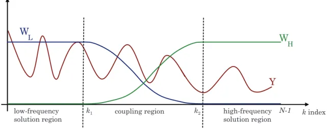
Figure 3.3: Weighting windows used in CDMPM.
Using windows in Figure 3.2 will introduce coupling in the region where both window has value one, i.e., in the ER. However, when the results of Section 2.3 are considered, using rectangular window may not be the best way to perform the coupling operation for MPM-based extrapolation. From the results of Section 2.3 we observe that extrapolation error is low at the beginning of the ER and it increases in the direction of extrapolation. Therefore, it is better to use smooth-transition windows as illustrated in Figure 3.3.
WL[k] and WH[k] in Figure 3.3 become the weighting windows for FMPM
and BMPM signals respectively. We once again use unity and zero weights in the IR. However, in the coupling region, where index is between k = k1 and k = k2,
the weights are adjusted such that at indexes closer to k1, WL[k] is significantly
greater than WH[k], and at the indexes that are closer to k2, WH[k] is significantly
greater than WL[k]; around the center of the coupling region, both weights are
similar.
In Figure 3.4 we illustrate reasons of weight values in each region. Note that, these weights are not weights in the regular sense, but they can still be treated as weights in the sense that we are weighting the coupling process by looking at the extrapolation errors. They are just some windowing functions in frequency domain and they do not have to add-up to unity for each index k. The same coupling procedure will be carried out with these new windows too. The
Frequency
Low-frequency solution region
Coupling region High-frequency solution region Window weight is unity, computational solution is assumed to be correct. Window weight decreases as we march in the coupling region because extrapolation error increases in that direction.
Window weight is zero as we do not need to use the extrapolation signal in this region. We have actual solution from high-frequency solver.
Figure 3.4: Reasoning for weights of FMPM.
flowchart in Figure 3.5 summarizes the CDMPM procedure.
Selection of window type in Figure 3.3 is a study on its own; however, we observed that the widely known window templates such as Blackman–Harris, Hamming, Triangle, Hanning, Chebyshev do not alter the result very much. We choose to use Hanning window throughout this study, without retrying every window for each scattering problem we would like to solve.
Matrix Pencil Method [0 : 1] y k L M Matrix Pencil Method [ 2 : 1] y k N − H M Forward MPM Extrapolation
Couple the Signals Eq. (3.18)
coupled extrapolated signal
{RLi} {zLi} {RHi} {zHi} Backward MPM Extrapolation L W WH Figure 3.5: Flowchart of CDMPM.
3.4
Scattering from a Conducting Sphere
In this section, the results of coupled extrapolation performed on the conducting sphere problem are presented. In order to make a logical comparison with the results presented in Section 2.3, same LF and HF regions are used. First we present the results of COMPM and continue with CDMPM.
3.4.1
Sphere Results with COMPM Extrapolation
A similar choice of regions as in Section 2.3 will lead us to designate 1–5 GHz region as LF region and 25–35 GHz region as HF region. Using a frequency increment of 0.04 GHz we have 101 LF data sample points and 251 HF data sample points. This limits the ML and MH value to 50 and 125 according to
(2.39) respectively.
MH
M L
Maximum Error in the Interpolation Region
1 10 20 30 40 50 60 70 80 90 100 110 120 1 5 10 15 20 25 30 35 40 45 0.0001% 0.001% 0.01% 0.1% 1% 10% 100%
x
i
Figure 3.6: Maximum error in the IR.
We conduct (ML, MH) optimization using brute-force M optimization
dis-cussed in Section 3.2.1. In order to test the effectiveness of this optimization algorithm, we select minimum of maximum errors by looking at both IR error and ER error. In IR error, we fill an ML× MH matrix with maximum error value
between extrapolated signal and the original analytical solution in the IR, i.e., the combination of intervals k = [0 : k1] and k = [k2 : N − 1]. In addition, we also
fill a same size matrix with the maximum error value between extrapolated signal and the original analytical solution in the ER, i.e., in the interval k = [k1, k2]. In
real-life cases, where we do not have the solution signal over the entire spectrum, we only have the IR error matrix, and decide the best (ML, MH) pair accordingly.
M
H M L
Maximum Error in the Extrapolation Region
1 10 20 30 40 50 60 70 80 90 100 110 120 1 5 10 15 20 25 30 35 40 45 0.1% 1% 10% 100%
x
i
Figure 3.7: Maximum error in the ER.
IR and ER error matrices are presented in Figures 3.6 and 3.7 respectively. In these figures x represents the minimum of maximum errors with respect to ER error matrix and i represents the minimum of maximum errors with respect to IR error matrix. They indicate same locations in the two figures; i is the minimum for Figure 3.6 and x is the minimum for Figure 3.7. Notice that IR maximum error values are smaller than those of ER errors in general, which is actually an expected phenomenon. Table 3.1 summarizes the MLand MH values,
the minimum of maximum extrapolation error values for both cases.