CONTENTS
TABLES... ...vii
FIGURES...viii
1.
INTRODUCTION... 1
2.
TOTAL PRODUCTIVE MAINTENANCE (TPM) ... 3
2.1 ASSETCARE ... 4
2.2 MAINTENANCE ... 5
2.2.1 TYPES OF MAINTENANCE ... 5
2.2.2 PREVENTIVE MAINTENANCE (PM) ... 6
2.3 TYPESOFFAILURES... 7
2.4 MEANTIMEBETWEENFAILURES(MTBF): ... 7
2.5 MEANTIMETOREPAIR(MTTR):... 7
2.6 5SPHILOSOPHY... 8
2.7 SINGLEMINUTEEXCHANGEOFDIES(SMED)... 9
2.8 IMPLEMENTINGTPMPRINCIPALS... 9
2.9 DIFFICULTIESOFTPMIMPLEMENTATION ... 12
2.10 TPMACHIEVEMENTS... 13
3
OVERALL EQUIPMENT EFFECTIVENESS (OEE) ... 14
3.1 OEECALCULATION... 16
3.2 OEEINDICATORS ... 18
3.2.1 Availability:... 18
3.2.2 Performance:... 18
3.2.3 Quality: ... 18
3.3 SIXBIGLOSSES ... 19
3.3.1 DEFINITION OF THE LOSSES TYPES ... 20
3.3.1.1 Downtime Losses: ...20
3.3.1.2 Equipment Failures:...20
3.3.1.3 Setup and Adjustments: . ...20
3.3.1.4 Speed Losses : ...20
3.3.1.5 Idling and Minor Stoppages :...20
3.3.1.6 Reduced Speed Operation:...20
3.3.1.7 Defect Losses:...20
3.4 WHYUSEOEE? ... 23
3.5 HOWTOMEASUREOEE? ... 24
4
CASE STUDY... 26
4.1 INTRODUCTIONOFAREVATD ... 26
4.2 PROCESS FLOW: ... 28
4.3 MAINTENANCEPLANNING ... 31
4.4 STRUCTURALLOSSES ... 32
4.5 CAUSEANDEFFECTDIAGRAM ... 32
4.6 IMPROVEMENTONPROGRAMMINGSIDE ... 34
4.7 5SONTHESHOPFLOOR... 36
4.8 DATACOLLECTIONPLAN... 40
4.9 DOWNTIMELOSSESONTHEMACHINE ... 40
4.10 ANALYSINGTHECOLLECTEDDATAS... 45
4.11 PARETODIAGRAMOFTHEDOWNTIMELOSSES ... 49
4.12 STATISTICALANALYSIS ... 51
4.13 OEECALCULATION... 54
5
SUMMARY... 57
REFERENCES ... 58
TABLES
Table 3.1 : Table of six big losses, ...22
Table 3.2 : Myths and realities of OEE ...25
Table 4.1 : Data Collection Form of “Power on Time” & “Program Running Time”...31
Table 4.2 : Data Collection Plan ...38
Table 4.3 : Downtime losses data collection form ...39
Table 4.4 : Main interuptions ...40
Table 4.5 : MWS Output of number of sheets produced...41
Table 4.6 : Comparing Identified and unidentified times ...42
Table 4.7 : Daily Monitoring...43
Table 4.8 : Weekly Monitoring ...44
FIGURES
Fig 2.1 : Workload of types of the maintenance...6
Fig 2.2 : The stages of TPM Implementation ...10
Fig 2.3 : A framework for succesful TPM implementation...11
Fig 2.4 : The roles during TPM implementation ...12
Fig 3.1 : TPM’s pillars...14
Fig 3.2 : OEE Indicators related six big losses and operation times ...17
Fig 3.3 : The types of the losses ...19
Fig 3.4 : OEE Equipment states...23
Fig 4.1 : Picture of PIX Cubicle ...28
Fig 4.2 : Sheet Metal Trolley...28
Fig 4.3 : Process Flow ...28
Fig 4.4 : Detailed Process Flow with additional processes defined. ...29
Fig 4.5 : “Power on Time” & “Program Running Time” data from the machine ...30
Fig 4.6 : Daily and weekly maintenance sheet. ...33
Fig 4.7 : Maintenance Plan, Visual management tool for MTBF ...34
Fig 4.8 : Cause & Effect Diagram ...35
Fig 4.9 : Nesting example...36
Fig 4.10 : Tool drawer. ...37
Fig 4.11 : Identified . Unidentified Losses and program running time graph ...45
Fig 4.12 : Chart of program running time, identified and unidenfied down time. ...46
Fig 4.13 : Downtime losses ...48
Fig 4.14 : Pareto Diagram of all downtime losses...50
Fig 4.15 : Pareto Diagram of downtime losses without structural leakages...50
Fig 4.16 : Trend of output...51
Fig 4.17 : Histogram of all the datas...52
Fig 4.18 : Histogram of the datas...52
Fig 4.19 : Program Running Time by Month ...52
Fig 4.20 : Histogram and Probability plot of the process by year ...53
Fig 4.21: Histogram of Total Operating Time and Total Lost Time by shift and Xbar.R Chart of Total Operating Time and Total Lost Time by shift...54
1.
INTRODUCTION
The Overall Equipment Efficiency (OEE) was originally coming from Japan in 1971. In 1988, when Nakajima introduced TPM in US, this was also including OEE. Since then OEE has been used as a performance indicator of equipment. Overall Equipments Effectiveness (OEE) is a performance measurement system for an equipment, that clearly defines the losses in manufacturing with a continious monitoring system.
OEE is becoming very popular in operations. It is a key performance indicator (KPI) in TPM. OEE is probably the most important tool in the TPM improvement program
The aim of this thesis is using one of the most reliable performance analyzing methods and evaluate the bottlenecks in a dynamic manufacturing system.
In this paper the benefits of using overall equipment efficiency as a manufacturing improvement tool is explained. To do so a thorough the implementation steps and the results of the methodology are discussed with a case study.
Literature study performed including Lean Manufacturing, Total Quality Management (TQM), Total Productive Maintenance (TPM), Preventive Maintenance (PM), 5S, Single Minute Exchange of Die (SMED), Overall Equipment Effectiveness (OEE) and Toyota Production System (TPS).
In chapter two is being mentioned about TPM, the history of TPM and describing asset care and the maintenance types. Also discussed implementation principals of TPM and the difficulties of TPM implementation.
the types of losses. The reason of using OEE is also mentioned in this chapter.
In chapter four we tried to explain the benefits of using overall equipment efficiency (OEE) as a manufacturing improvement tool. Now we will discuss about the implementation steps and the results of the methodology. The case study is done in AREVA TD, Gebze, Turkey
2.
TOTAL PRODUCTIVE MAINTENANCE (TPM)
Total Productive Maintenance’s (TPM) goal is zero breakdown and zero defects. Off course this improves the productivity and reduces cost.According to G. Brar it is “Maintaining and improving the integrity of our production systems through the machines, equipments, processes and employees that add value” (G.S. Brar; Keeping the Wheels turning, 2006) Preventive maintenance was imported from United States in the 1950s to Japan. It is based on periodic servicing and controlling, and replaced by predictive maintenance in the 1980s. TPM should be implemented on a company wide basis, but usually most of the organizations misunderstood the aim, and thought only shop floor people should be involved in it.
TPM is a very efficient way of doing maintenance by the staff of the organization, it is a improvement way in OEE, autonomous maintenance, and formation of maintenance activities. (Brar, 2006)
TPM aims to establish good maintenance practice through the pursuit of
"the five goals of TPM" : (www.superfactory.com, 2008)
a. Improve equipment effectiveness: Defining the losses, which are downtime losses, speed losses and defect losses.
b. Achieve autonomous maintenance: Given at least the
maintenance responsibilities to the people who is operating the equipment.
c. Plan maintenance: Defining the preventive maintenance stages for all equipments and create the standarts of the maintenance conditions.
d. Train all staff in relevant maintenance skills: Define the responsible people of operating and maintaning and train them. TPM focuces on continuous training for the people.
e. Achieve early equipment management: Eliminating the failures by focusing on the root cause of failures of the equipment, and attact as early as possible.
TPM eliminates the losses;
i. Downtime from breakdown and changeover times
ii. Speed losses
iii. Idle times
iv. Quality defects and scrap
The aim must be to measure and monitor all the losses, and try to reduce them. Reducing those losses will be a benefit of organization’s profitability. (Willmott , McCarthy, 2000)
“Unexpected breakdown losses, speed losses, quality defect losses, in which defects lead to reworking or scrapping; and equipment losses from wear and tear on equipment, reducing its durability and productive lifespan. When it comes to equipment, on the shop floor and beyond, organizations typically pursue four techniques for total productive maintenance (TPM): efficient equipment, efective maintenance, mistake proofing (known as poke yoke in lean contexts), and safety management.” (David R Butcher, 2007)
2.1 ASSET CARE
“The means to increase returns on investment are to decrease the operating costs or to increase the turnover of capital. From the physical assets' point of view, these requirements mean a need for dynamic and continual life cycle management, optimal capacity development, higher overall equipment effectiveness, higher reliability and flexibility of physical assets, and lower maintenance costs of production equipment.”
Asset care is about autonomous maintenance and planned preventive maintetance.
The equipment’s users which are the operators should be trained very well for preventive maintenance. They should maintain the asset on daily basis, check, lubricate, replace parts, perform basic repairs and detect the abnormal behouviour of the equipment. (Butcher, 2007)
2.2 MAINTENANCE
SFS-EN 13306 standard defines maintenance as below:
“Maintenance consists of every technical, administrative and management action during the target’s lifecycle the purpose of which is to maintain or improve the target’s ability to perform its task” (SFS-EN 13306, 2001)
2.2.1 TYPES OF MAINTENANCE
There are some types of maintenance as listed below;
1. Corrective: Done as quickly as possible when a failure occurs
2. Preventive: Regular maintenance perform to prevent failures occur.
3. Predictive – With a good analyse of ‘vital signs’, we should take the necessary actions before a failure comes up.
4. Detective – Performed on the devices like fire alarm, smoke detector etc. They just see need a periodic control to see if they are working or not.
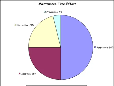
Ia Williamsson catogories the maintenance types as perfective, adaptive, corrective and preventive and showed the work load on those types as in Fig 2.1. (Ia Williamsson, 2006).
Maintenance Time Effort
Perfective; 50%
Adaptive; 25% Corrective; 21%
Preventive; 4%
Perfective Adaptive Corrective Preventive
Fig 2.1 Workload of types of the maintenance; approved by I. Williamsson, 2006
2.2.2 PREVENTIVE MAINTENANCE (PM)
Maintenance of an equipment is recognized as a mandatory action. However, pressures arise from production can result in delaying the scheduled preventive maintenance. Sometimes delay in doing this maintenance is infinite then the equipment breaks down and the maintenance becomes corrective instead of preventive.
The planning should determine how often PM is necessary, what form it should take and which sub-processes should be audited to be sure that PM programming is followed. Maintenance plans are sometimes obliged to be verified based on the data of the Cost of Poor Quality (CoPQ) and high costs incurre due to new investments. Without being in the need of proofing the necessity of PM, the concept total productive maintenance (TPM) is aimed to
use equipment at its maximum effectiveness by eliminating waste and losses caused by equipment malfunctions. (Besterfield, 2003, Juran 1979) Preventive maintenance must be pointed out for controlling the reliability of machines in a process. (Honkanen, 2004)
2.3 TYPES OF FAILURES
Tuomo Honkanen (2004) defined two types of failures in TPM, which are “function-loss breakdowns and function-reduction breakdowns. Function - loss breakdown is a state in which the equipment functioning stops. The function–reduction breakdown is a state in which the machine still operates but causes speed losses and defects”. (Honkanen, 2004)
There is a clear distinction between chronic failures and sudden failures as Nakajima defined (1989). Sudden failures are the ones which are easy to detect and happens randomly, but chronic failures are hidden in production system and happens frequently. Usually the chronic failures happen because of bad conditions such as dirt etc. And TPM’s aim is standardizing the conditions by cleaning and preventing them and keeping operating environment clean and organized by inspecting them. (Honkanen, 2004)
2.4 MEAN TIME BETWEEN FAILURES (MTBF):
Mean Time Between Failures (MTBF) is showing us the equipments reliability. Reliable equipments’ MTBF measurement is high. Usually measured in hours, it can help to quantify the suitability of an equipment for a potential application.
2.5 MEAN TIME TO REPAIRS (MTTR):
“MTTR, or Mean Time to Repairs, is the typical time that a certain device will take to recover from any breakdown.” (http://www.articlewisdom.com Robert Thomson, 2008)
2.6 5S PHILOSOPHY
5S is applied for effective work place organization, reduces waste, simplifies work environment while improving quality and safety.
The five S stand for the five first letters of these Japanese words: 1. “Seiri” means “Sorting out”
2. “Seiton” means “Set in order and Arrange” 3. “Seiso” means “Shine and Sweep”
4. “Seiketsu” means “Standardizing”
5. “Shitsuke” means “Sustain and Self discipline”
One of the important things to do for asset care comes from applying the 5S philosophy.
The aim of applying 5S is getting rid of unnecessary things, putting everything in its right place, keeping the work place clean and organized; and giving the same discipline to everybody. (Willmott , McCarthy 2000) The advantages of implementing 5S in the shop floor are as below;
a. Saving Time,
b. Reduction on the failure ratio, c. Preventing the working accidents,
d. Improvement on productivity and quality, e. Increasing motivation on the employees, f. Improving the employees’ self confidence, g. Increasing competiveness for the company.
Basically 5S process would increase the moral of the employees, increase efficiency. Company becomes competitive in the market with better quality, reaches to faster lead time and less waste, and also it will create positive impressions on customers.
2.7 SINGLE MINUTE EXCHANGE OF DIES (SMED)
“SMED is the term used to represent the Single Minute Exchange of Die or setup time that can be counted in a single digit of minutes. SMED is often
used interchangeably with "quick changeover"” (www.superfactory.com,
2008)
SMED and quick changeover should be used for reducing the time for changing a machine from one product to another.
By applying SMED, we should eliminate non-value added operations, perform external set-up, simplify internal set-up and measure.
2.8 IMPLEMENTING TPM PRINCIPALS
The key of TPM is making it easy to do things right, and difficult to do things wrong.
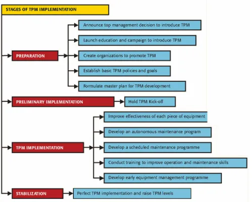
The successful implementation of TPM needs mainly the below stages. (Willmott , McCarthy 2000) (Fig 2.2)
1. Continuous improvement in OEE
2. Operator asset care (autonomous maintenance) 3. Maintainer asset care
4. Quality maintenance
5. Continuous skill development 6. Early equipment management
Fig 2.2 The stages of TPM Implementation; approved by G. S. Brar, 2006
TPM has lots of benefits for the companies. One of the most important benefits is that maintenance expenses are planned and controlled. (Park, Hane; 2001)
In order to develop skills continuously we need to improve people competences to establish the goal of training for sharing ideas, values and behaviors. With this approach the objectives of the training must be linked to business goals, set up a training framework, build capability systematically, design a training and awareness program which encourages practical application to secure skills and future competences.
The supervisors of the company play an important role for implementing TPM. And when the operators involves into the program and knowing their own equipment well, that would help for improvement in the productivity. (Brar, 2006) The concerned people of the program are the operators, team members and managers. It will be structured to maximize the contribution of each individual and to develop their skills to the limit of their capability.
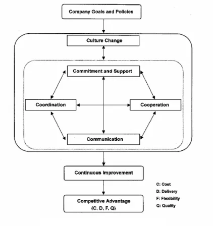
For a successful TPM implementation, companies should setup their strategy first. Understanding TPM philosophy is very important for all level of management. (Fig 2.3) That is a positive culture change in the company, because of that reason communication becomes very important and also HR department’s role is very important for communication.
Decision-making responsibility must be from to the bottom level of the organization up to the top management for a succesful TPM. Everyday a little bit improvement is one of the TPM’s aim.
Fig 2.3 A framework for succesful TPM implementation; approved by K.S. Park, S.W. Hane (2001).
The goal of TPM is improving on operability, maintainability, reliability, product development and service, life cycle cost prediction, feedback and control.
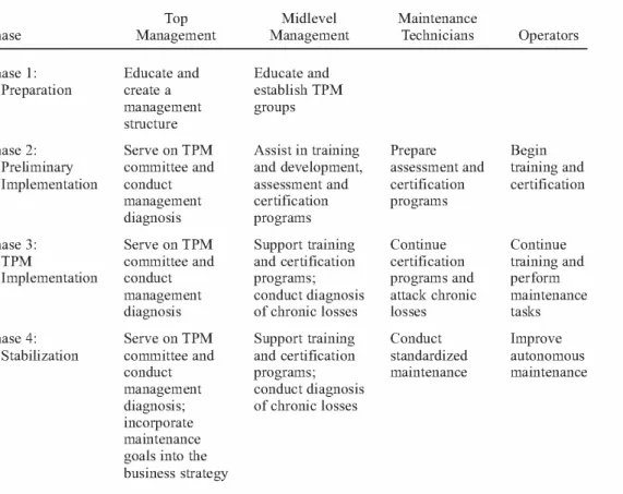
K.S. Park, S.W. Hane (2001) summaries the roles of implementation TPM in
a table very well. (Fig 2.4)
Fig 2.4 The roles during TPM implementation; approved by K.S. Park, S.W. Hane.(2001)
2.9 DIFFICULTIES OF TPM IMPLEMENTATION
We can summaries the difficulties of TPM implementation as following; a. People’s resistance for changings,
b. Not given enough attention, resource etc,
c. Not understanding the philosophy and the methodology well, d. Not being patient enough to see the results, and given up early.
2.10 TPM ACHIEVEMENTS
TPM lets us to improve the progresses in some areas. These are better understanding the equipments performance, equipment importance where it is worth to do improvements on it in order to the potential benefits. TPM improves the teamwork and supports good relationship between production and maintenance. The aim of this work is reducing cost and given better service by improving processes and reducing loss times for example changeovers and setups with trained operators and maintainers. (Brar 2006)
“TPM is one of the world class lean manufacturing strategies that is well structured with eight fundamental development activities and data based approach (OEE) to improve both the effectiveness and efficiency of any production system/process involving everyone”. (ChoyDS; 2003)
TPM adresses excellent manufacturing processes by optimizing the effective use of all manufacturing resources, equipments, people and processes. (Pomorski 1997)
In summary TPM is concerned of improvements in cost, quality and speed and rethinking of business processes.
3.
OVERALL EQUIPMENT EFFECTIVENESS (OEE)
OEE is coming from the philosophy of lean manufacturing, which is based on the work has done by TOYOTA to improve the production system. The aim of lean manufacturing principles are, pull processing, perfect first time quality, zero defects, waste elimination, continious improvement, flexibility and maintaining long term relationship with suppliers. Lean is basicly getting all things right, in right place, in right time, and in right quantity while elimininating waste. (Dransfeld, 2007)The Overall Equipment Efficiency (OEE) was originally coming from Japan in 1971. In 1988, when Nakajima introduced TPM in US he also introduced OEE. Since then OEE is using as a performance indicator of an equipment. (Sheu, 2006). Now OEE is accepted as a main performance indicator. (Muthiah, Huang, 2006)
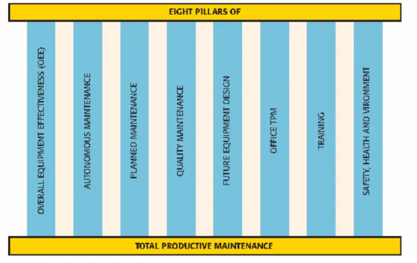
There are eight pillars of TPM as shown in the Fig 3.1: (Brar, 2006). We will focus the first one which is overall equipment efficiency.
“Overall, the TPM implementation leads to an increase in overall equipment effectiveness or availability of machines, increase in productivity, improvement in quality, reduction in inventories, reduction in numbers of accidents, reduced burden on maintenance department and implementation
of scheduled preventive maintenance.” (Brar, 2006)
OEE is probably the most important tool in the TPM improvement program. When the equipment’s productivity is calculated, the time the machine is producing is taking into account, not the amount of the output or the quality. With OEE, those three criteria is taken into consideration, and indicate the all picture of the machine. (Brandt, Tjärning, 2006)
It is very important to focus on the botlenecks in production for increasing the factory’s capacity and productivity. Once all the bottlenecks and losses are defined, then management can focus on the improvements for the impact of efficiency, output and the cost effects of those bottlenecks. (Konopka, Trybula, 1996)
“The best way to increase equipment efficiency is to identify losses that are hindering performance. Moreover OEE is a tool for continous improvement and lean manufacturing initiatives.” (D. R. Butcher; 2007)
For any improvement strategy there must be a way to define and measure how are we doing and how do we compare with the others. (ChoyDS, 2003) Measure of total equipments performance is defined as OEE, which shows us what the equipment is doing and what it is supposed to do. The measurement is based on availability, performance and quality rate of the output. It is based on defining the related equipments losses, which reduce the equipments effectiveness, and improves the assets performance and reliability.
Overall Equipment Efficiency (OEE) measurement can be applied at different levels in manufacturing systems. (Mahadevan, 2004)
a. Measuring initial of manufacturing system and compare with the future values.
b. Points out the bad performances and identify the needs for improvement.
c. The studied and performed line can be used as a benchmark for the other similar facility in the factory.
The methodology categorizes the losses and provides the main areas for improvements priorities and starts with root cause analysis, with this approach it will highlight the hidden capacity. (Muchiri, Pintelon 2007)
OEE’s industrial applications are different from one company to another. OEE is customized for the manufacturer’s industrial requirements.
OEE is a key performance indicator (KPI) in TPM and Lean Manufacturing and it is the best way for monitoring the manufacturing process.
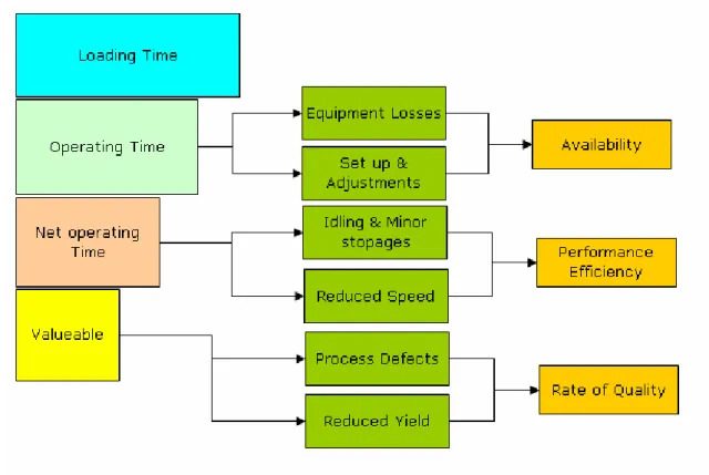
3.1 OEE CALCULATION
Overall Equiment Efficiency is the metric, which Nakajima (1988) used in TPM. It is basically a multiplication of availability efficiency, performance efficiency and quality efficiency. (Giegling et al 1997)
A = ( T/ P ) X 100 = [ ( P- D ) / P ] X 100 A= Availability
T= Total Operating time = ( P- D ) P= Planned operating time
D= Downtime due to equipment failures, setups and adjustment
E = [ ( C X N ) / ( P – D ) ] X 100 E= Perpormance efficiency,
C= Therotical cycle time N= Production amount
R = [ ( N- Q ) / N ] X 100 R= rate of quality products Q= Number of nonconformities
OEE = Availability (A) X Performance (E) X Quality (R) (Besterfield 2004) (Fig 3.2)
Fig 3.2 OEE Indicators related six big losses and operation times; approved by D.H. Besterfield & M. Besterfield, “TQM” 3e, Pearson Prentice Hall, 2003, New Jersey
3.2 OEE INDICATORS
3.2.1 Availability: The equipment’s available time for production, which
was scheduled for. That is the time the equipment is creating value. When it is not doing any value added work due to the failures, breakdowns etc, it is still creating cost. Availability is the ratio of operating time to planned production time.
3.2.2 Performance: Performance is calculated by comparing the actual cycle time against ideal cycle time. Performance is the ratio of net operating time to operating time.
3.2.3 Quality: When the production is wasted and not meet to the
defined quality standarts. It is calculated by comparing the good and reject parts. Quality is the ratio of fully productive time to net operating time.
“The availability rate is determined by three factors, namely reliability, maintainability, and maintenance readiness. The reliability factor is the length of time equipment is able to run without failure and is measured by MTBF. Maintainability is the length of time for which an equipment can be brought back to an operating condition after it has failed, and is measured by MTTR. Since it is the responsibility of maintenance function to ensure the availability of production equipment, the availability rate is related to maintenance effectiveness. The other important time loss is due to changeovers and replacement of routine wear parts.” (P. Muchiri, L Pintelon, 2007)
For TPM implementation Toyota became one of the first company to eliminate the waste (Nakajima, 1988). Toyota defined six categories of equipment losses in its production system, which were equipment failures, setup and adjustments, idling and minor stoppages, reduced speed, defects in the process, and reduced yield (Nakajima, 1986). These six losses are combined into one measure of overall equipment effectiveness (OEE). (Chakravarthy et al 2007)
Even the equipment’s availability is 100 percent, it’s OEE could be extremely low due to the equipment’s performance or to the equipment’s quality of output. (Konopka, Trybula 1996)
There are so many applications in the literature about improving productivity and OEE.
3.3
SIX BIG LOSSES
Nakajima (1988) defines six large equipment losses; (Fig 3.3)
Fig 3.3 The types of the losses
When these six big losses are known then the aim will be focus on these losses, monitor and correct them. That information gives the management and the shop floor people a chance to fix the problem quickly. The aim must be being fast for data collection and categorizing those data. Root Cause Analyzes can be applied for categorizing the data collected. (Korhonen 2007)
3.3.1 DEFINITION OF THE LOSSES TYPES; (Rona, Rooda 2005 and
www.oee.com)
3.3.1.1 Downtime Losses: These are the loss times when machine was planned to run, but it stands still. There is two main types of downtime losses: equipment failures, and setup and adjustments. 3.3.1.2 Equipment Failures: These are the unexpected and sudden
equipment failures, breakdowns. That is the time that the machine is not producing any output. Those losses are categorized as
downtime losses when productivity is less.
3.3.1.3 Setup and Adjustments: This is the time that some machines requires some adjustments ( exp: tool changing ) between
changeovers. That is the time between last good part and the next good part. This is the time that the equipment meet the next requirement of the production, which is time till to the first undefected part.
3.3.1.4 Speed Losses : Speed losses are when the equipment’s running speed is not at its maximum speed as it is designed. There is two types of speed losses: idling and minor stoppages, and reduced speed operation.
3.3.1.5 Idling and Minor Stoppages : These are not technical stopages, usually small problems, which the operator can see and correct. But they could reduce the productivity of the equipment very much. 3.3.1.6 Reduced Speed Operation: This is difference between the
equipments designed speed and it’s actual operating speed. The aim is to reduce the difference between actual and designed speed. 3.3.1.7 Defect Losses: Defect losses mean the equipment’s output is not
meeting the required quality. There is two types of defect losses: scrap and rework, and startup losses.
3.3.1.8 Scrap and Rework: When the equipment’s output is not meeting the specified quality and needs rework to correct the defect. The aim is zero defects and good production at first time.
3.3.1.9 Startup Losses: This is the loss when equipment need time to start-up. Sometimes it can be at an acceptable level, but it could take so much time for stabilization.
Equipment failures and setup and adjustments losses are known as downtime losses and are used to calculate the availability of a machine. The speed losses and idling-minor stoppages are speed losses, which called performance efficiency of a machine. The start up losses and scrap and rework losses are considered to be losses due to defects; the larger the number of defects, the lower the quality rate.
In the below table the losses are very good explained with the examples,
table is from www.oee.com (Table 3.1)
Six Big Loss OEE
Loss Event Examples
Tooling Failures Unplanned Maintenance General Breakdowns Breakdowns Equipment Failure There is flexibility on where to set the threshold
between a Breakdown
(Down Time Loss) and a Small Stop (Speed Loss). Setup/Changeover Material Shortages Operator Shortages Major Adjustments Setup and Adjustments Do w n T im e L o s s Warm-Up Time
This loss is often
addressed through setup time reduction programs.
Obstructed Product Flow Component Jams Misfeeds Sensor Blocked Delivery Blocked Small Stops Cleaning/Checking
Typically only includes
stops that are under five minutes and that do not
require maintenance
personnel.
Rough Running
Under Nameplate Capacity Under Design Capacity Equipment Wear Reduced Speed S p e e d L o s s Operator Inefficiency
Anything that keeps the process from running at its theoretical maximum speed (a.k.a. Ideal Run
Rate or Nameplate Capacity). Scrap Rework In-Process Damage In-Process Expiration Startup Rejects Incorrect Assembly
Rejects during warm-up, startup or other early production. May be due to improper setup, warm-up period, etc. Scrap Rework In-Process Damage In-Process Expiration Production Rejects Q u a li ty L o s s Incorrect Assembly
Rejects during
steady-state production.
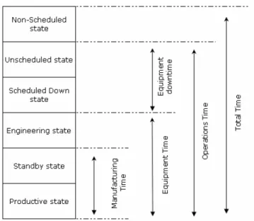
Fig 3.4: OEE Equipment states, approved by De Ron and Rooda
In the Fig 3.4 Rona and Rooda showed the defined six main states of manufacturing equipment. (Rona and Rooda 2005)
3.4 WHY USE OEE?
It is defined by Kaydos as stated in Rona and Rooda (2006) there are five major reasons for companies to measure performance.
1. Improved control, since feedback is essential for any system.
2. Clear responsibilities and objectives. Because good performance measures to clarify who is responsible for specific results or problems.
3. Strategic alignment of objectives. Because performance measures have proven to be a good means of communicating of a company’s strategy through out of the organization.
4. Understanding business processes. Because data measurements require an understanding of the manufacturing process.
5. Determining process capability. Because understanding a process also means knowing it’s capacity.
Overall Equipment Effectiveness (OEE) makes companies to focus improving their equipment’s performance they already own, instead of makes new investments, that means OEE will provide the biggest return on asset
(ROA). (www.downtimecentral.com 2008)
There can be a big improvement on the profitability with small improvements on OEE, 10 percent improvement in OEE can result in a 50 percent improvement in ROA, with OEE is 10 times cost effective than purchasing a new or additional equipment. (Hansen, 2001)
OEE is only given data about the manufacturing processes. The benefit would become obvious, when using OEE with lean manufacturing programms and also as a part of TPM
“An 85 percent OEE is considered as being a world class and a benchmark to be established for a typical manufacturing capability”. (F.K Wang, W. Lee, 2001)
3.5 HOW TO MEASURE OEE?
The most importing thing about measuring OEE is data collection methods. It is the most important state of performance measurement and continious improvement. Data collection can be made manually or automated.
With manuel data collection small stopages and downtimes can be forgotten. Also manuel data collection can demotivate the people, there can be reactions against this measurements. (Muchiri, Pintelon, 2007)
Firstly a data collection plan must be defined and some tools must be created to make the data collection easier for the people, who will be responsible of collection datas. Shop floor meetings must be launch periodicaly. The good ideas are mostly coming from the shop floor people, obviously they are in the middle of the operation and can give good ideas. With this way shop floor meetings will make everybody to involve into the
subject. That makes the people to do things about it, because they are also a part of the decisions which is taken during the meetings.
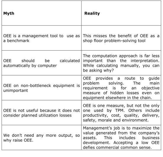
The below table is approved by P. Willmott, D. McCarthy (2000) and shows us the myth and the reality about OEE metric. (Table 3.2)
Myth Reality
OEE is a management tool to use as a benchmark
This misses the benefit of OEE as a shop floor problem-solving tool
OEE should be calculated
automatically by computer
The computation approach is far less important than the interpretation. While calculating manually, you can be asking why?
OEE on non-bottleneck equipment is
unimportant
OEE provides a route to guide
problem solving. The main
requirement is for an objective measure of hidden losses even on equipment elsewhere in the chain.
OEE is not useful because it does not consider planned utilization losses
OEE is one measure, but not the only one used by TPM. Others include productivity, cost, quality, delivery, safety, morale and environment.
We don’t need any more output, so why raise OEE.
Management’s job is to maximize the value generated from the company’s
assets. This includes business
development. Accepting a low OEE defies commercial common sense.
Table 3.2: Myths and realities of OEE, approved by P. Willmott, D. McCarthy, (2000) A Route to World Class Performance
OEE enables the companies to increase their outputs and to discrease the number of defects. There are also some software tools that can be used for measuring, optimizing and implementing OEE for increasing the companies productivity. (Ziemerink, Bodenstein 1998)
4.
CASE STUDY
In this paper we tried to explain the benefits of using overall equipment efficiency (OEE) as a manufacturing improvement tool. Now we will discuss about the implementation steps and the results of the methodology.
The case study is done in AREVA TD, Gebze, Turkey.
4.1 INTRODUCTION OF AREVA TD
AREVA GROUP, world energy expert, offers its customers technological solutions for highly reliable nuclear power generation and electricity transmission and distribution.
65,000 employees are committed to continuous improvement on a daily basis, making sustainable development the focal point of the group’s industrial strategy.
AREVA T&D's leading position in today's energy market follows over 125 years of pioneering innovation, technological expertise and an unwavering commitment to quality and customer service.
AREVA T&D offers solutions to bring electricity from the source onto the power network.
AREVA T&D builds high- and medium-voltage substations and develop technologies to manage power grids worldwide.
AREVA T&D's technologies and expertise ensure higher safety, reliability and capacity of power grids around the world.
AREVA T&D provides a wealth of solutions for the transmission and distribution of electricity worldwide.
With 68 industrial sites and a presence in more than 100 countries, AREVA T&D provides full-fledged solutions to over 30,000 customers in 160
countries around the world. (www.areva.com 2008)
PRIMARY DISTRIBUTION SWITCHGEAR
The Primary distribution network makes the link between High voltage/Medium voltage substations and Secondary Distribution networks, as well as electro-intensive industries and infrastructures.
The case study with OEE has been done with the CNC punching machine which is belongs to AREVA TD, Areva Turkey Medium Voltage Switchgear (ATM) factory, in Gebze, Turkey and produces medium voltage switchgear cabinets. Those cabinet’s sheet metal parts are produced in mechanical workshop. The mechanical workshop will be called as MWS in this paper. ATM produce PIX cubicles in the assembly line and the sheet metal parts of PIX cubicle are produce by MWS, which is ATM’s sheet metal factory. (Fig: 4.1 and Fig 4.2)
Fig 4.1: Picture of PIX Cubicle Fig 4.2: Sheet Metal Trolley
4.2 Process Flow:
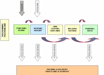
Firstly the process was defined in the workshop; (Fig.4.3).
That was a very simple process map, and should be detailed, and the hidden processes between workstations should be pointed out, also define some necessary processes. In Fig 4.4 is the detailed process map.
Fig 4.4: Detailed Process Flow with additional processes defined.
The study is done on CNC punching machine. The machine was planned to work three shifts a day and six days a week. One shift is 7,5 hours. There is three tea breaks, 10 minutes each and half an hour for lunch break. The time between the shifts is fifteen minutes and the employees are having fifteen minutes for cleaning at end of their shift. The machine is running with a NC program, which is a special software for the machine. Two programmers are working in the programming center.
Some data collection forms were defined at the beginning and see how the machine’s behavior was. Firstly we have defined the time of the machine was having power and the time it was producing physically, which is the time of NC program’s running time. We collect that data directly from the machine. The software which machine uses is able to measure and give us
the exact time. (Fig. 4-5). Machine’s operators should get trained for data collection and they should get understand the importance of those measurement. They had to understand the benefits of this monitoring system, because it is obvious they wouldn’t be pleased to be monitored. If they don’t believe on the benefits of this study, the datas which they would enter would not be very realistic. Each operator were resetting the times before starting their shift, and at end of the shift they were writing down the times on the Data Collection Form 1, (Table 4.1), which was on the screen.
DATA COLLECTION FORM 1
DATE SHIFT OPR H
R M I N POWER ON TIME (MIN) HR M I N PROGRAM RUNNING TIME USAGE % 03.12.07 07:45-15:45 BV 7 56 476 3 10 190 40% 03.12.07 15:45-23:45 AA 7 43 463 3 22 202 44% 04.12.07 23:45-07:45 İK 7 57 477 2 50 170 36% 04.12.07 07:45-15:45 BV 7 35 455 3 7 187 41% 04.12.07 15:45-23:45 AA 7 35 455 3 10 190 42% 05.12.07 23:45-07:45 İK 7 48 468 4 22 262 56% 05.12.07 07:45-15:45 BV 7 40 460 3 0 180 39% 05.12.07 15:45-23:45 AA 6 6 366 2 40 160 44% 06.12.07 23:45-07:45 İK 7 43 463 3 15 195 42% 06.12.07 07:45-15:45 BV 7 41 461 3 21 201 44% 06.12.07 15:45-23:45 AA 7 42 462 4 10 250 54% 07.12.07 23:45-07:45 İK 7 43 463 3 22 202 44% 07.12.07 07:45-15:45 BV 7 56 476 2 55 175 37% 07.12.07 15:45-23:45 AA 7 45 465 3 3 183 39% 08.12.07 23:45-07:45 İK 7 48 468 2 38 158 34% 08.12.07 07:45-15:45 BV 7 40 460 2 51 171 37% 08.12.07 15:45-23:45 AA 7 45 465 3 1 181 39% 09.12.07 23:45-07:45 AA 7 52 472 2 55 175 37%
Table 4.1: Data Collection Form of “Power on Time” & “Program Running Time”
“Power on Time” & “Program Running Time” datas show us the machine was just running 42 percent of the time it was supposed to run, which was not a good result. We had to find the reasons of this big gap.
4.3 MAINTENANCE PLANNING
The operators were responsible of their machines maintenance, we have realised it was not doing with a controlled system and there was some
differences between the operators with the way of doing maintenance. We had to define an exact and proper way for preventive maintetance with the maintenance department.
Firstly we defined all the maintenance steps which operators would be responsible for preventive maintenance which are daily and weekly maintenance tasks. (Fig 4.6). We clocked each task and defined exact rules to do and exact time for them to spend for the maintetance.
A visual management tool was also created to see the breakdowns, electricity cut outs, down air pressure problems and all the planned maintenance on the machine. (Fig 4.7)
4.4 STRUCTURAL LOSSES
There are also some structural losses, which are the tea breaks, lunch breaks, shift changes and cleaning time, which is 20 percent of the time. Those times are certain and we will not work on those.
4.5 CAUSE AND EFFECT DIAGRAM
The next step was defining the hidden losses. We monitored the machine, also make some meetings with the operators about the time they were spending on mostly and the interuptions they were facing during their shifts. With the team members we have defined the cause and effect diagram to see the effects and find out the way of improving the performance of the machine. (Fig. 4.8)
Fig 4.7: Maintenance Plan, Visual management tool for MTBF
4.6 IMPROVEMENT ON PROGRAMMING SIDE
For improvement we need everyone to work on this issue. With this approach we ask to use microjoints on the sheet plate, which is a joint between the parts and the parts are not seperating from the plate while the machine was working. That help us not to stop the machine for collecting the parts on the plate, and the operator were able to do the next job’s preparation, because he was not going and picking up the parts, for every and each time. That helped saving so much time on the machine and the operator’s time. There was other tips we have done on the programming stage which were common punching on the same length edges, nesting in nestings etc. (Fig.4.9) That would make time savings on the machine.
We have done big improvement on the programming side. Now we were ready to work on the operating side.
Fig 4.9: Nesting example
Microjoints were very useful but we have seen the operators was spending so much time on denesting process (breaking the microjoints and collecting the parts from the sheet) , the program was running about 6-7 minutes but denesting was taking about 10-15 minutes, they were also labelling the parts, and this denesting process was done on the machine at that time. It is seen if a seperated denesting table was defined then the operators would run the machine while they were doing denesting on a seperate table. That worked well, and made big improvement on the output.
4.7 5S ON THE SHOP FLOOR
On the punch machines the tool dies are changing between thicknesses, we made a tool cabinet for all the punch and dies, and catagories them. We have put labels on each tool and die, all the tools had identification by this
Nesting in nesting Common punching
way. That help the operators a lot. They were not spending much time for finding the correct tool, and we saved time. Also with this way we have stopped quality defect of using wrong tool and saved also our tools for getting damaged, because wrong tool usage damages the tools, might also breaks them. (Fig. 4.10)
Fig 4.10 Tool drawer.
Damaged tool would produce bad products, which will effect the product quality rate. (Amer 2007)
During the study we have measured the noise level of the punch machine while working, the measurement results were 97 db , which is against the health and safety conditions of the employees even though they are using ear protections. Because of that reason we discussed with the machines producers and found out a way to reduce the noice by reducing the ram speed of the machine. The solution was reducing the cutting force, which reduce the process performance efficiency, but EHS (Employee Health and Safety) is more important then anything else for AREVA TD. After implementing this solution the noise level became below 85 db, which is suitable for the work environment.
The data collection team informed and trained about the importance of this data collection and the way of collecting and entering the datas. (Table 4.2)
P e r io d E v e ry s h if t E v e ry s h if t E v e ry s h if t E v e ry s h if t W e e k ly R e la te d F a c to r s t o R e c o r d # o f s h e e ts M in u te s M in u te s # o f p a rt s d e fe c te d # o f c u b ic le s R e la te d F o r m to r e c o r d T a rg e t s h e e ts P o w e r o n T im e & P ro g ra m R u n n in g T im e E n te ri n g F o rm D o w n T im e E n te ri n g F o rm K K H R ( Qu a li ty C o n tr o l F a il u re E n te ri n g F o rm ) F o rm N o n e H o w m e a s u r e d ? E n d o f th e s h if t th e y m u s t e n te r th e q u a n ti ty o f s h e e t th e y h a v e p u n c h e d D a ta i s c o m in g fr o m th e m a c h in e M a n u a ll y m e a s u re d Qu a li ty c o n tr o l m e a s u re m e n ts P ro je c ts w o rk e d re la te d w e e k R e s p o n s ib le P e r s o n A ll p u n c h in g Op e ra to rs A ll p u n c h in g Op e ra to rs A ll p u n c h in g Op e ra to rs P ro c e s s Qu a li ty P e o p le P ro g ra m m e rs D a ta C o ll e c ti o n D e s c r ip ti o n N u m b e r o f s h e e ts p u n c h e d P o w e r o n T im e & P ro g ra m R u n n in g T im e D o w n T im e L o s s e s D e fe c te d p a rt s N u m b e r o f c u b ic le s p ro d u c e d I te m 1 2 3 4 5
Table 4.2: Data Collection Plan
We have done several shop floor meetings and defined another data collection form and asked them to fill all the losses they are facing. There was 15 tasks, which usually interups the operators while working. The goal of that defining the biggest loss and making improvent on it. (Table 4.3 and Table 4.4)
4.8 DATA COLLECTION PLAN
The most important thing with data collection was actually making everybody to understand the reason of collecting data, otherwise it would not be possible to get reliable datas. Nobody would like to be monitored while working.
4.9 DOWNTIME LOSSES ON THE MACHINE
DT Code DT Description
1001 Tool Setup
1002 Training
1003 Lack of Forklift Driver
1004 Emptying small scrap bin
1005 Emptying big scrap bin
1006 Looking for right size of small plate
1007 Labelling
1008 Checking the tools (takeover the shift)
1009 Looking for a place for the stock parts
1010 Lack of place or trolley for punched parts
1011 Electricity
1012 Breakdown
1013 Air pressure
1014 Lack of program or programming mistakes
1015 Others
Table 4.4: Main interuptions
Table 4.5 is an example for the operators output and target sheet, during the study the target revised 6 times after and each improvement. We used the number of sheets output for calculating the loading and unloading downtime. Obviously as much as the output increase the productivity will get higher. But we have to consider the time of loading and unloading the machine with the raw material.
For calculation we have monitored and take one min for each sheet’s loading and unloading time. This is important to see the time that the operators are spending on the task.
Table 4.5: MWS Output of number of sheets produced.
With this “Failure Data Collection Form” we have defined most of the losses. There was about 40 percent of the lost time was not defined but it went down to 1 percent. (Table 4.6). Which was a big improvent for the beginning but the big issue was making improvements on those losses. Table 4.7 and table 4.8 is shows all the data collected and ready to use for OEE calculation. Table 4.7 is monitored daily datas, and Table 4.8 is monitored weekly summarized data.
Week Power on time (min) Program Running Time (min) Identified DownTime (min) Unindentified DownTime (min) Program Running Time (%) Identified DownTime (%) Unindentified DownTime (%) 49 8735 3600 2441 2694 41% 28% 31% 50 8804 2521 2905 3378 29% 33% 38% 51 4635 1749 1177 1709 38% 25% 37% 52 5561 2076 1399 2086 37% 25% 38% 1 4582 1714 1614 1254 37% 35% 27% 2 9201 3163 2733 3305 34% 30% 36% 3 9280 3123 3099 3058 34% 33% 33% 4 8749 2999 2797 2953 34% 32% 34% 5 3728 1237 1265 1226 33% 34% 33% 6 6019 1916 1775 2328 32% 29% 39% 7 5045 1544 2434 1067 31% 48% 21% 8 6022 2153 1721 2148 36% 29% 36% 9 6959 2562 1856 2541 37% 27% 37% 10 8851 3364 2573 2914 38% 29% 33% 11 7431 2416 3156 1859 33% 42% 25% 12 8426 3114 2210 3102 37% 26% 37% 13 8300 3015 2335 2950 36% 28% 36% 14 7981 2799 2587 2595 35% 32% 33% 15 6027 2644 1761 1622 44% 29% 27% 16 8301 3856 2705 1740 46% 33% 21% 17 6936 3519 2662 755 51% 38% 11% 18 8762 4263 3658 841 49% 42% 10% 19 8833 3907 4674 252 44% 53% 3% 20 8840 3882 4912 46 44% 56% 1% 21 7899 3534 4322 43 45% 55% 1%
4.10 ANALYSING THE COLLECTED DATAS
We realised some petty losses and those were making big changes on the output, for example the operators were downloading the NC programs from the network while machine was stoped, which they can also do while the machine was running. Also they were preparing the tools for the next job when the machine was not working and machine was waiting until the tools get ready and to installing into the machine. We have pushed the operators to do the machine’s adjustment and preparations for the next program while the machine was running. Also some spare cassettes supplied to have the dies ready for different die clearances of the multistations. And more multistations for reducing the time loss on setup. Even those little changes maked improvements and also program running time increased significantly. (Fig: 4.11; Fig: 4.12)
Hrs Analysis 0% 5% 10% 15% 20% 25% 30% 35% 40% 45% 50% 55% 60% 49 51 1 3 5 7 9 11 13 15 17 19 21 Wk %
Program Running Time Identified DownTime Unindentified DownTime
0% 20% 40% 60% 80% 100% 49 51 1 3 5 7 9 11 13 15 17 19 21
Program Running Time Identified DownTime Unindentified DownTime
Fig 4.12: Chart of program running time, identified and unidenfied down time.
During the study there was two big breakdowns happened on the machine, both breakdowns cause was the same, which were the stopage of the conveyer that carries the slugs (small scrap parts) of the sheet. We have put andon lights for the operators, if there is any stopage happens it warns the operator also the rest of the people in the workshop with a red flushing light, if everything is normal and the conveyor works properly it just turn into green light, which was very usefull as a visual management tool. We were confident that there will not be any breakdown because of the same reason. Fig: 4.13 shows us the losses of the machine we have defined during this work.
The main downtime list of the machine is as below; 1. Breaks ( tea breaks and lunch time )
2. Cleaning 3. Shift Change
4. Preventive Maintenance 5. Service
6. Sheet loading and unloading time 7. Tool setup
8. Training
9. Lack of Forklift Driver 10.Emptying big scrap bin 11.Emptying small scrap bin
12.Looking for right size of small plate (cut outs) 13.Labelling the parts
14.Checking the tools ( takeover the shift )
15.Looking for place or trolley for the stock (double bin) parts 16.Looking for place or trolley for the punched parts
17.Electricity
18.Machine breakdown 19.Air pressure
20.Lack of program or programming mistakes 21.Network connection
4.11 PARETO DIAGRAM OF THE DOWNTIME LOSSES
Minitab15 is used for the pareto diagram of the losses. In Fig 4.14 all the losses are seen and Fig 4.15 all the losses without structural leakages are seen, those structural leakages are tea breaks, luch times, cleaning times, shift changes and the time for preventive maintenance. Those times are not planned for any output, those losses are effecting the availability of the machine.
MWS is a supplier of the assembly line and the capacity of the assembly line is about 72 cabinets in a week. At the beginning the machine was producing about 25 cubicles in a week. That shows MWS is just able to produce 34 percent of the line’s capacity, the rest of the sheet metal parts was subcontracting. Because of that reason the improvement of the mechanical workshops capacity was very important for the management, it would also make cost benefits.
The aim was not supplying all the sheet metal work from MWS, it was producing at least 70 percent in house (MWS) and 30 percent outsourced. 70 percent in house makes around 50 cubicle per week. MWS’s weekly target is 50 cubicles. That means 100 percent improvement is accepted from MWS.
After defining all the downtimes, which the operators entered. We have analysed the datas and made a pareto diagram of the losses. Pareto diagrams pointed out the areas we should focus on, from the highest downtime to the lowest one. It seems we should work on loading and unloading time, breakdowns, tool setup and electricity cut offs first.
It was known where to focus with that pareto analysis. And made some changes after defining all the losses, which were some tools, some spare cassets for the dies, a booster for the down air pressure etc. After all those study the output increased significantly. There is still lots of things to do for improvement.
Fig 4.14: Pareto Diagram of all downtime losses
Fig 4.15: Pareto Diagram of downtime losses without structural leakages.
Total (H rs) 397,0 139,0 99,3 99,3 75,2 72,1 60,1 24,7 21,5 19,1 15,8 51,4 P ercent 37,0 12,9 9,2 9,2 7,0 6,7 5,6 2,3 2,0 1,8 1,5 4,8 C um % 37,0 49,9 59,1 68,4 75,4 82,1 87,7 90,0 92,0 93,7 95,2 100,0 S ıra Oth er Lack of p rogr am o r pro gram min g m istak es Lack of F orkl ift D river E lec trici ty T rai ning Tool Set up Pre ven tive Mai nten ance Brea k dow n Shift Cha nge Cle anin g Load ing & U nloa ding Tim e (m in ) Tea Bre ak 1200 1000 800 600 400 200 0 100 80 60 40 20 0 T o ta l (H rs ) P e rc e n t
Trend of the output 0 5 10 15 20 25 30 35 40 45 50 55 60 65 1 3 5 7 9 11 13 15 17 19 21 23 # of cubs produced Linear (# of cubs produced)
Fig 4.16: Trend of output
The benefit of this study is seen obviously in the Fig 4.16. The productivity increased more then 100 percent. MWS’s capacity became above its targets.
4.12 STATISTICAL ANALYSIS
Minitab15 was used for statistical analysis. The below graphs are some statistical analysis of the collected data.
First histogram graph covers all the datas collected during this study, the mean of this period is 182,5 mins, second histogram was made with the data after a few improvements in the process has been done, and the mean of this period is 193,5 mins. And the standart deviation went down from 42,94 mins to 37,99 mins. (Fig 4.17 and Fig 4.18)
280 240 200 160 120 80 40 70 60 50 40 30 20 10 0
PROGRAM RUNNING TIME
Fr e q u e n c y Mean 182,5 StDev 42,94 N 411 Normal
Histogram of Total Operating Time
300 270 240 210 180 150 120 40 30 20 10 0
Total Operating Time
Fr e q u e n c y Mean 193,9 StDev 37,99 N 270 Normal
Histogram of Total Operating Time
Fig 4.17 Histogram of all the datas Fig 4.18 Histogram of the datas collected during the study collected after a few improvements
in the process during the study
320 280 240 200 160 120 80 40 0,018 0,016 0,014 0,012 0,010 0,008 0,006 0,004 0,002 0,000
PROGRAM RUNNING TIME by MONTH
D e n s it y 161 33,88 76 156,4 32,30 48 172,4 24,40 74 209,7 34,20 70 212,5 43,92 81 168,6 46,65 59 Mean StDev N 1 2 3 4 5 12 Month Normal
Histogram of PROGRAM RUNNING TIME by MONTH
Fig 4.19 Program Running Time by Month
We have started to work in December 2007 and in six months time all the statistical analysis proves the improvements. On the Fig 4.19 we see the month of May has the maximum mean then the other months. On the right hand side of the Fig 4.20 are probability plot of the total operating time, right–top probability plot is for all the datas since December Right–bottom probability plot is showing us the difference between the years of 2007 and 2008. In December 2007 datas are very disfuse at the beginning, which is
the time we were just started monitoring and didn’t make many changes on the process. In the Fig 4.21 datas analysed by shifts.
Fig 4.20: Histogram and Probability plot of the process by year
4.13 OEE CALCULATION
Table 4.94: OEE Calculation
Calculating OEE for MWS; (Table 4.9)
1. Preventive Maintenance, Breakdown, electricity cut outs, lack of air pressure times effects the availability of the machine. Which are equipment losses.
For April if we calculate the availability;
A = ( T/ P ) X 100 = [ ( P- D ) / P ] X 100 P = Planned operating time = 38007 min
D = Downtime due to equipment failures, setups and adjustment = = 996min+60min+0 min+135 min= 1191 min
T = Total Operating time = ( P- D ) =38007 min – 1191 min = 36816 min
A = ( T/ P ) X 100 = [ ( P- D ) / P ] X 100 A = (36816 min / 38007 min) X100 = 97% A = 97%
2. Performance efficiency is calculated by # of cubicles that produced into the related week. It is the ratio of produced cubicles and targeted cubicles.
E= Performance efficiency,
C= Therotical cycle time = 242 cubicles was targeted N= Production amount = 210 cubicles was produced E = (210 cub / 242 cub) X 100 = 87%
E = 87%
3. We didn’t take into account the rate of quality, because the detected part percentage was about 0,01% level.
R = [ ( N- Q ) / N ] X 100 R= rate of quality products Q= Number of nonconformities
Defected parts were not taken into account, because the level of defected parts was 0,001 %.
R = 100 %
OEE for April;
OEE = A x E x R = 97% x 87% x 100% = 84%
5.
SUMMARY
In this study Overall Equipment Efficiency (OEE) implementation wasn’t the only way used for increasing the productivity, firstly applying 5S principles on the shop floor minimized the idle time at each process, people had cleaned their workstations and organized work shop. And the motivation effect on the employees was impressive. Implementation 5S helped us to organize the work environment, and give a clear process flow to the
employees, also helped the increase the productivity. During the study we share all the information related the company performance, the workshop’s performance with control chart and graphs on visual display boards. The improvement they see also made them to do better and motivate the people.
The important thing for implementing any improvement method in
companies is to understand the need of total participation of all employees.
MWS had more then 100 percent improvement on the output and choosen as a benchmark sheet metal factory between the Primary Distribution Swithgear (PDS) sheet metal factories in AREVA TD.
REFERENCES
BOOKS
Besterfield D.H. & Besterfield M. , (2003) “TQM” 3e, Pearson Prentice Hall, New Jersey
Hansen R., (2001). OEE for Operators; Shopfloor series.
Juran J. & Godfrey A. B., (1979), ”Juran’s Quality Handbook”, 5e, McGraw-Hill
ARTICLES
Amer W , Grosvenor R , Prickett P., (2007). Machine tool condition monitoring using sweeping filter technologies.
Brandt E. , Tjärning A., (2006). Changing from a Reactive to a Proactive Maintenance Culture; Implementing of OEE.
Brar G. S., (2006). IEE Manufacturer Engineer; February/March . Keeping the Wheels Turning
Butcher D. R., (2007). How to Get Top-Shop Equipment Efficiency
Chakravarthy G. R., Keller P. N., Wheeler B. R., Van Oss S., (2007). A
Methodology for Measuring, Reporting, Navigating, and Analyzing Overall Equipment Productivity (OEP)
ChoyDS S. Y., (2003) . TPM Implementation Experiences
De Rona A. J. , Rooda J. E., (2005). Equipment Effectiveness: OEE Revisited
De Rona A. J. , Rooda J. E., (2006). OEE and equipment effectiveness: an evaluation
Giegling S. ,Verdini W. A., Haymon T , Konopka J., (1997). Implementation of Overall Equipment Effectiveness (OEE) System at a Semiconductor Manufacturer
Honkanen T., (2004). Modeling Industrial maintenance systems and effects of automatic conditions monitoring, ,Helsinki University of Technology
Komonen K., Kortelainen H., Räikkonen M., (2006). An Asset Management
Framework to Improve Longer Term Returns on Investment in the Capital Intensive Industries
Konopka J., Trybula W., (1996). Overall Equipment Effectiveness (OEE) and Cost Measurement
Korhonen J., (2007). OEE (Overall Equipment Effectiveness) and its usage in estimating maintenance performance.
Mahadevan S., (2004). Automated Simulation Analysis of Overall Equipment Effectiveness Metrics
Muchiri, P., Pintelon, L., (2007). Performance measurement using overall equipment effectiveness (OEE): literature review and practical application discussion
Muthiah K.M.N. , Huang S. H., (2006). Overall Throughput Effectiveness (OTE) metric for factory level performance monitoring and bottleneck detection
Park K.S. , Hane S.W., (2001). TPM - Total Productive Maintenance: Impact on Competitiveness and a Framework for Successful Implementation
Pomorski T., (1997). Managing Overall Equipment Effectiveness (OEE) to optimize Factory Performance.
Thomson R. ;www.articlewisdom.com ;(2008). What is MTTR and How Does it Affect You?
Wang F.K. , Lee W., (2001). Learning Curve analysis in Total Productive Maintenance.
Williamsson I., (2006). Total Quality Maintenance (TQMain) A predictive and proactive maintenance concept for software.
Willmott P. , McCarthy D., (2000). Total Productivity Maintenance: A Route to World – Class Performance
Ziemerink R. A. , Bodenstein C. P., (1998). Utilising a LonWorks control network for factory communication to improve overall equipment effectiveness.
OTHER SOURCES www.downtimecentral.com, May 2008 www.oee.com, May 2008 www.superfactory.com, May 2008 www.articlewisdom.com, May 2008 www.areva.com, May 2008
CURRICULUM VITAE
Name Surname : Betül ARSLAN
Address: Şair Arşi cd. No:19 D:19 Göztepe Istanbul Türkiye Date of birth / place : 29.02.1976 / Istanbul
Languages : Turkish (native), English
Primary school : Öğr. Harun Reşit İlkokulu / 1987 Elementary school : Üsküdar Anadolu Lisesi / 1991 High school : Üsküdar Anadolu Lisesi / 1994
BSc : Marmara Üniversitesi / 1998 MSc : Bahçeşehir Üniversitesi / 2008 Name of Institute : Institute of Science
Name of the Program : Industrial Engineering Work Experiences : 08/ 2006 - ... AREVA TD MWS ProductionManager (Kocaeli, Turkey) 07/ 2002 – 08 / 2006 DAT Telekomünikasyon Company Manager (Istanbul, Turkey) 02 / 2001 – 07 / 2002 Makro Danışmanlık CRM Manager (Istanbul, Turkey) 12 / 1998 – 12 / 2000 Principal Group
Purchasing and Foreign Trade Manager (Southampton,UK)