Parallelization of an interior point algorithm for linear programming

?5' I I I I 1 2 F Î M I I I 1 I I 0

r

‘SS6

î T 5 7-^ 4 • 356 Í994

O 2

_i

O 4 9

FOR LINEAR PROGRAMMING

A THESIS SUBMITTED TO

THE DEPARTMENT OF COMPUTER ENGINEERING AND INFORMATION SCIENCE

AND THE INSTITUTE OF ENGINEERING OF BILKENT UNIVERSITY

IN PARTIAL FULFILLM ENT OF THE REQUIREMENTS FOR THE DEGREE OF

M ASTER OF SCIENCE

by

Hüseyin Simitçi July 1994

I certify that I have read this thesis and that in my opinion it is fully adequate, in scope and in quality, as a thesis for the degree of Master of Science.

Asst. Prof. Cevijet Aykanat (Principal Advisor)

I certify that I have read this thesis and that in my opinion it is fully adequate, in scope and in quality, as a thesis for the degree of Master of Science.

Assoc. Prof. Ömer Benli

I certify that I have read this thesis and that in my opinion it is fully adequate, in scope and in quality, as^^-^ll^is for the degree of Master of Science.

Asst. Prof. Kemal Oflazer

Approved by the Institute of Engineering:

__________ __________

P A R A L L E L IZ A T IO N O F

A N IN T E R IO R P O IN T A L G O R IT H M F O R L IN E A R P R O G R A M M IN G

Hüseyin Simitçi

M .S . in Computer Engineering and Information Science Supervisor: Asst. Prof. Cevdet Aykanat

July 1994

In this study, we present the parallelization of Mehrotra’s predictor-corrector interior point algorithm, which is a Karmarkar-type optimization method for linear programming. Computation types needed by the algorithm are identi­ fied and parallel algorithms for each type are presented. The repeated solution o f large symmetric sets of linear equations, which constitutes the major com­ putational effort in Karmarkar-type algorithms, is studied in detail. Several forward and backward solution algorithms are tested, and buffered backward solution algorithm is developed. Heurustic bin-packing algorithms are used to schedule sparse matrix-vector product and factorization operations. Algo­ rithms having the best performance results are used to implement a system to solve linear programs in parallel on multicomputers. Design considerations and implementation details of the system are discussed, and performance results are presented from a number of real problems.

Keywords: Linear Programming, Interior Point Algorithms, Distributed Systems, Parallel Processing.

ÖZET

B İR İÇ N O K T A D O Ğ R U S A L P R O G R A M L A M A A L G O R İT M A S IN IN P A R A L E L L E Ş T İR İL M E S İ

Hüseyin Simitçi

Bilgisayar ve Enformatik Mühendisliği Bölüm ü, Yüksek Lisans Tez Yöneticisi: A sst. Prof. Dr. Cevdet Aykanat

Temmuz 1994

Bu çalışmada, Karmarkar-tipi bir doğrusal programlama optimizasyon algo­ ritması olan Mehrotra’nın predictor-corrector iç nokta algoritmasının paralel­ leştirilmesi sunulmaktadır. Algoritmanın içerdiği işlem tipleri belirlenmiş ve her işlem tipi için paralel algoritmalar sunulmuştur. Karmarkar-tipi algorit­ maların işlem ağırlığını oluşturan büyük simetrik doğrusal denklem kümelerinin çözümü detaylı incelenmiştir. Birçok ileri ve geri çözüm algoritması test e- dilmiş, bir biriktirmeli geri çözüm algoritmeısı geliştirilmiştir. Seyrek matris- vektör çarpımı ve faktorizasyon işlemlerinin dağıtımı için sezgisel bin-packing algoritmaları kullanılmıştır. Performans sonuçları en iyi olan algoritmalar doğrusal programlama problemlerinin çoklu bilgisayarlarda paralel çözümü için bir sistem geliştirilmesinde kullanılmıştır. Dizayn kıstasları ve uygulama de­ tayları tartışılmış, bazı performans sonuçları sunulmuştur.

Anahtar Kelimeler: Doğrusal Programlama, İç Nokta Algoritmaları,

Dağı-tık Sistemler, Paralel İşleme.

I wish to express deep gratitude to my supervisor Asst. Prof. Cevdet Aykanat for his guidance and support during the development of this thesis.

I would also like to thank Assoc. Prof. Ömer Benli and Asst. Prof. Kemal Oflazer for reading and commenting on the thesis.

It is a great pleasure to express my thanks to my family for providing morale support and to all my friends for their invaluable discussions and helps.

Contents

1 Introduction 1

2 Predictor-Corrector Method 5

2.1 Linear Programming P r o b le m ... 5

2.2 Primal-Dual Path Following A lg o r ith m ... 6

2.3 Mehrotra’s Predictor-Corrector M e th o d ... 8

2.4 Predictor-Corrector Interior Point A lgorith m ... 9

2.5 Computation Types for P C I P A ... 10

3 Parallelization of PCIPA 14 3.1 Sparse Matrix-Vector Products ... 16

3.2 Vector Operations... 18

3.3 Sparse Matrix-Matrix P r o d u c t... 19

3.4 Scalar O peration s... 20

3.5 Sparse Linear System S olu tion ... 21

4 Parallel Sparse Cholesky Factorization 23 4.1 Sequential Algorithms ... 23

4.1.1 O rderin g... 25

4.1.2 Symbolic Factorization... 26

4.1.3 Numeric F a cto riza tio n ... 27

4.1.4 Triangular S o lu tio n ... 30

4.2 Parallel A lgorith m s... 30

4.2.1 Ordering and Symbolic F actorization ... 31

4.2.2 Task Partitioning and S ch ed u lin g ... 32

4.2.3 Numeric F a ctoriza tion ... 36

4.2.4 Triangular S o lu tio n ... 39

5 Computational Results for PLOP 61

List of Tables

5.1 Statistics for the NETLIB problems used in this work...54

5.2 Change of factorization times and separator sizes by balance

ratio. (For 16 processors) ... 54

5.3 Change of (FS+BS) times by balance ratio. (For 16 processors) 54

5.4 Computation times and speed-up values for fan-in factorization. 55

5.5 Computation times and speed-up values for fan-in FS (FIFS). . 56

5.6 Computation times and speed-up values for EBFS... 57

5.7 Computation times and speed-up values for EBBS... 58

5.8 Computation times and speed-up values for send-forward BS

(SFBS)... 59

5.9 Computation times and speed-up values for buffered BS (BFBS). 60

5.10 Computation times and speed-up values for the computation of matrix-vector product A 6 ...61 5.11 Computation times (T,in milliseconds), speed-up (S) and per­

cent efficiency (E) values for the computation of matrix-matrix

product A D A ^ ... 62

5.12 Computation times (T,in milliseconds), speed-up (S) and per­ cent efficiency (E) values for one iteration of PCIPA (PLOP). . 63

2.1 The primal-dual path following algorithm... 7

2.2 Variables of PCIPA... 10

2.3 Predictor-corrector interior point algorithm, first part... 12

2.4 Predictor-corrector interior point algorithm, second part... 13

3.1 Algorithm to map rows of A matrix to processors for the mul­ tiplication A S ... 17

3.2 Node algorithm for parallel sparse matrix-vector product AS. 18 3.3 Node algorithm for parallel sparse matrix-vector product A^ip. 18 3.4 Algorithm to construct product sets for each kij... 20

3.5 Node algorithm for the matrix-matrix product A D A ^ ... 20

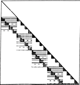
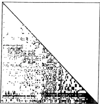
4.1 Nonzero Entries of A D A ^ matrix for woodw problem... 25

4.2 Nonzero Entries of ordered L (factor) matrix for woodw problem. 26 4.3 Sparse column-Cholesky factorization. 28 4.4 Sparse submatrix-Cholesky factorization... 28

4.5 Elimination tree for woodw... 29

4.6 Algorithm for predicting the number of floating-point operations required to generate each column of L ... 33

4.7 Algorithm to generate tree weights... 34

4.8 Task Scheduling Algorithm... 35

4.9 Algorithm to partition the tree... 35

4.10 Fan-in Cholesky factorization algorithm... 37

4.11 Spacetime diagram and utilization count for fan-in factorization of 80bau3b problem... 38

4.12 Node algorithm for EBFS with V = n... 40

4.13 Spacetime diagram and utilization count for EBFS on 80bau3b problem... 41

4.14 Fan-in FS algorithm (FIFS)... 42

4.15 Spacetime diagram and utilization count for fan-in FS on 80bau3b

problem... 43

4.16 Node algorithm for elimination tree based BS (EBBS)... 44

4.17 Spacetime diagram and utilization count for EBBS on 80bau3b problem... 45

4.18 Broadcast BS algorithm... 46

4.19 Send-forward BS (SFBS) algorithm... 46

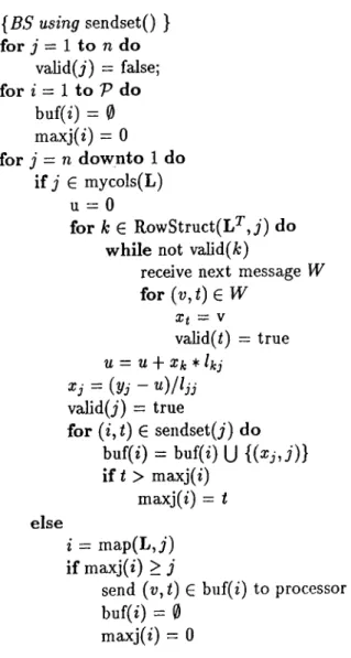
4.20 Buffered BS algorithm (BFBS)... 49

4.21 Spacetime diagram and utilization count for BFBS on 80bau3b problem... 50

5.1 Speed-up curves for fan-in factorization algorithm... 64

5.2 Speed-up curves for FIFS algorithm... 64

5.3 Speed-up curves for EBFS algorithm... 65

5.4 Speed-up curves for EBBS algorithm... 65

5.5 Speed-up curves for SFBS algorithm... 66

5.6 Speed-up curves for BFBS algorithm... 66

5.7 Speed-up curves for matrix-vector product A 6 ... 67

5.8 Speed-up curves for matrix-matrix product A D A ^ ... 67

5.9 Speed-up curves for one iteration of PLOP... 68

Introduction

A consensus is forming that high-end computing will soon be dominated by par­ allel architectures with a large number of processors which offer huge amounts o f computing power. It is inviting to consider harnessing this power to solve difficult optimization problems arising in operations research (OR). Such prob­ lems could involve extending existing models to larger time or space domains, adding stochastic elements to previously deterministic models, integrating pre­ viously separate or weakly-linked models, or simply tackling difficult combina­ torial problems [7]. Another attractive possibility is that of solving in minutes or seconds problems which now take hours or days. Such a capability would allow presently unwieldy models to be run in real time to respond to rapidly changing conditions, and to be used much more freely in “what if” analyses.

The main difficulty is the present lack of sufficiently general parallel sparse linear algebra primitives to permit the wholesale adaptation of existing, proven, continuous optimization methods to parallel architectures.

This work describes the application of highly parallel computing to numer­ ical optimization problems, in particular linear programming which is central to the practice of operations research.

Before getting into details, we should address the question: What is a linear program ? It is an optimization problem in which one wants to min­ imize or maximize a linear function (of a large number of variables) subject to a large number of linear equality and inequality constraints. For exam­ ple, linear programming may be used in manufacturing-production planning

to develop a production schedule that meets demand and workstation capacity constraints, while minimizing production costs. It is being used by the U.S Air Force Military Airlift Command (M AC) to solve critical logistics problems and by commercial air-lines to solve scheduling problems, such as crew planning [4].

Research in linear programming methods has been very active since the discovery of the simplex method by Dantzig in the late 1940’s. It has long been known that the number of iterations required by the simplex method can grow exponentially in the problem dimension in the worst case. More recently, interest in linear programming methods has been rekindled by the discovery of the projective method of Karmarkar, which has been proven to require 0 {n L ) iterations and 0(n^·®) time overall, where T is a measure of the size of the problem, and the claims that variants of this method are much faster than the simplex method in practice [1, 6, 19].

In the past few years, there have been many other interior methods pro­ posed. In this work we will concentrate on the parallel implementation of the one proposed by Mehrotra [18], namely predictor-corrector interior point method.

In general, there is a technical barrier to easy application of parallel com­ puting technology to large-scale OR/optimization models — the lack of suffi­ ciently general, highly parallel sparse linear algebra primitives. If one examines the “standard” algorithms of numerical optimization several critical operations appear repeatedly. Perhaps the most common is the factoring of large sparse matrices, this operation forms the bulk of the work in most Newton-related methods, including interior point methods for linear programming. It is clear that without an efficient parallel version of sparse factoring, it will not be practical to simply “port” existing general-purpose sparse optimization codes to parallel architectures.

CHAPTER 1. INTRODUCTION

2

Previously, most of the research on parallel solution of linear programs concentrated on decomposable linear programs [15, 28], which are assumed to have a block-angular structure. Panwar and Mazumder [25] present a parallel Karmarkar algorithm for orthogonal tree networks. Li et al. [21] give parallel algorithms for simplex and revised simplex algorithms. Currently we are not

aware of any research on the parallelization of interior point algorithms for general linear programming problems on distributed memory message-passing parallel computers.

Distributed memory, message-passing parallel computers, which are usually named as multicomputers, are the most promising general purpose high perfor­ mance computers. Implementation of parallel algorithms on multicomputers requires distribution of data and operations among processors while supplying communication and synchronization through messages. For these architectures it is important to explore these capabilities fully to achieve maximum perfor­ mance. In the following chapters we investigate the efficient parallelization o f the most time-consuming steps of interior point (Karmarkar-type) meth­ ods and elaborate on the methodology used to develop parallel algorithms for these problems. The algorithms and the methodology are used to implement PLOP (Parallel Linear Optimizer), a parallel implementation of Mehrotra’s predictor-corrector interior point algorithm (PCIPA), on iPSC/2 hypercube multicomputer.

In Chapter 2 we will introduce linear programming and PCIPA, and discuss the computation types needed by this algorithm. Parallelization of PCIPA will be discussed in Chapter 3. In this chapter every section will introduce the parallel algorithms for different computation types of PCIPA and how they are implemented in PLOP.

As noted earlier, the main computational effort of the Karmarkar-type lin­ ear programming methods involve the repeated solution of large symmetric sets of linear equations. For this reason, algorithms that optimize the PLOP performance for the solution of sparse sets of linear equations are presented separately in Chapter 4. These algorithms involve both Cholesky factorization and forward-and-backward substitution for the solution of linear equations and exploit data locality and concurrency by scheduling the operations among the processors.

Experimental results for PLOP performance obtained from actual runs on linear programs from the NETLIB suite [8] are presented in Chapter 5. These

CHAPTER 1. INTRODUCTION

data represent realistic problems in industry applications ranging from small- scale to large-scale. Finally we derive the conclusions from the earlier discus­ sions in Chapter 6.

Predictor-Corrector Method

2.1

Linear Programming Problem

Linear programming problem is the problem of minimizing (or maximizing) a linear function subject to a finite number of linear constraints and to the con­ dition that all variables must be nonnegative. The function to be optimized in the linear programming problems is called the objective function.

Mathematically, the linear programming problems can be formulated as follows^:

minimize c ‘ x

subject to A x = b, (2-1)

X > 0.

where A is a given m x n matrix and m < n, b is a given m-component right hand side vector, c is a given n-component coeiBcient vector that defines the objective function, and x is an n-component nonnegative unknown vector. Here, m is the number of constraints and n is the number of variables. This linear programming problem is called the primal problem.

Associated with this primal problem is the dual linear program: maximize b^y

subject to A ^ y -f z = c, z > 0 .

(

2

2

^In this work matrices and vectors are denoted by capital bold letters and small bold letters, respectively. Nonbold small letters are used for scalar values.

which we have written in equality form by introducing slack variables z (also called reduced costs).

The linear programming problem is to find the optimal value of the objec­ tive function subject to the linear constraints. The optimization problem arises because the linear equations A x = b is underconstrained, i.e., the coefficient matrix A contains many more columns (variables) than rows (constraints).

Since Karmarkar’s fundamental paper [19] appeared in 1984, many interior point methods for linear programming have been proposed. Among these vari­ ants the primal affine-scaling, dual affine-scaling [2, 24], one-phase primal-dual affine-scaling, and one-phase primal-dual path following methods are the most popular ones.

We focus on one variant — Mehrotra’s predictor-corrector interior point al­ gorithm (PCIPA). But before introducing PCIPA we will describe the one-phase primal-dual path following algorithm (PDPF), which constitutes the theoret­ ical base of PCIPA. In the next section we give a brief review of the PDPF algorithm. For a more detailed description, see [18, 23, 26]. Also [22] gives an informal and intuitive description.

2.2

Primal-Dual Path Following Algorithm

The PDPF algorithm (Fig. 2.1) is motivated by applying the logarithmic bar­ rier function to eliminate the inequality constraints in (2.1) and (2.2).

Fix /i > 0. Let (x^,y^,z^) be a solution to the following system of 2n -f- m (nonlinear) equations in 2n + m unknowns:

CHAPTER 2. PREDICTOR-CORRECTOR METHOD

6

Ax = b, A^y -f- z = c, XZe = //e, (2.3) (2.4) (2.5)

where e denotes the n-vector of ones, and X and Z denote the diagonal matrices

with X and z vectors, on the diagonal, respectively. The first m equations in

(2.3) are part of the primal feasibility requirement and the next n equations in (2.4) are part of the dual feasibility requirement. The last n equations are called //-complementarity.

start with /i > 0, X > 0, z > 0.

while stopping criterion not satisfied do

p = h - Ax; <7 = c — A ^y — z; 7 = /iX“ 'e — Ze; D = X Z “ ^ A y = (A D A ^ )-‘ (AD(<T - 7 ) + p); Az — <j — A ^ A y ; A x - D(7 — Az);

find Op and cxi such that

X > 0 and z > 0 is preserved;

X < - X -f

y y -I- Ay/ttj; z <— z + Az/ttj

Figure 2.1: The primal-dual path following algorithm. Applying Newton’s method to (2.3)-(2.5), we get

A A x = p, nr A A y -f A z = <7, where Z A x -t- X A z = (f>, p = b — A x , rp <7 = c — A y — z, and (

2

6

2

8

If we multiply (2.7) by A X Z “ ^ and then use (2.8) followed by (2.6), we see that

A y = (ADA^")"^(AD(<7 - 7 ) -b p),

where D is the positive definite diagonal matrix satisfying D = X Z " ‘

and

7 = X"i<^ = pX-^e - Ze.

Once A y is known, it is easy to solve for A z and A x ,

A z = <7 — A ^A y

(2.9)

CHAPTER 2. PREDICTOR-CORRECTOR METHOD

and

The desired update is then

A x = D

(7

X <-- X + A x , (2.12)

y ^■ y + A y , (2.1.3)

z <-- z -f A z . (2.14)

However, there is no guarantee that this update will preserve the nonneg­

ativity of X and z, so a shorter step has to be taken to keep x > 0 and z > 0

using ratio tests.

2.3

Mehrotra’s Predictor-Corrector Method

Mehrotra introduces a power series variant of the primal-dual algorithm. The method again uses the logarithmic barrier method to derive the first-order conditions (2.3)-(2.5). Rather than applying Newton’s method to (2.3)-(2.5) to generate correction terms to the current estimate, we substitute the new point into (2.3)-(2.5) directly, yielding

A (x -f- A x ) = b, (2.15)

A ^ ( y - f A y ) - f (z - f - A z ) = c, (2.16)

( X + A X ) ( Z -h A Z )e = /xe, (2.17)

where A X and A Z are diagonal matrices having elements A x and A z , re­ spectively. Simple algebra reduces (2.15)-(2.17) to the equivalent system

A A x = b — A x , (2.18)

A ^ A y - t - A z = c — A ^ y — z, (2.19)

X A z + Z A x = /¿e - X Z e - A X A Z e . (2.20)

The left-hand side of (2.18)-(2.20) is identical to (2.6)-(2.8), while the right- hand side has a distinct difference. There is a non-linear term A X A Z e in the right-hand side of (2.20). To determine a step approximately satisfying (2.18)-(2.20), Mehrotra suggests first solving the defining equations for the primal-dual affine direction:

A A x = b - A x , (2.21)

A ^ A y + A z = c - A ^ y - z, X A z -f Z A x = - X Z e .

(

2

22

These directions are then used in two distinct ways: to approximate the non­ linear terms in the right-hand side of (2.18)-(2.20) and to dynamically estimate

fi. The actual new step A x , A y , A z is then chosen as the solution to

A A x

= b -

The results given in [18] show that the predictor-corrector method almost always reduces the iteration count and usually reduces computation time. Furthermore, as problem size and complexity increase, the improvements in both iteration count and execution time become greater. Thus the predictor- corrector method is a higher-order method that is generally very computation­ ally efficient.

2.4 Predictor-Corrector Interior Point Algo­

rithm

For the implementation of PCIPA, we will consider a more general form of the primal linear problem with the addition of upper bounds and ranges.

minimize c x subject to A x — w = b, X - f t = u, w -f- p = r X , w, t ,p > 0. (2.27)

where u is the upper bound vector, r is range vector, and w , t, p are appropri­ ate slack variables.

CHAPTER 2. PREDICTOR-CORRECTOR METHOD

₁₀

m number of rows (constraints) n

A constraint matrix b c objective function f r ranges i u upper bounds w X primal solution y z dual slacks p

q dual range slacks s

t upper bound slacks v

Pres primal residual (i.e., infeasibility) dres Pobj primal objective value dobj

Ufc shifted upper bounds

number of columns (variables) right-hand side

fixed adjustment to obj. func. lower bounds

primal surpluses dual solution range slacks

dual for upper bound slacks dual for range (w)

dual residual (i.e., infeasibility) dual objective value

(2.28) Figure 2.2: Variables of PCIPA.

follows:

maximize b ‘ y — u ‘ s — r*q subject to A ^ y — s -f z = c,

y -b q - V = 0, s ,q , V, z > 0.

Implementation of Mehrotra’s predictor-corrector method on this form of linear problem results in the predictor-corrector interior point algorithm (PCIPA) given in Figs. 2.3 and 2.4. Linear programming variables used in PCIPA are explained in Fig. 2.2. In this algorithm, a variable with a capital letter, other than A matrix, denotes a diagonal matrix with the corresponding vector on

the diagonal. We use for matrix transpose and for vector transpose.

Issues concerning the construction of an initial solution and an effective stopping rule are studied in the literature in detail [1, 5, 9, 23].

2.5

Computation Types for PCIPA

A study of PCIPA given in Figs. 2.3 and 2.4 reveals that PCIPA has a wealth o f computation types. We will classify them into five general groups:

1. Sparse Matrix-Vector Products. There are two kinds of matrix-vector product. One is the product of an m x n matrix with an n vector (A 6 ), the other is the product of an n x m matrix with an m vector

2. Vector Operations. These operations include dense vector sum (e.g., y -f-q ), difference (e.g., s — z), inner product (e.g., c ‘ x). We can also include diagonal matrix operations in this type because they are simply

treated as vectors. For example Z X ^ is computed as simply element by element division (z ,/x ,) of two vectors z and x.

3. Sparse Matrix-Matrix Product. This involves A D A ^ , which is the prod­ uct of two sparse matrices A and A ^ scaled by the elements of the diag­ onal matrix D.

4. Scalar operations. Besides standard scalar operations, this type involves the search for a minimum or maximum among a list of scalar values. 5. Sparse Linear System Solution. This is where the most of the solution

time is used in PCIPA and involves the solution of a large sparse linear system K x = b, where K is a positive definite matrix. In PCIPA, K appears to be (A D „A ^ -|- D ^ )·

In the next chapter, we will discuss the parallelization of these computa­ tion types in detail. Since our goal is to get a parallel implementation of the PCIPA, we will have a unified approach in the parallelization of these types by considering the interactions among them.

CHAPTER 2. PREDICTOR-CORRECTOR METHOD

₁₂

find an initial solution start with /i > 0;

/ = U

5

Ub = b ‘ b; Uc = c ‘ c;

itr =

0

while itr < iteration-limit do

p = b - A x -J- w; O’ = c - A^y -f- s - z; a = r - w - p ; /3 = y - t - q - v ;

T = Uj - X - t;

Pobj = c‘x -f- / ; Pre3 = >/p‘ p + t‘t -f a «a / (n^ -1-1);

doti = b‘ y - u^s - r‘ q -f- / ; = ^o-'cr -|- /3^/3 / (wc -f-

1

if stopping-rule()

optimal found; break;

D „ = (ZX -^ -I- S T -» )-^ = (Y W - i -H Q P - i ) - '; 7z = -z ; 7«; = -w ; 7< = - t ; 7 , = -q ; o- = - 7^; p = p + 7u,; = "T - 7«; « = a - 7u,; /3 = /3 - 7 ,; A y = (A D „A ^ + D rn)-\p + D „ ( Q P - 'a - (3) + AD„(<r - S T " V )); A x = D „(A ^ A y - <r -I- S T “ V ); A s = S (A x - r)T "^ e; A p = D ^ (A y -

1

7

7

7

7

o:p = m axi{l, ¿|^m in{A x,/x„ A w ./w ,, At,/t,·, A p ,/p ,} } ;

ad - m ax,{l, ¿ ^ m in {A z ,/z ,, A y ,/y ,, As,/s,·, Aq,/q,·, A v ,/v ,} } ; Op = m ax{l, Op, qj};

IJ. = (

2

20

2

2

7

7

7

A y = (A D „A 3’ + D ^ )-* (p -(- D ^ (Q P -* a - y3) -t- AD„(<r - S T “ *r)); A x = D „(A ^ A y - <r -l· S T “ *r);

A s = S (A x - r ) T “ *e; A p = D ^ (A y -|- V W “ *a -

1

A v = V W “ *(A y - Q P -* a + /3);

A z = 7^ - Z X “ * Ax; A w = 7^ „ - W V “ * Av;

A t =

7

7

t t p = m ax,{l, ¿^ m m {A xj/x,·, Aw,/w,·, At,/t,·, A p j/p ,·}};

arf = m ax,{l, ^ m iii{A z ,/z ,·, Ay^/y,·, As,/s,·, Aqi/q,·, A v ,/v ,·}}; if ((c* A x < 0) and («p = 0) and (pres < 10~^))

primal unbounded; exit;

if ((b*Ay <

0

0

10

dual unbounded; exit;

if (o!p <

1

1

1

1

w = w + Aw/ttp; x = x + A x /a p ; y = y + A y/od ; z = z-|-Az/ad; s = s -f-A s /a j; t = t-(-A t/a p ; v = v-| -A v/od; p = p + A p /a p ; q = q -l-A q /ad ; b = b -I- A£;

X = X -f

Chapter 3

Parallelization of PCIPA

The purpose of this chapter is to investigate the efficient parallelization of PCIPA on medium-to-coarse grain multicomputers. These architectures have the nice scalability feature due to the lack of shared resources and increasing communication bandwidth with increasing number of processors. In multicom­ puters, processors have neither shared memory nor shared address space. Syn­ chronization and coordination among processors are achieved through explicit message passing. Each processor can only access its local memory. Processors o f a multicomputer are usually connected by utilizing one of the well-known direct interconnection network topologies such as ring, mesh, hypercube and etc.

In order to achieve high efficiency on such architectures, the algorithm must be designed so that both computations and data can be distributed to the pro­ cessors with local memories in such a way that computational tasks can be run in parallel, balancing the computational loads of the processors. Communica­ tion between processors to exchange data must also be considered as part of the algorithm. One important factor in designing parallel algorithms is granu­

larity. Granularity depends on both the application and the parallel machine.

In a parallel machine with high communication latency (start-up time), the algorithm should be structured so that large amounts of computation are done between successive communication steps. That is, both the number and the volume of communications should be minimized in order to reduce the commu­ nication overhead. The communication structure of the parallel algorithm is also a crucial issue. In a multicomputer architecture, each adjacent pair of pro­ cessors can concurrently communicate with each other over the communication

links connecting them. Such communications are referred as single-hop com ­ munications. However, non-adjacent processors can communicate with each other by means of softw a re or hardware routing. Such communications are referred as multi-hop communications. Multi-hop communications are usu­ ally routed in a static manner over the shortest paths of links between the communicating pairs of processors. In software routing, the cost of multi-hop communications is substantially greater than that of the single-hop messages since all intermediate processors on the path are intercepted during the com­ munication. The performance difference between an individual multi-hop and single-hop communication is relatively small in hardware routing. However, a number of concurrent multi-hop communications may congest the routing network thus resulting in substantial performance degradation. Moreover, in almost all commercially available multicomputer architectures, interprocessor communications can only be initiated from /into contiguous local memory lo­ cations. Hence, communications from /into scattered memory locations may introduce considerable overhead to the parallel program. In this work, all these points are considered in designing an efficient parallel PCIPA algorithm for multicomputers.

Our parallel linear optimizer (PLOP) program, running PCIPA, consists of two phases. In the preprocessing phase, preparatory work is done such that necessary data structures for the later phase is constructed and distributed to the processors. In the solution phase, PCIPA is executed by all processors in parallel.

All of the matrices used in our implementation are stored in a sparse format. For example, the linear programming coefficient matrix A is stored column­ wise as a sequence of compressed sparse column vectors, which is referred as column-compressed, row-index storage scheme. Within each column, nonzero elements are stored in order of increasing row indeces together with their row indices. However, some of the operations in PCIPA require access of rows of A . For the sake of efficient implementation of these operations matrix A is also stored row-wise as a duplicate representation. This representation, which is referred as row-compressed, column-index storage scheme, is the dual of the row-wise storage scheme. Operations in PCIPA which require access of rows o f A ^ can be efficiently implemented by using the column-wise storage since

CHAPTER 3. PARALLELIZATION OF PCIPA

₁₆

column-wise storage of A corresponds to the row-wise storage of A^.

We use Struct(M , k) to denote the set of row indices of the nonzero entries* in column k of the matrix M . That is,

Struct(M, k) = {e ( rriik ^ 0}.

Similarly, Struct(x) denotes the set of indices of the nonzero entries in vector

X. That is,

Struct(x) = {i I Xi ^ 0}.

We will use i;(M ) to denote the number of nonzero entries in sparse matrix M and ?;(M, i) to denote the number of nonzero entries in the ¿-th column of M . Here, P denotes the number of processors used.

Throughout this work, column-wise distribution of sparse matrices is used. Column i of a sparse matrix M is assigned to the processor m ap(M , i). We use m ycols(M ) to denote the set of columns of M owned by the calling processor. Usually, the map(·) function will be determined during the preprocessing phase and solution phase is constrained to use these mappings.

3.1

Sparse Matrix-Vector Products

PCIPA involves two types of matrix vector products, AS and A^V> where

6 is an n-vector (e.g., ^ = x and S = Dn(cr — S T “ *r)) and is an m-vector (e.g., '4> = y and tj) = A y ) . To perform these operations in parallel, rows of A and A^ matrices should be distributed among processors which corre­ sponds to row-wise and column-wise distribution of A matrix, respectively. The matrix-vector product AS involves m inner products of sparse row vectors with the n-vector S. The computational cost of the ¿-th inner product (which

corresponds to row i) is 2?;(A^, z) floating point operations, where t/( A ^ ,z)

denotes the total number of nonzeros in the z-th row of matrix A . Hence, in order to achieve the load balance during the parallel execution of this type of operations, row-wise distribution of A should be such that the sum of the number of nonzero entries of the rows assigned to each processor should be equal as much as possible. Note that, this mapping problem is equivalent to

^Nonzero is used to mean the entries which are structurally not equal to zero, though they can get a zero value during the operations.

binsize = ([m/T’ J) + 1 for I = 1 to m do roww(i) = T](A^,i) for I = 1 to P do pweight(i) = 0 prownum(i) = 0 pstate(i) = EMPTY sort(roww, rowidx)

{sort row weights in descending order and put

index values in rowidx. Tomdx(newindex) = oldindex.}

for i = m downto 1 do

min = 0

for = 1 to 7* do

if ((pweight(fc) < pweight(m?n) or pstate(mtn) = FULL)

and pstate(fc) ^ FULL )

min = k

pweight(min) = pweight(»7«‘n) + roww(i) map(A,rowidx(i)) = min

prownum( min) = prownum( min) + 1

if ( prownum( min) > binsize)

pstate(min) = FULL

Figure 3.1; Algorithm to map rows of A matrix to processors for the multipli­ cation A 6 .

the p-way number partitioning problem which is known to be NP-hard. In this work we employ a bin-packing heuristic for this mapping problem. Every pro­ cessor is considered as a bin. In every iteration of the mapping algorithm the row with the highest operation count (number of nonzero entries) is assigned to the processor with the lowest weight, until every row is assigned to a processor.

As will be discussed in Section 3.2, row (column) mappings of the A matrix also determine the distribution of the m-vectors (n-vectors) to that processor. Hence, computational costs of local vector-vector operations are proportional to the number of rows assigned to individual processors. Thus, the number of rows assigned to different processors should be equal as much as possible in order to achieve load balance during the local vector-vector operations. So the objectives of the mapping algorithm can be stated as the distribution o f the

rows among the bins such that every bin has almost equal weight and almost equal number o f rows. To achieve these objectives, [m /T’J -|- 1 is assigned as

the capacities of all bins. During the execution of the algorithm we consider a bin exceeding this maximum bin size as full. Column mapping algorithm is very similar to the row mapping algorithm illustrated in Fig. 3.1.

CHAPTER 3. PARALLELIZATION OF PCIPA

₁₈

and d are local vectors.)

perform global-collect operation on local 6 vectors to collect the global S vector 6g

for j 6 mycols(A^) do i9(t) = 0

for k e Struct(A^,j) do

m = m + a i j x 6 g ( k )

Figure 3.2: Node algorithm for parallel sparse matrix-vector product A6.

{ij? and V are local vectors.)

perform global-collect operation on local xj> vectors to collect the global rf vector ■^g

for j 6 mycols(A) do

u{i) - 0

for k € Struct(A,j) do

= ^ {j) + akj X •0g(fc)

Figure 3.3: Node algorithm for parallel sparse matrix-vector product A^V’ ·

Algorithm that computes A 6 is shown in Fig. 3.2. Here, 6 is used to denote the local portion of the global 6 vector 6g. In the algorithm every node processor computes inner products of its sparse row vectors with ^g. In the algorithm Struct(A ^,y) denotes the structure of the j-th row of A . Algorithms for the computation of К'^'ф (Fig. 3.3) are duals of the ones given for A 8 and can be derived in the same spirit.

3.2

Vector Operations

All vectors are treated as dense. These dense vectors are distributed among the processors according to the mappings obtained in Section 3.1. Vectors with size n are distributed according to the column mappings and vectors with size

m are distributed according to the row mappings obtained for A . Most of these

dense operations doesn’t require any communication or synchronization among processors. Every processor computes the corresponding operations with the portions of the vectors it owns. As before we will again use x to denote the portion of the global x vector that is owned by a processor.

To compute the vector sum p + q in parallel each processor will concurrently compute p -f q with its local portions. Other vector operations are similarly computed. Computation of the inner product c 'x requires a global sum oper­ ation at the end. After each processor computes its local inner product c ‘x, the partial sums should be globally summed.

Diagonal matrices are treated as simply vectors. Hence, operations on diagonal matrices are computed in parallel similar to corresponding vector operations as discussed above.

3.3

Sparse Matrix-Matrix Product

PCIPA and all other types of interior point algorithms requires the formation and factorization of a matrix

K = A D A ^

in every iteration, where only diagonal matrix D changes among the iterations.

In most of the sequential implementations [1, 23] the nonzero elements of

the outer products are stored, where a „ is the ¿th column of A . K is

then calculated as

A D A ^ =

where the product of d, is taken with each nonzero element of a*,a‘ ,.

We have to modify this approach to calculate A D A ^ in parallel. Since columns of K will be distributed among the processors, products generated by a column a „ must be distributed to the processors those need them in every iteration. This would cause a high communication count and volume.

To tackle with this problem, our approach is to locate a nonzero element o f K and the set of products that will be added to it on the same processor. The preprocessing phase is shown in Fig. 3.4. Here prds(A:,j) denotes the set o f tuples that constitute the products that will be summed to k{j. In a tuple

(prd ,id x), prd denotes the product and idx is the index of the dijx element

that will be multiplied with it. Because of the reasons that will be explained in the next chapter columns and rows of K will be reordered, and perm(-)

CHAPTER 3. PARALLELIZATION OF PCIPA

₂₀

for I = 1 to m do

for j 6 Struct(K, i) and j > i do

prds(/;,j) = 0

for I = 1 to n do

for row 6 Struct(A, i) do

for col € Struct(A,i) do

if row > col

col2 = perm(co/)

row2 = perm(roti))

prd — ^col^i ^ ^roWfi

if row2 > col2

pids(krow2,col2) = PTds{krow2,col2) U { (prd, l) }

else

prds(Â;coi2,rou;2) = Prds(/îco;2,rou;2) U { (P^d, t) }

Figure 3.4: Algorithm to construct product sets for each kij.

perform global-collect operation on local d vectors to collect the global d vector dg

for i 6 mycols(K) do

for j 6 Struct(K, i) and j > i do

kji = 0.0

for (prd, idx) £ prds(A:j,·) do

kji = kji + p r d X dg(idx)

Figure 3.5: Node algorithm for the matrix-matrix product A D A ^ .

array in the algorithm is used to denote the permutation vector that makes this reordering.

In every iteration the actual value of a nonzero kij will be calculated as (Fig. 3.5)

% = E

^idx-{prd^idx)Eprds{kij)

In this formulation, since only d vector is needed by processors, communication cost is very low.

3.4

Scalar Operations

Most o f the scalar operations can be done on processors without any commu­ nication. But some scalar values are needed by every processor. So there will

be duplication of some operations on every processor.

One of the scalar operations needed by PCIPA is the search for a global minimum of some scalar values contained in processors. Most of the parallel architectures have standard routines to do this operation.

3.5

Sparse Linear System Solution

A wealth of solution methods for solving large sparse systems of linear equations has been developed, most of them falling under two categories:

1. Direct methods involve the factorization of the system coefficient ma­ trix, usually obtained through Gaussian elimination. Implementations o f methods in this class require the use of specific data structures and special pivoting strategies in an attempt to reduce the amount of fill-in during Gaussian elimination.

2. Iterative methods generate a sequence of approximate solutions to the system of linear equations, usually involving only matrix-vector multipli­ cations in the computation of each iterate. Methods like Jacobi, Gauss- Seidel, Chebychev, Lanczos and the conjugate gradient are attractive by virtue of their low storage requirements, displaying, however, slow con­ vergence unless an effective preconditioner is applied.

The relative merits of each approach depends on such factors as the charac­ teristics of the problem and the host machine. Size, density, nonzero pattern, range of coefficients, structure of eigenvalues and desired accuracy of the so­ lution are some of the problem attributes to be considered. Beyond simple characteristics as speed and size of memory, other aspects of the host machine’s architecture play a decisive role both in the selection of a solution method and in specific implementation details. Recent research in sparse matrix techniques concentrate on specializing algorithms that can achieve the most benefit from parallelism, pipelining or vectorization. Also important in the comparison of the two approaches in implementations dedicated to a specific machine is the data transfer rates between various memory media, like disk, main memory, cache memory and register files.

CHAPTER 3. PARALLELIZATION OF PCIPA

22

As stated earlier, in this work we make use of Cholesky factorization, which is a direct method for the solution of linear systems. In Chapter 4 we will discuss in detail parallelization of Cholesky factorization and review existing and proposed algorithms. We will also present programming techniques used in the implementation of this step in PLOP.

Parallel Sparse Cholesky

Factorization

Consider a system of linear equations

K x

= b,

where K is an n x n ^ symmetric positive definite matrix,

b

and X is the unknown solution vector to be computed. One way to solve the linear system is first to compute the Cholesky factorization

K = LL^,

where the Cholesky factor L is a lower triangular matrix with positive diagonal elements. Then the solution vector x can be computed by successive forward and backward substitutions to solve the triangular systems

L y

= b,

4.1

Sequential Algorithms

If K is a sparse matrix, meaning that most of its entries are zero, then during the course of the factorization some entries that are initially zero in the lower triangle of K may become nonzero entries in L. These entries of L are known as fill or fill-in. Usually, however, many zero entries in the lower triangle of K remain zero in L. For efficient use of computer memory and processing time, it is desirable for the amount of fill to be small, and to store and operate on

* Though K appeared as an m x m matrix in the previous chapters, in this chapter we assume its size as n x n which is the convention in the literature.

CH APTER 4. PARALLEL SPARSE CHOLESKY FACTORIZATION 24

only the nonzero entries of K and L.

It is well known that row or column interchanges are not required to main­ tain numerical stability in the factorization process when K is positive definite. Furthermore, when roundoff errors are ignored, a given linear system yields the same solution regardless of the particular order in which the equations and unknowns are numbered. This freedom in choosing the ordering can be exploited to enhance the preservation of sparsity in the Cholesky factorization process. More precisely, let P be any permutation matrix. Since P K P ^ is also a symmetric positive definite matrix, we can choose P based solely on sparsity considerations. That is, we can often choose P so that the Cholesky factor L of P K P ^ has less fill than L. The permuted system is equally useful for solving the original linear system, with the triangular solution pha.se simply becoming

L y = P b , L^z = y , X = P^z.

Unfortunately, finding a permutation P that minimizes fill is a very difficult combinatorial problem.

Since pivoting is not required in the factorization process, once the order­ ing is known, the precise locations of all fill entries in L can be predicted in advance, so that a data structure can be set up to accommodate L before any numeric computation begins. This data structure need not be modified during subsequent computations, which is a distinct advantage in terms of efficiency. The process by which the nonzero structure of L is determined in advance is called “symbolic factorization.” Thus, the direct solution of K x = b consists o f the following sequence of four distinct steps:

1

matrix P so that the Cholesky factor L of P K P ^ suffers little fill.

2

structure in which to store K and compute the nonzero entries of L.

3

structure and compute the Cholesky factor L of P K P ^ .

Several software packages for serial computers use this basic approach to solve sparse symmetric positive definite linear systems. Detailed explanations o f these steps and exposition of the graph theoretical notions used in sparse linear systems can be found in [13]. We now briefly discuss algorithms and methods for performing each of these steps on sequential machines.

4.1.1

Ordering

Despite its simplicity, the minimum degree algorithm produces reasonably good orderings over a remarkably broad range of problem classes. Another strength is its efficiency: as a result of a number of refinements over several years, cur­ rent implementations are extremely efficient on most problems. George and Liu [14] review a series of enhancements to implementations of the minimum degree algorithm and demonstrate the consequent reductions in ordering time.

Nonzero structure of A D A ^ matrix for woodw problem can be seen in Fig. 4.1. Factorization of this matrix without ordering results in a very dense matrix. But after ordering, sparsity is mostly preserved as seen in Fig. 4.2.

CHAPTER 4. PARALLEL SPARSE CHOLESKY FACTORIZATION

26

■ '

.. · ■.' · ·*■%' '

Figure 4.2: Nonzero Entries of ordered L (factor) matrix for woodw problem.

4.1.2

Symbolic Factorization

We use ColStruct(M , k) to denote the set of row indices of the nonzero entries in column k of the lower triangular part of the matrix M . That is,

ColStruct(M, A:) = {¿ > A: I m,-fc

7

Similarly, RowStruct(M, k) denotes the set of column indices of the nonzero entries in row k of the lower triangular part of the matrix M . That is,

RowStruct(M, A:) = {i < A: I mjt,

7

For a given lower triangular Cholesky factor matrix L^, define the function

parent as follows:

parent(j) = min{¿ € C olS tru ct(L ,j)}, if ColStruct(L, j )

7

7, otherwise.

Thus, when there is at least one off-diagonal nonzero in column j of L, parent(ji) is the row index o f the first off-diagonal nonzero in that column. It is shown in [13] that

ColStruct(L, j ) C ColStruct(L,parent(j)) (J {p

3

6

^In the subsequent discussion K and b will be assumed to be ordered previously, and permutation matrix P will be implicit.

Moreover, the structure of column j of L can be characterized as follows:

C olS tru ct(L ,;) = ColStruct(K, j ) U | |J ColStruct(L,¿) | - {j-}.

\:<j,pareni(t)=j /

That is, the structure of column j of L is given by the structure of the lower triangular portion of column j of K , together with the structure of each column o f L whose first off-diagonal nonzero is in row j .

This characterization leads directly to an algorithm for performing the sym­ bolic factorization which is already very efficient, with time and space com ­

plexity 0 {i]{L )), where t/(L ) denotes the number of nonzero entries in L. An

efficient implementation of symbolic factorization algorithm is given in [13]. W ith its low complexity and an efficient implementation, the symbolic fac­ torization step usually requires less computation than any of the other three steps in solving a symmetric positive definite system by Cholesky factorization.

Once the structure of L is known, a compact data structure is set up to accommodate all of its nonzero entries. Since only the nonzero entries o f the matrix are stored, additional indexing information must be stored to indicate the locations of the nonzero entries.

4.1.3

Numeric Factorization

We will concentrate our attention on two column-oriented methods, column- Cholesky and submatrix-Cholesky. In column-oriented Cholesky factorization algorithms, there are two fundamental types of subtasks:

1

2

In terms of these basic operations, high-level descriptions of the column-Cholesky and submatrix-Cholesky algorithms are given in Figs. 4.3 and 4.4.

In column-Cholesky, column j of K remains unchanged until the index of the outer loop takes on that particular value. At that point the algorithm updates column j with a nonzero multiple of each column k < j o i L for which

Ijk ^ 0. Then Ijj is used to scale column j . Column-Cholesky is sometimes said

to be a “left-looking” algorithm, since at each stage it accesses needed columns to the left of the current column in the matrix. It is also sometimes referred

CHAPTER 4. PARALLEL SPARSE CHOLESKY FACTORIZATION

28

for j =

1

for k

6

cmod(j, k) cdiv(j)

Figure 4.3: Sparse column-ChoIesky factorization.

to as a “fan-in” algorithm, since the basic operation is to combine the effects o f multiple previous columns on a single subsequent column.

for A; =

1

cdiv(j)

for j G ColStruct(L, k) do cmod(j, k)

Figure 4.4: Sparse submatrix-Cholesky factorization.

In submatrix-Cholesky, as soon as column k is completed, its effects on all subsequent columns are computed immediately. Thus, submatrix-Cholesky is sometimes said to be a “right-looking” algorithm, since at each stage columns to the right of the current column are modified. It is also sometimes referred to as a “fan-out” algorithm, since the basic operation is for a single column to affect multiple subsequent columns.

Relevant to the topic of sparse factorization, we introduce the concept of

elimination tree which is useful in analyzing and efficiently implementing sparse

factorization algorithms [17, 20].

The elimination tree T (K ) cissociated with the Cholesky factor L of a given

matrix K has {ui,U

2

vertices u,· and Uj, with i > j , if i = parent ( j) , where parent is the function defined in Section 4.1.2. In this case, node u,· is said to be the parent of node Uj, and node vj is a child of node u,·. The elimination tree is fixed for a given

ordering and is a heap ordered tree with as its root. It captures all the

dependencies between the columns of K in the following sense. If there is an

edge (u, i < j , in the elimination tree then the factorization of column j

for the problem woodw (with 1098 nodes) is given in Fig. 4.5 which is a typical one for NETLIB problems.

CHAPTER 4. PARALLEL SPARSE CHOLESKY FACTORIZATION

30

The row structure RowStruct(L, j ) is a pruned subtree rooted at node u, in the elimination tree. Lets T {j) denote this subtree. It can be shown that column j can be completed only after every column in T {j) has been com­ puted. It also follows that the columns that receive updates from column j are ancestors of j in T (K ). In other words, the node set ColStruct(L,^') is a subset of the ancestors of j in the tree. Let

We have,

anc(j) = {i I v¿ is an ancestor of VJ in r ( K ) } .

C olStruct(L,j) C anc(^). (4.1)

4.1.4

Triangular Solution

The structure of the forward and backward substitution algorithms is more or less dictated by the sparse data structure used to store the triangular Cholesky factor L and by the structure of the elimination tree T (K ). Because triangular solution requires many fewer floating-point operations than the factorization step that precedes it, the triangular solution step usually requires only a small fraction of the total time to solve a sparse linear system on conventional se­ quential computers.

The sequential forward substitution algorithm can be stated as follows:

y,· = 16,·

^

+

I /1,·,,

1,2,..., fi.

\ jEHowStruct(Lyi) /

The sequential backward substitution algorithm is:

= Í/. - E ¡Ij * i = n , n - l , . . . , l .

\ j£Row Struct(L'^ ji) /

4.2

Parallel Algorithms

On parallel machines the same sequence of four distinct steps is performed: or­ dering, symbolic factorization, numeric factorization, and triangular solution.

However, both shared-memory and distributed-memory parallel computers re­ quire an additional step to be performed: the tasks into which the problem is decomposed must be mapped onto the processors. Obviously, one of the goals in mapping the problem onto the processors is to ensure that the work load is balanced across all processors. Moreover, it is desirable to schedule the problem so that the amount of synchronization and/or communication is low.

We now proceed to discuss each of these five steps.

4.2.1

Ordering and Symbolic Factorization

One issue associated with the ordering problem in a parallel environment is the determination of an ordering appropriate for performing the subsequent fac­ torization efficiently on the parallel architecture in question. However, there have been no systematic attempts to develop metrics for measuring the quality o f parallel orderings. Thus far, most work on the parallel ordering problem hcis used elimination tree height as the criterion for comparing orderings, with short trees assumed to be superior to taller trees, but with little more than intuition as a basis for this choice.

A separate problem is the need to compute the ordering in parallel on the same machine on which the other steps of the solution process are to be per­ formed. The ordering algorithm discussed earlier, namely, minimum degree is extremely efficient and normally constitute only a small fraction of the total execution time in solving a sparse system.

The sequential algorithm for computing the symbolic factorization is re­ markably efficient, and so once again we find ourselves with little work to distribute among the processors, so that good efficiency is difficult to achieve in a parallel implementation.

To summarize, the problem of computing effective parallel orderings is very difficult and remains largely untouched by research efforts to date. Further­ more, primary concern of this work, interior point algorithms, requires only one ordering and symbolic factorization step to be used on several subsequent iterations. So we perform ordering and symbolic factorization sequentially in the initialization phase o f the parallel algorithm (PCIPA).

In this section we will address the problem of mapping the computational work in Cholesky factorization on distributed-memory message-passing parallel com­ puters. On these machines, the lack of globally accessible memory means that issues concerned with data locality are dominant considerations. Currently, there is no efficient means of implementing dynamic load balancing on these machines for problems of this type. Thus, a static assignment of tasks to processors is normally employed in this setting, and such a mapping must be determined in advance of the factorization, based on the tradeoffs between load balancing and the cost of interprocessor communication. We map the columns of K among the processors rather than the individual elements of the matrix because this level of granularity is well suited for most of the multiprocessors commercially available today.

The elimination tree contains information on data dependencies among tasks and the corresponding communication requirements. Thus, the elimina­ tion tree is an extremely helpful guide in determining an effective assignment of columns (and corresponding tasks) to processors. A graphical interpretation of the factorization can be obtained using the elimination tree. Computing a column of the Cholesky factor corresponds to removing or eliminating that node from the tree. For example, at the first step, any or all of the leaf nodes can be eliminated. Moreover, they can be eliminated simultaneously, if enough processors are available. This creates a new set of leaf nodes in the tree, which can now be eliminated, and so on.

In general the leaf nodes in the elimination tree denote all the independent columns of the sparse matrix, and the paths down the elimination tree to the root specify the column dependencies. Note that it is the column dependencies that give rise to communication or synchronization, since computing column i o f L will require other columns on which column i depends. Thus, the elim­ ination tree provides precise information about the column dependencies in computing L and hence can be used to assign the columns of the sparse matrix to different processors.

CH \P T E R 4. PARALLEL SPARSE CHOLESKY FACTORIZATION

32

4.2.2

Task Partitioning and Scheduling

After the elimination tree has been generated, the next step is to use it in mapping the columns onto the processors.