Improving Energy-Efficiency of WSNs through LEFCA
Korhan Cengiz
1,2and Tamer Dag
31Department of Electrical-Electronics Engineering, Trakya University, 22030 Edirne, Turkey 2Department of Electrical-Electronics Engineering, Kadir Has University, 34083 Istanbul, Turkey 3Department of Computer Engineering, Kadir Has University, 34083 Istanbul, Turkey
Correspondence should be addressed to Korhan Cengiz; [email protected] Received 19 February 2016; Revised 12 May 2016; Accepted 26 May 2016
Academic Editor: Hongke Zhang
Copyright © 2016 K. Cengiz and T. Dag. This is an open access article distributed under the Creative Commons Attribution License, which permits unrestricted use, distribution, and reproduction in any medium, provided the original work is properly cited.
Wireless sensor networks (WSNs) have become an important part of our lives as they can be used in vast application areas from disaster relief to health care. As a consequence, the life span and the energy consumption of a WSN have become a challenging research area. According to the existing studies, instead of using direct transmission or multihop routing, clustering can significantly reduce the energy consumption of sensor nodes and can prolong the lifetime of a WSN. In this paper, we propose a low energy fixed clustering algorithm (LEFCA) for WSNs. With LEFCA, the clusters are constructed during the set-up phase. A sensor node which becomes a member of a cluster stays in the same cluster throughout the life span of the network. LEFCA not only improves the lifetime of the network but also decreases the energy dissipation significantly.
1. Introduction
Wireless sensor networks (WSNs) consist of a large number of sensor nodes distributed over a geographical area with predefined positions or random deployment. By sensing the environmental events within their respective ranges sensor nodes collect data of interest and communicate the data through the nodes until the data finally arrives at the base stations (BSs) for final processing. WSNs are used in a vast array of applications which may require fixed monitoring and detection of specific events such as environmental appli-cations, military appliappli-cations, patient monitoring, disaster relief, smart home, and smart city systems.
A typical wireless sensor node is composed of a sensory unit, a communication unit, a power unit, and a processing unit. The sensory unit has a data acquisition component and ADC. The communication unit has a radio transceiver. The power unit is supported by a battery source and the processing unit performs signal processing tasks. Typically, a WSN node can only be equipped with a limited power source. The node remains active as long as the battery is not dead and hence power saving is usually a crucial criterion in this domain of applications. Energy consumption can occur in
sensing, data processing, and communications components. The sensing and data processing components operate at low sequential and consume less than 1 mW of energy. The communication component on the other hand is considered as the most energy consuming activity, as a result it has a significant impact on the network lifetime. Therefore, energy-efficient communication and routing protocols can help an increased network lifetime for WSNs.
Routing protocols for WSNs can be classified into direct communication, multihop routing, and clustering methods.
(i) Each sensor node collects and transmits the data directly to the BS in direct transmission. If the BS is far away from the sensor nodes, the batteries of the nodes will be drained quickly. Thus, direct transmission is not appropriate for WSNs which are deployed over large areas.
(ii) In multihop routing, several multihop paths are used to satisfy the network connectivity. Each sensor node may deliver its sensed data or forward data collected by other nodes. Nodes closer to the BS consume their energy rapidly as they have more data to process coming from the downstream nodes. Due to the
heavy load on the relaying nodes, multihop routing may not be suitable for dense WSNs.
(iii) In clustering, nodes are arranged into clusters that communicate through a cluster head (CH). The CHs gather data from their associated members, aggregate the data, and transmit them to the BS. By this way, the average transmission distance of the nodes to the BS decreases. The sensed data is received by the BS within just two hops. Thus, clustering provides significant energy savings in WSNs.
Providing energy-efficiency [1–3], increasing lifetime and contributing to green networking solutions [4, 5] for WSNs have become a key research area. To extend the network lifetime, various energy-efficient wireless sensor network protocols and algorithms have been proposed in the lit-erature. Network data processing [6], data fusion [7], and network coding [8] are some of the measures taken to reduce the amount of data processed, sensed, or transmitted. Minimization of energy spent in processing, sensing, and transmission of data allows sensor nodes to save energy. Such energy savings help to extend the lifetime of WSN applications.
Following the above objective, in this paper, we propose low energy fixed clustering algorithm (LEFCA) which uses fixed clustering and threshold based CH selection mecha-nisms together. With intelligent CH determination, the initial CHs and as a consequence the clusters are formed with the initialization of the algorithm. Under LEFCA, clusters stay fixed for the entire network lifetime and the number of CH changes is minimized by threshold based CH selection. A new CH is not selected until the current CH’s energy level falls below a predefined value. By this way, significant gains in energy consumption are observed which also leads to increased lifetime.
The rest of the paper is organized as follows: Section 2 gives a brief information about some of the novel cluster based routing protocols used for WSNs. Section 3 describes our proposed LEFCA protocol in detail. In Section 4, the simulation environment is explained, and the performance of LEFCA is measured and compared with most successful cluster based protocols. The paper ends with the concluding remarks presented in Section 5.
2. Cluster Based Routing Protocols for WSNs
Cluster based routing is the most common way routing for WSNs as clustering results in significant energy savings and lifetime enhancements. This section describes and compares some of the well-known cluster based routing protocols in the literature.
LEACH [9–11] is a simple and efficient round based adap-tive routing protocol. Sensor nodes form clusters without any help from an external agent or a node in the network. LEACH divides the time into frames called a round. Every round consists of two phases. In the set-up phase the CHs are elected and clusters are formed. In the steady-state phase, collected data is transmitted to the BS.
The CHs are elected based on a probability function. Each sensor node selects itself to become a CH with a certain probability function. This probability function is designed in such a way that within a specific number of rounds each sensor node becomes a CH only once and the energy consumption is fairly distributed over the entire network. After the election of the CHs, each CH announces its identity to the other nodes and the remaining nodes join the nearest CH to form the clusters. The communication inside a cluster is organized by the TDMA schedule generated by the CH. The CHs send the collected data to the BS and one round is completed. The same process is repeated for every round. To prevent the interference of the transmissions for different clusters, different CDMA codes are used. CHs randomly choose a unique code from a list of spreading codes. The CHs filter incoming signals using this spreading code. Consequently, the radio signals of the neighboring clusters are filtered out hence interference of the transmission of the nodes is minimized.
As CHs are chosen randomly inefficient cluster formation is highly probable with LEACH. Cluster topologies and CHs change at every round with the cost of extra overhead and energy dissipation. Thus, numerous LEACH variants have been proposed in the literature. Many of these LEACH vari-ants aim to change the CH selection process to obtain energy-efficiency. CH selection is managed adaptively according to the energy reserve of local active nodes in [12]. Time based CH selection for LEACH (TB-LEACH) [13] modifies the CH election process to form uniform cluster pieces. In advanced LEACH (ALEACH) [14] the most energy-efficient nodes are selected as CHs. Stable Cluster Head Election (SCHE) [15] calculates the optimal probability value for the sensor nodes to become a CH. Leader Election with Load Balancing Energy (LELE) [16] compares the remaining energy and distance of a node with its neighbors to determine it as a CH. Optimal CH selection algorithm which does not need to know the location information of the nodes is developed in [17].
The number of clusters formed in each round of LEACH can change due to the probabilistic CH selection process. Some rounds can even result with no CH selection and no data collection. To solve the variability of the number of CHs, Two-Step Cluster Head Selection (TSCHS) [18] uses two stages: temporary CH election stage and optimal CH election stage realized by using the current energy and distances to the BS of the temporary CHs to select CHs.
Another approach to solve the variance in the cluster numbers is to fix the number of clusters [10, 19, 20]. With LEACH Fixed Clustering (LEACH-F) [10], once the clusters are formed, there is no need to initiate the set-up phase repeatedly for the subsequent rounds. The clusters are created once and fixed by using a centralized cluster formation algorithm. The CH role is rotated between the nodes belonging to a cluster. During the set-up phase, each node sends information about its location and energy level to the BS. Then the BS computes the average node energy based on this information. The nodes which have energy below this average value cannot become CHs for the current round. The top “𝑘” nodes with the highest energy levels are determined to become CHs for the next round. When the optimal CHs
and associated clusters are found, the BS sends a message back to all the nodes in the network. This message contains the CH ID for each node. If ID of a node matches this CH ID, the CH role is taken by that node. The CH selection is realized in order according to the CH ID list. The first node listed in the cluster undertakes the CH role for the first round; the second node listed in that cluster list becomes CH for the second round. Thus, the nodes are aware of when they are CHs and when they are not. The steady-state phase of LEACH-F is the same as that in LEACH. LEACH-IMP [19] uses constant CHs instead of rotation of CHs as in LEACH. Proposed protocol works generally in two phases. In the first phase, the nodes are homogenized according to divided grids. In the second phase, for each divided region, one CH is selected according to its optimal position in the cluster. This algorithm uses position information; thus it can consume additional energy to overcome this determination. However, the homogeneous distribution provides more energy savings than LEACH. Reference [20] also presents dynamic round time based fixed LEACH (LEACH-F) in which round time is designated based on the current energy levels of the nodes. The results demonstrate that dynamic round time based LEACH-F provides improvement over energy and network lifetime enhancement when compared with LEACH.
Modified LEACH (ModLEACH) [21] includes an efficient CH replacement scheme and dual transmitting power levels. Multipower levels are used to reduce the packet drop ratio, collisions, and interference from other signals. When a node becomes a CH, the routing protocol in ModLEACH informs it to use high power amplification and when a node becomes a regular cluster member, the mode of that node becomes low level power amplification mode. Threshold based CH changing mechanism is used in ModLEACH to provide more efficient CH replacement. If the energy of the existing CH is higher than the threshold it continues to act as a CH if not a new CH for that cluster is elected and the cluster is formed again. ModLEACH outperforms LEACH in terms of network lifetime and CH formation.
While many homogeneous LEACH variants have been developed as described above, there are also heterogeneous cluster based WSN routing protocols. Stable Election Proto-col (SEP) [22] is a successful protoProto-col for WSNs and contains advanced nodes which are fitted with extra energy resources. SEP uses a weighted election probability based approach to determine CHs according to the residual energy of each node. In SEP, 𝑚 corresponds to fraction of the advanced nodes which are fitted with𝑎 times more energy than the normal nodes. As a consequence, the total initial energy of the WSN is increased by 1 + 𝑎 ⋅ 𝑚 times. The additional energy of the advanced nodes forces them to be elected as CHs. Each node is informed the total energy of the network in order to adjust its election probability to become a CH according to its residual energy. Two different weighted probabilities and thresholds are derived for normal and advanced nodes in SEP. The remaining energy values of normal and advanced nodes are transmitted to the CHs while members send data. The remaining energy values of the nodes are delivered to the BS via CHs. BS periodically checks the heterogeneity in the network and broadcasts the updated weighted probabilities
to the CHs according to the threshold. Finally, these updated weighted probabilities are transmitted to the members by CHs. The results of the simulations of the SEP show that SEP provides significant energy savings, lifetime gains, and throughput improvement when compared with LEACH for both homogeneous and heterogeneous scenarios.
DEEC [23] is another heterogeneous and distributed clus-tering protocol where the CHs are selected by a probability based on the ratio between residual energy of each node and the average energy of the network. The nodes which have high residual energy are more probable to become CHs. The epoch denoted by𝑛𝑖shows the number of rounds for node𝑠𝑖to be a CH. In homogenous networks, LEACH and many LEACH variants assume that the rotating epoch𝑛𝑖is the same for all the nodes in the network. By this way, the battery of the low energy nodes is drained more quickly than the high energy nodes. Therefore, different values for𝑛𝑖are selected according to the residual energy of node 𝑠𝑖 at round 𝑟 in DEEC. The adaptive approach of DEEC provides for controlling the energy consumption of the nodes to accomplish the energy-efficiency objective of WSNs. In DEEC, there are advanced and normal nodes.𝑚 is the fraction of the advanced nodes and these nodes have𝑎 times more energy than the normal ones. The initial energy of sensor nodes is randomly distributed between[𝐸0, 𝐸0(1 + 𝑎max)], where 𝐸0is the lower bound and𝑎maxdetermines the value of the maximal energy. Therefore, DEEC network has 𝑎𝑚 times more energy and virtually𝑎𝑚 more nodes. The results of the simulations of DEEC protocol indicate that DEEC prolongs the time of first node death when compared with LEACH variants and SEP in heterogeneous networks.
3. Low Energy Fixed Clustering
Algorithm (LEFCA)
Our proposed LEFCA algorithm uses the clustering approach mentioned in the previous sections by partitioning the nodes into clusters. However, in our approach clusters remain fixed throughout the entire lifespan of the WSN. In this manner, significant energy savings can be achieved. For each cluster, a CH is responsible for collecting and delivering the sensed data to the BS.
The operation of LEFCA starts with intelligent CH deter-mination mechanism performed by the BS. When the CHs are determined, the set-up phase of LEFCA in which the clus-ters are formed can start. In the steady-state phase of LEFCA, data transmission starts. Finally, in CH decision phase, the CH changing mechanism is realized if needed. The following subsections describe the operation of the LEFCA algorithm. 3.1. Set-Up Phase. After the deployment of the sensors, the LEFCA algorithm initiates with the set-up phase. The steps of the set-up phase are illustrated in Figure 1. Some of the deployed sensor nodes are selected as CHs via the BS. A CH node is responsible for setting up the cluster by broadcasting its identity so that neighbor nodes join its cluster. When the members of a cluster are determined, the CH sets up and announces the TDMA schedule for the member nodes which
CH selection phase
CH selection
Cluster formation phase
TDMA schedule messages Time Join request messages Broadcast ADV messages
Figure 1: The set-up phase for LEFCA algorithm.
denotes the corresponding time frames of data transmission for the cluster members. This phase starts with intelligent CH selection mechanism.
3.1.1. CH Selection Phase. Instead of selecting the CHs ran-domly, the intelligent CH determination mechanism is devel-oped for LEFCA. Random selection of CH nodes provides each node to have equal chance to become a CH at the beginning of each round. This mechanism reduces network costs because there is no need to use transmission of position information to the BS. On the other hand, it may lead to some critical problems. CHs may be distributed unevenly through-out the network. Remote nodes can be selected as CHs result-ing in significant energy dissipation and a shorter lifetime.
To annihilate these deficiencies, the intelligent CH selec-tion mechanism is developed for LEFCA. In intelligent CH selection mechanism, the BS broadcasts a position informa-tion request message to the WSN. When sensor nodes receive this message, each sensor node sends its position information to the BS. The transmission of the position information causes energy consumption by the nodes; however it is realized only once as the clusters are fixed. After the transmission of the position information, the BS selects the CHs located at the center of each cluster. The number of clusters is determined according to the optimum cluster number for a WSN. 3.1.2. Cluster Formation Phase. Each node which has elected itself as a CH needs to notify the remaining nodes about the selection and later form the clusters for LEFCA algorithm. Once the nodes in LEFCA are elected to be CHs by BS, they will notify all other nodes in the network that they have been elected for this role. To do this, each CH node broadcasts an advertisement message (ADV) shown in ADV Message Structure of LEFCA of Section 3.1.2, using a nonpersistent carrier sense multiple access (CSMA) MAC protocol [24]. In nonpersistent carrier sense multiple access (CSMA) MAC protocol, a node does not listen to the channel all the time while it is busy. After sensing a busy channel, the node waits a randomly selected interval of time before sensing again. When the timer runs out, the node again senses the channel. The node resets the timer if it is still busy; otherwise the node transmits the packet. The advertisement message contains the ID of the CH and a header that recognizes this message as an announcement message. To ensure that all nodes receive the advertisement message, these messages are broadcasted into the whole network by the CHs. Each non-CH node decides to which cluster it belongs by selecting the CH that needs the minimum communication energy, based on the received signal strength of the advertisement message from each CH. Symmetric propagation channels for pure signal
strength are assumed as the pure signal strength attenuation of a message sent from a transmitter to a receiver will be the same as the attenuation of a message from the receiver to the transmitter. The traversing of the same path for both cases by electromagnetic wave provides symmetric propagation. This symmetric propagation provides nodes for hearing the CH advertisement with the largest signal strength; thus if they select the largest signal it means that minimum amount of transmitted energy is needed for communication.
ADV Message Structure of LEFCA
CH ID ADV
Header
After the members choose their clusters, these members must inform their associated CHs about their selection. Each node in a cluster sends a join-request message (Join-REQ) to the selected CH using again a nonpersistent CSMA MAC protocol. This message contains the ID of the member node, the ID of the associated CH, and a header. The structure of this message is given in Join-REQ Message Structure of LEFCA of Section 3.1.2. Note that the length of these messages is fixed, and contrary to LEACH and LEACH based protocols, the transmission of these messages is realized only once in LEFCA because it uses fixed predefined clustering approach throughout all rounds instead of changing clusters for each round.
Join-REQ Message Structure of LEFCA Member
CH ID ADV
ID Header
In LEFCA, once the clusters are formed, the CHs broad-cast a TDMA schedule within its own cluster which includes allocated time slots (TSs) for each cluster member to transmit data. Also in each cluster, one extra TS is assigned for existing CH to transmit collected data from members to the BS. The length of the frame is determined according to the number of nodes(𝑘) in the cluster (𝑘 + 1 slots for each cluster and +1 for CH for each cluster). Time Slot Assignment for Cluster Members in LEFCA
Cluster of Section 3.1.2 shows an example of frame structure of a cluster in LEFCA.
Time Slot Assignment for Cluster Members in LEFCA Cluster
TS for TS for ⋅ ⋅ ⋅ TS for TS
10 0 20 30 40 50 60 70 80 90 100 0 10 20 30 40 50 60 70 80 90 100
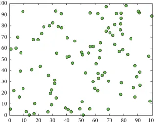
Figure 2: The randomly deployed sensor nodes in a WSN.
10 0 20 30 40 50 60 70 80 90 100 0 10 20 30 40 50 60 70 80 90 100
Figure 3: The cluster formation and CHs after the set-up phase.
The TDMA schedule allocates specific time intervals for each of the cluster members to transmit their collected data to their CHs in LEFCA. TDMA schedule not only prevents the collisions among data messages but also enables the radio components of each regular node to put to sleep mode at all times except during their transmit time, thus providing energy savings.
After the reception of the TDMA schedule by the cluster member nodes, the set-up phase is completed and data transmission with steady-state phase is ready to start. Figure 2 shows an example of randomly deployed sensor nodes in a WSN and Figure 3 shows an example illustration of the clusters formed after the LEFCA set-up phase.
3.2. Steady-State Phase. The main objective of the steady-state phase is to transmit the collected data to the base station through the CHs and to determine whether a CH change needs to be made. Figure 4 shows a typical round for the LEFCA algorithm with its two subphases: data transmission and CH change decision.
3.2.1. Data Transmission Phase. This phase is divided into slots allocated for each of the cluster members, where the member nodes transmit their data to the CH. The duration for each slot is fixed; thus the time to transmit data hinges on the number of member nodes in the cluster. When the data collection from the cluster members is complete, the CH transmits collected data to the base station.
Transmission in one cluster can affect communication in a nearby cluster. To reduce intercluster interference, each cluster in LEFCA communicates by the help of these unique spreading codes. Within a cluster, every node uses a common transmitting code so that there is no intercluster collision in transmitter-based code assignment mechanism. If two nodes in a cluster are not transmitting simultaneously, there will be also no intracluster collision. From the predefined list, the CHs obtain these codes according to their advertisement order and they use these codes within their clusters. When transmitted data from associated members are reached to the CH, CH filters all received energy using this spreading code. Combining DS-SS with a TDMA schedule in LEFCA decreases intercluster interference while eliminating intra-cluster interference.
Note that CH transmits the collected data from its associated members using a fixed spreading code and a CSMA structure. CH listens to the channel to hear if anyone else is sending data to the BS using the BS spreading code, if not CH transmits the data to the BS using the BS spreading code. Otherwise, CH waits to send the data to the BS. 3.2.2. CH Change Decision Phase. The LEFCA algorithm uses fixed clusters; thus a sensor node which becomes a member of a cluster during the set-up phase stays as a member of the same cluster for the entire lifetime of the sensor network. However, the CHs may change at the beginning of a new LEFCA round.
When data transmission phase of a round is complete, the CH needs to decide whether it will continue to act as a CH for the next round or choose a new CH. This decision is made based on the CH’s remaining energy. If the CH’s remaining energy is above a predefined threshold value (ThV), it continues to act as the CH for the next round and notifies the cluster members by specifying its CH ID. If on the other hand the CH’s remaining energy is below the ThV, the current CH selects a new cluster head which will become the new CH in the next round and notifies the cluster members by specifying the new CH’s ID. If a new CH needs to be elected the current CH chooses the new one randomly among the alive members of its cluster. Figure 5 illustrates the CH change mechanism in LEFCA while keeping the clusters fixed.
Determination of (ThV) is an important step for LEFCA because the ThV has a significant impact on the network lifetime. If the ThV is very small, the CH might die during a round resulting in network disconnectivity. If the ThV is large, the algorithm might select a new CH for every round resulting in larger network and set-up costs. ThV is selected to be equal to initial energy of a node, the CHs will change, at every round, and LEFCA will behave like the LEACH protocol.
Slot for Slot for node 2
LEFCA round
Data transmission phase
CH change decision phase CH ID Sent data to BS Time Slot for node 3 Slot for node 4 Slot for node 1 · · · node k
Figure 4: The LEFCA round. Data transfers and changing of CHs if needed occur during the steady-state phase.
10 0 20 30 40 50 60 70 80 90 100 0 10 20 30 40 50 60 70 80 90 100
Figure 5: CH changes in LEFCA.
To reduce the networking and clustering costs seen with traditional LEACH, the ThV should be determined in such a way that the CH should be alive at the end of the round to keep network connectivity. Equation (1) can be used to determine the minimum ThV which assures certain network connectivity. The energy dissipated in the CH node during a single frame is
𝐸CH= 𝑙𝐸elec(𝑁𝑘 − 1) + 𝑙𝐸DA(𝑁𝑘) + 𝑙𝐸elec + 𝑙𝜀mp𝑑4toBS,
(1)
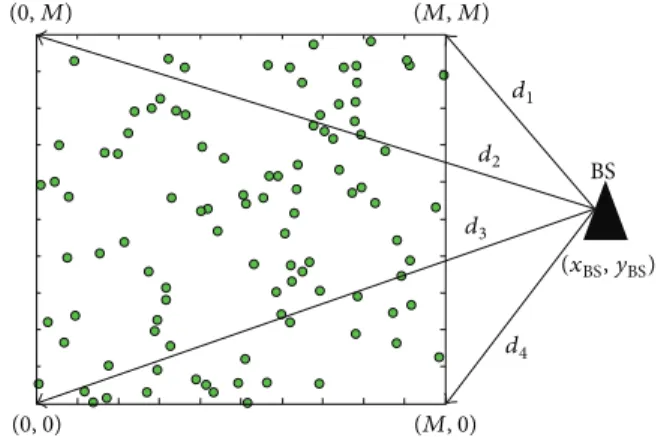
where𝑙 is the length of the transmitted bits by each cluster member,𝐸elecis the transceiver energy,𝐸DAis the aggregation energy per bit,𝑁/𝑘 is the average number of nodes in clusters, 𝜀mp is multipath amplifier energy with 𝑑4 power loss, and 𝑑toBSis the distance of the CH to the BS. To determine the ThV which assures certain network connectivity the farthest node to the BS should be considered. Assume that the farthest node to the BS has the coordinates of(𝑥, 𝑦) and, for instance, the BS is located at outside of the sensor field as(𝑥BS, 𝑦BS) which is shown in Figure 6. To find the energy consumption of the farthest CH node in the network, (1) can be used but first of all𝑑4toBS value should be calculated. The maximum value of distance to the BS which minimizes the ThV can be obtained by using following figure and equations. Let us assume that sensor nodes are deployed randomly in a square
(0, 0) (0, M) (M, M) (M, 0) d1 d2 d3 d4 BS BS) y (xBS,
Figure 6: Outside BS situation.
field which has𝑀 × 𝑀 m2area. To find the farthest node to the BS the maximum values of𝑑1to𝑑4should be calculated:
𝑑1= max (√(𝑥BS− 𝑀)2+ (𝑦BS− 𝑀)2) 𝑑2= max (√(𝑥BS)2+ (𝑦BS− 𝑀)2) 𝑑3= max (√(𝑥BS)2+ (𝑦BS)2) 𝑑4= max (√(𝑥BS− 𝑀)2+ (𝑦BS)2) (2) 𝑑toBS= max (𝑑1, 𝑑2, 𝑑3, 𝑑4) . (3) The value of𝑑toBSin (3) will give us the distance of the farthest node to the BS.
For example, assume that the farthest node to the BS has the coordinates of(0, 0) and the BS is located at outside of the sensor field at(150, 50). To find the energy consumption of the farthest CH node in the network, (1) can be used. From (3),𝑑toBSis calculated as
𝑑toBS= √(150 − 𝑥)2+ (50 − 𝑦)2
𝑑toBS= √(150 − 0)2+ (50 − 0)2= 158.1139. (4)
To determine the ThV, it is assumed that only one cluster is formed and the(𝑥, 𝑦) coordinates of the CH are (0, 0) (the worst scenario). Thus,𝑘 = 1 (only one cluster is formed); hence,𝑁/𝑘 = 100.
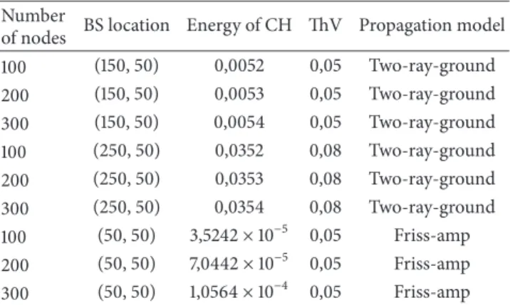
Table 1: Determination of ThV. Number
of nodes BS location Energy of CH ThV Propagation model 100 (150, 50) 0,0052 0,05 Two-ray-ground 200 (150, 50) 0,0053 0,05 Two-ray-ground 300 (150, 50) 0,0054 0,05 Two-ray-ground 100 (250, 50) 0,0352 0,08 Two-ray-ground 200 (250, 50) 0,0353 0,08 Two-ray-ground 300 (250, 50) 0,0354 0,08 Two-ray-ground 100 (50, 50) 3,5242× 10⁻⁵ 0,05 Friss-amp 200 (50, 50) 7,0442× 10⁻⁵ 0,05 Friss-amp 300 (50, 50) 1,0564× 10⁻⁴ 0,05 Friss-amp
For experiments in LEFCA, 𝑙 = 6400 bits, 𝐸elec = 50 nJ/bit, 𝑁/𝑘 = 100, 𝐸DA = 5 nJ/bit, 𝜀mp = 0.0013 pJ, and finally𝑑4toBS= 6.25 × 10⁸m4.
When these values are placed into (1),
𝐸CH∼ 0.0052. (5)
According to result in (5), if remaining energy of any CH node in the system is greater than 0.0052 it can survive certainly for a round. Thus, to provide connectivity between any CH with BS, the ThV should be chosen greater than this value; thus it is determined as 0.05 J. Table 1 shows the ThVs for various networks with different number of nodes, BS locations.
Note that, in a typical round, a CH node will consume significantly more energy than the regular nodes and the basic motivation behind LEFCA algorithm is to abuse the CH node by keeping it as a CH as much as possible while trying to keep the regular nodes’ energy at a maximum. This type of CH changing mechanism provides substantial energy savings, as new cluster topologies are not formed for every round. There is no need to use advertisement, join request, and TDMA schedule messages for each round as the clusters are fixed.
4. Simulation and Performance
Analysis of LEFCA
In order to measure the performance of LEFCA, an extensive set of simulations are conducted in an area of 100 × 100 meters with 100 randomly deployed sensors. The base station is located outside the sensor field at coordinates (150, 50). Each simulation is repeated 100 times with different sensor deployments and unless otherwise stated the average perfor-mance measures are presented.
A simple model for the radio hardware energy con-sumption is used to run the simulations. The transmitting nodes dissipate energy to run the radio electronics and the power amplifier. The receiving nodes consume energy to run the radio electronics. Depending on the distance between a transmitter and a receiver, cross-over distance𝑑co, fs (free space with𝑑2power loss), or mp (multipath fading with𝑑4 power loss) channel models are used [10].
Table 2: Simulation environment parameters.
Parameters Values
Network area 100 m× 100 m
Number of nodes 100
Base station coordinates (150, 50) Initial energy per node 2 J Data packet size 6400 bits Control packet size 200 bits Transceiver energy 50 nJ/bit Aggregation energy per bit 5 nJ/bit/signal Free space amplifier energy 10 pJ/bit/m2 Multipath amplifier energy 0.0013 pJ/bit/m4
Thus, to transmit𝑙-bit message through a distance 𝑑 the radio expends 𝐸TX(𝑙, 𝑑) = { { { 𝑙𝐸elec+ 𝑙𝜀fs𝑑2, 𝑑 < 𝑑 co 𝑙𝐸elec+ 𝑙𝜀mp𝑑4, 𝑑 ≥ 𝑑 co (6)
and to receive a message, radio expends
𝐸RX(𝑙) = 𝑙𝐸elec. (7)
The transceiver energy(𝐸elec) depends on digital coding, modulation, spreading of the signal, and filtering. The free space amplifier energy (𝜀fs) and the multipath amplifier energy(𝜀mp) depend on the distance to the receiver and the acceptable bit-error rate. Table 2 summarizes the simulation environment parameters used for simulations.
In the simulations, the impact of the random and intel-ligent CH selection mechanisms and the ThV on the perfor-mance of LEFCA is observed. The energy map of the network is studied for a sample topology to understand how the CH abusement effects the energy distribution in the network. To compare LEFCA’s performance with other important algorithms, LEACH and its two successful variants (LEACH-F and ModLEACH) are chosen. In addition to LEACH variants, LEFCA is compared with two novel heterogenous algorithms SEP and DEEC. The comparisons are made in terms of residual energy, number of alive nodes, and network lifetime.
4.1. Cluster Topologies with Intelligent CH Selection. Since the clusters will remain fixed throughout the entire WSN lifetime, the initial cluster topologies are very important. Figures 7, 8, 9, and 10 show the cluster topologies based on intelligent CH selection mechanism of LEFCA for 5, 6, 9, and 10 clusters, respectively. Depending on the desired number of clusters LEFCA selects the sensor nodes which are closest to the center of each cluster as the CHs. For example, if the desired number of clusters is 6, the network is divided into 6 pieces and the nodes at the center (or closest to the center) of each piece become the CHs. The remaining nodes join to a CH which is nearest to their positions and the cluster topologies are formed.
10 0 20 30 40 50 60 70 80 90 100 0 10 20 30 40 50 60 70 80 90 100
Figure 7: WSN for 5 clusters.
10 0 20 30 40 50 60 70 80 90 100 0 10 20 30 40 50 60 70 80 90 100
Figure 8: WSN for 6 clusters.
4.2. Comparison of Random and Intelligent CH Selection Mechanisms of LEFCA. In this part, LEFCA is analyzed for its lifetime when CHs are selected based on the intelligent CH selection mechanism or randomly. For each value of the number of clusters, the average and 95% confidence interval values of lifetime are obtained for 100 iterations of a sensor network with 100 nodes.
As can be seen from Figure 11, the average lifetime of the WSN increases significantly with the intelligent CH selection. The difference increases as the number of clusters increases. For example, for a network with 10 clusters, the lifetime gain is approximately 800 rounds. Thus, intelligent CH selection outperforms traditional random CH selection method for lifetime and energy-efficiency.
4.3. Impact of ThV in Network Lifetime. Figure 12 compares the performance of LEACH and LEFCA for different ThVs by illustrating the number of dead nodes versus round number. From this figure, it can be observed that as the ThV increases the network lifetime decreases. A lower ThV also results in an earlier first node death as LEFCA abuses the CHs before
10 0 20 30 40 50 60 70 80 90 100 0 10 20 30 40 50 60 70 80 90 100
Figure 9: WSN for 9 clusters.
10 0 20 30 40 50 60 70 80 90 100 0 10 20 30 40 50 60 70 80 90 100
Figure 10: WSN for 10 clusters.
Rand selection average Intel-selection average Rand selection con-int-low
Rand selection con-int-high
Intel-selection con-int-low Intel-selection con-int-high 4 5 6 7 8 9 10 11 12 13 14 Number of clusters 3600 3800 4000 4200 4400 4600 4800 5000 5200 5400 5600 Li fe ti m e
Figure 11: Comparison lifetime performance of random and intel-ligent CH selection of LEFCA in terms of number of clusters.
LEACH ThV = 0.4 ThV = 0.5 ThV = 0.15 ThV = 0 ThV = 0.25 1000 2000 3000 4000 5000 6000 0 Round number 0 10 20 30 40 50 60 70 80 90 100 N u m b er o f de ad no des
Figure 12: Number of dead nodes according to the different ThVs.
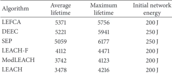
Table 3: Network lifetime comparison. Algorithm Average lifetime Maximum lifetime Initial network energy LEFCA 5371 5756 200 J DEEC 5221 5941 250 J SEP 5059 6177 250 J LEACH-F 4112 4471 200 J ModLEACH 3742 4123 200 J LEACH 3478 4216 200 J
selecting a new CH. However, the lifetime gain for any ThV is very significant.
Note that the lifetime of LEACH for the same network is approximately 3200 rounds and a significant improvement for network lifetime is achieved with LEFCA.
4.4. Energy Map of the Network. The energy consumption for the individual nodes under LEFCA and LEACH protocols is analyzed through simulation studies in order to understand the energy dissipation of the entire network. The average lifetime of the LEACH protocol is approximately 3500 rounds for a network consisting of 100 nodes which is obtained from simulations as shown in Table 3.
Figure 13 shows the energy map of the LEACH protocol at round number 3500. At this round, approximately half of the nodes are dead and very few nodes closer to the BS have a very small amount of remaining energy in the order of0.1𝐸0. In LEACH, the alive nodes will quickly drain their remaining energy and the network will lose its complete functionality. On the other hand, Figure 14 shows the energy map of the LEFCA protocol at round number 3500, when LEACH is almost dead. Compared to LEACH, two-thirds of the nodes are still alive with significantly higher energy levels. The alive nodes still have0.5𝐸0of their total initial energy; thus, the
CH CH CH CH 0 10 20 30 40 50 60 70 80 90 100 10 0 20 30 40 50 60 70 80 90 100 E < 0.9E0 E < 0.8E0 E < 0.7E0 E < 0.6E0 E < 0.5E0 E < 0.4E0 E < 0.3E0 E < 0.2E0 E < 0.1E0 E = 0
Figure 13: Energy map of LEACH at round 3500.
CH CH CH CH CH CH CH CH CH CH 0 10 20 30 40 50 60 70 80 90 100 10 0 20 30 40 50 60 70 80 90 100 E < 0.9E0 E < 0.8E0 E < 0.7E0 E < 0.6E0 E < 0.5E0 E < 0.4E0 E < 0.3E0 E < 0.2E0 E < 0.1E0 E = 0
Figure 14: Energy map of LEFCA at round 3500.
LEFCA protocol will be able to collect data from each of the clusters at the upcoming rounds.
Figure 15 shows the energy map of LEFCA at round 4600. While the network is completely dead for the LEACH protocol at this round, LEFCA can still gather data from WSN. Contrary to LEACH protocol at round 3500, the alive nodes are distributed across the entire network, giving a possibility to reach even the furthest clusters. By design, the LEACH protocol forms clusters for every round which brings excessive network costs, overhead, and energy consumption.
CH CH CH CH CH CH CH CH CH E < 0.9E0 E < 0.8E0 E < 0.7E0 E < 0.6E0 E < 0.5E0 E < 0.4E0 E < 0.3E0 E < 0.2E0 E < 0.1E0 E = 0 0 10 20 30 40 50 60 70 80 90 100 10 0 20 30 40 50 60 70 80 90 100
Figure 15: Energy map of LEFCA at round 4600.
With LEACH, the nodes which are farthest to the BS die first and hence equal load and energy distribution cannot be obtained once there are dead nodes in the network. Collecting information from remote clusters of the WSN becomes increasingly impossible as the network grows old. On the other hand, LEFCA tries to maintain full network connectivity when compared with LEACH. LEFCA abuses the energy of the CHs until their residual energy falls down the ThV. When a new CH change is needed, the CH is randomly chosen from the members of the same cluster. The CH change mechanism of LEFCA also decreases the number of CH changes in WSN. With less number of CH changes, the additional network traffic and overhead are reduced and energy-efficiency can be maintained. Because of these reasons, LEFCA not only improves the network lifetime but also makes it possible to collect data from the entire network topology at all times.
4.5. Residual Energy. The energy consumption rate in a WSN can vary significantly with the employed routing algorithm and directly impacts the lifetime of the WSN. Figure 16 compares the total residual energy of LEFCA with LEACH, LEACH-F, ModLEACH, DEEC, and SEP. While LEFCA, LEACH, LEACH-F, and ModLEACH use homogeneous net-works where all the nodes are identical with the same initial energy, SEP and DEEC use heterogeneous networks where some of the nodes have more initial energy compared to the rest of the nodes. Thus, the total initial energy of the WSN with SEP and DEEC is 250 J while for the other algorithms it is 200 J.
It is observed that the energy consumption rate of LEFCA is the lowest among all compared algorithms. The fixed clustering approach complemented with full utilization of the CHs results in fewer number of CH changes and provides a
LEACH-F LEACH ModLEACH LEFCA DEEC SEP 1000 2000 3000 4000 5000 6000 0 Round number 0 50 100 150 200 250 Resid ual ener g y
Figure 16: Round number versus residual energy.
conservative energy consumption for LEFCA. For example, after 2000 rounds LEACH holds 15% of its initial total energy, while LEFCA holds approximately 50% of its initial total energy. When the entire energy of the network is spent under LEACH, LEFCA still maintains 20% of its total initial energy. Although SEP and DEEC start with 25% more initial energy, LEFCA’s conservative energy consumption yields in a better residual energy after round 800 for DEEC and round 1950 for SEP. Thus, LEFCA is an energy-efficient algorithm.
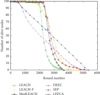
4.6. Number of Alive Nodes. Clustering is a fundamental way for extending the lifetime of a WSN. In Figure 17, various cluster based routing algorithms are compared based on the number of alive nodes. The lifetimes are measured when all the algorithms start with an initial number of 100 alive nodes. When compared with LEACH, a 57% improvement in the network lifetime can be observed under LEFCA. While LEACH lasts for 3237 rounds, LEFCA lasts for 5659 rounds. Not only does LEFCA have a longer lifetime than LEACH and its variants (LEACH-F and ModLEACH) but also a comparison with SEP and DEEC (both have 25% more initial network energy) yields a longer lifetime for LEFCA. Node deaths start earlier under LEFCA, but the rate of node deaths is much lower than all the algorithms compared. While trying to transmit the collected information through abused CHs, infrequent CH changes keep remaining nodes’ energy levels as high as possible under LEFCA and node deaths are distributed almost evenly for the network lifetime. For LEACH based protocols and SEP, following the first node death, the remaining node deaths occur quickly. As a consequence, a longer lifetime is achieved under LEFCA. 4.7. Network Lifetime. For each algorithm, the simulations are repeated 100 times for different topologies and the maximum and average observed lifetimes are presented in Table 3 as
LEACH-F LEACH ModLEACH LEFCA DEEC SEP 0 10 20 30 40 50 60 70 80 90 100 N um b er o f ali ve no des 1000 2000 3000 4000 5000 6000 0 Round number
Figure 17: Round number versus number of alive nodes.
well as the initial network energies. LEFCA’s conservative energy consumption ratio increases the lifetime of a WSN significantly. LEFCA outperforms LEACH and its variants. When LEFCA is compared with novel routing algorithms such as SEP and DEEC, extended lifetimes are also observed although LEFCA starts with lower initial energy.
5. Conclusions and Future Work
In this paper, a fixed clustering based routing protocol (LEFCA) for WSNs is proposed. In the past decade, the exponential growth of the ICT led to research for green networking to provide energy-efficient solutions at all layers of the Internet protocol stack. For WSNs, an energy-efficient routing protocol can increase the lifetime of the network. LEFCA achieves this objective through fixed number of clusters and reduced number of CH changes. For the LEACH algorithm and most of its variants, the clusters and CHs change at every round resulting in an excessive amount of energy consumption. On the other hand, LEFCA keeps the same cluster topology formed at the start of the network for the entire lifetime and minimizes CH changes with a threshold based CH change mechanism. By this way, LEFCA spends the network energy in a conservative manner and increases the network lifetime. When the performance of LEFCA is compared with traditional and novel routing algorithms, significant gains are observed in terms of energy usage and lifetime.
Due to the distance factor, the clusters that are farthest from the base station tend to consume more energy under LEFCA. The first nodes that die in the network are usually the members of far clusters. Further improvement in the performance of LEFCA can be obtained by placing relay nodes and transmitting the collected data through the relay nodes in a multihop communication method. By this way, the lifetime of far nodes can be extended.
Under LEFCA, the initial CHs are selected in an intel-ligent way to form the clusters. However, the subsequent CH changes are made randomly. Instead of picking up a random cluster member to become the next CH, the nearest member or the member with the maximum remaining energy can be chosen. This approach also has a further potential improvement for the performance of LEFCA.
Competing Interests
The authors declare that they have no competing interests.
References
[1] T. Rault, A. Bouabdallah, and Y. Challal, “Energy efficiency in wireless sensor networks: a top-down survey,” Computer
Networks, vol. 67, pp. 104–122, 2014.
[2] A. M. S. Saleh, B. M. Ali, M. F. A. Rasid, and A. Ismail, “A survey on energy awareness mechanisms in routing protocols for wireless sensor networks using optimization methods,”
Transactions on Emerging Telecommunications Technologies, vol.
25, no. 12, pp. 1184–1207, 2014.
[3] T. Da˘g and K. Cengiz, “Towards energy-efficient MAC pro-tocols,” in Proceedings of the 18th World Multi-Conference on
Systemics, Cybernetics and Informatics (WMSCI ’14), pp. 86–90,
Orlando, Fla, USA, July 2014.
[4] V. Mor and H. Kumar, “Energy efficient wireless mobile net-works: a review,” in Proceedings of the International
Confer-ence on Reliability, Optimization and Information Technology (ICROIT ’14), pp. 281–285, Haryana, India, February 2014.
[5] K. Cengiz and T. Da˘g, “A review on the recent energy-efficient approaches for the Internet protocol stack,” EURASIP Journal
on Wireless Communications and Networking, vol. 2015, article
108, 2015.
[6] C. Zhu, L. Shu, T. Hara, L. Wang, S. Nishio, and L. T. Yang, “A survey on communication and data management issues in mobile sensor networks,” Wireless Communications and Mobile
Computing, vol. 14, no. 1, pp. 19–36, 2014.
[7] D. Singh, G. Tripathi, and A. J. Jara, “A survey of internet-of-things: future vision, architecture, challenges and services,” in
Proceedings of the IEEE World Forum on Internet of Things (WF-IoT ’14), pp. 287–292, Seoul, South Korea, March 2014.
[8] P. Ostovari, J. Wu, and A. Khreishah, “Network coding tech-niques for wireless and sensor networks,” in The Art of Wireless
Sensor Networks, Signals and Communication Technology, pp.
129–162, Springer, Berlin, Germany, 1st edition, 2014.
[9] W. Heinzelman, C. Anantha, and B. Hari, “Energy-efficient communication protocol for wireless microsensor networks,” in Proceedings of the 33rd IEEE Annual Hawaii International
Conference on System Sciences, pp. 1–10, Maui, Hawaii, USA,
January, 2000.
[10] W. B. Heinzelman, A. P. Chandrakasan, and H. Balakrish-nan, “An application-specific protocol architecture for wireless microsensor networks,” IEEE Transactions on Wireless
Commu-nications, vol. 1, no. 4, pp. 660–670, 2002.
[11] S. Soro and W. B. Heinzelman, “Prolonging the lifetime of wireless sensor networks via unequal clustering,” in Proceedings
of the 19th IEEE International Parallel and Distributed Processing Symposium (IPDPS ’05), pp. 1–8, Denver, Colo, USA, April 2005.
[12] L. Zhao and Q. Liang, “Distributed and energy efficient self-organization for on-off wireless sensor networks,” in Proceedings
of the IEEE 15th International Symposium on Personal, Indoor and Mobile Radio Communications (PIMRC ’04), pp. 211–215,
Barcelona, Spain, September 2004.
[13] H. Junping, J. Yuhui, and D. Liang, “A time-based cluster-head selection algorithm for LEACH,” in Proceedings of the 13th IEEE
Symposium on Computers and Communications (ISCC ’08), pp.
1172–1176, Marrakech, Morocco, July 2008.
[14] M. S. Ali, T. Dey, and R. Biswas, “ALEACH: advanced LEACH routing protocol for wireless microsensor networks,” in Proceedings of the 5th International Conference on Electrical
and Computer Engineering (ICECE ’08), pp. 909–914, Dhaka,
Bangladesh, December 2008.
[15] W. N. W. Muhamad, K. Dimyati, R. Mohamad et al., “Evaluation of stable cluster head election (SCHE) routing protocol for wire-less sensor networks,” in Proceedings of the IEEE International
RF and Microwave Conference (RFM ’08), pp. 101–105, Kuala
Lumpur, Malaysia, December 2008.
[16] M. M. Shirmohammadi, K. Faez, and M. Chhardoli, “LELE: leader election with load balancing energy in wireless sensor network,” in Proceedings of the WRI International Conference
on Communications and Mobile Computing (CMC ’09), pp. 106–
110, IEEE, Beijing, China, January 2009.
[17] F. Ayughi, K. Faez, and Z. Eskandari, “A non location aware version of modified LEACH algorithm based on Residual Energy and Number of Neighbors,” in Proceedings of the 12th
International Conference on Advanced Communication Tech-nology: ICT for Green Growth and Sustainable Development (ICACT ’10), pp. 1076–1080, Gangwon-Do, Republic of Korea,
February 2010.
[18] Z.-G. Sun, Z.-W. Zheng, and S.-J. Xu, “An efficient routing pro-tocol based on two step cluster head selection for wireless sensor networks,” in Proceedings of the 5th International Conference on
Wireless Communications, Networking and Mobile Computing (WiCOM ’09), pp. 1–9, Beijing, China, September 2009.
[19] X. Hu, J. Luo, Z. Xia, and M. Hu, “Adaptive algorithm of cluster head in wireless sensor network based on LEACH,” in Proceedings of the IEEE 3rd International Conference on
Communication Software and Networks (ICCSN ’11), pp. 14–18,
Xi’an, China, May 2011.
[20] A. Azim and M. M. Islam, “A dynamic round-time based fixed low energy adaptive clustering hierarchy for wireless sensor networks,” in Proceedings of the IEEE 9th Malaysia International
Conference on Communications with a Special Workshop on Digital TV Contents (MICC ’09), pp. 922–926, Kuala Lumpur,
Malaysia, December 2009.
[21] D. Mahmood, N. Javaid, S. Mahmood, S. Qureshi, A. M. Memon, and T. Zaman, “MODLEACH: a variant of LEACH for WSNs,” in Proceedings of the IEEE 8th International Conference
on Broadband, Wireless Computing, Communication and Appli-cations (BWCCA ’13), pp. 158–163, Compeigne, France, October
2013.
[22] G. Smaragdakis, I. Matta, and A. Bestavros, “SEP: a stable election protocol for clustered heterogeneous wireless sensor networks,” in Proceedings of the 2nd International Workshop on
Sensor and Actor Network Protocols and Applications (SANPA ’04), Boston, Mass, USA, 2004.
[23] L. Qing, Q. Zhu, and M. Wang, “Design of a distributed energy-efficient clustering algorithm for heterogeneous wireless sensor networks,” Computer Communications, vol. 29, no. 12, pp. 2230– 2237, 2006.
[24] K. Pahlavan and A. Levesque, Wireless Information Networks, John Wiley & Sons, New York, NY, USA, 1995.