African Journal of Business Management Vol. 5(16), pp. 7017-7030, 18 August, 2011 Available online at http://www.academicjournals.org/AJBM
DOI: 10.5897/AJBM11.672
ISSN 1993-8233 ©2011 Academic Journals
Full Length Research Paper
The behaviour of the Istanbul stock exchange market:
An intraday volatility/return analysis approach
Veysel Ulusoy
1, M. Hasan Eken
2and Serkan Çankaya
3*
1Faculty of Economics and Administrative Sciences, Istanbul Aydın University, Turkey. 2Institute of Social Sciences, Kadir Has University, Turkey.
3
Faculty of Economics and Administrative Sciences, Beykent University, Turkey Accepted 17 May, 2011
This study investigates intraday effects in the Istanbul Stock Exchange (ISE) during the latest period of financial turmoil which began in August 2007 and extended to February 2010. We tested for the possible existence of intraday anomalies using both return and volatility equations, empirically applying GARCH (p,q) models. The unique data set we utilized was compiled from 15-min intraday values of the ISE-100 Index which are formed by averaging historical ten-second tick data. This study contributes to the current literature in three distinct ways. Firstly, the basic characteristics of the unique data used in this research were investigated in detail. Secondly, four range-based volatility measures, namely Garman Klass (GK), Yang-Zhang (YZ), Rogers-Satchell (RS) and Parkinson (PK), were employed to take more precise measurements of volatility for intraday data analysis in order to identify the changes in general market sentiment using opening, closing, high and low prices. Thirdly, we estimated the relative efficiency of GK, YZ, RS and PK by applying GARCH (p,q) models. The results are quite promising, indicating that strong opening price jumps are present for daily and morning calculations. They illustrate that the YZ estimator has relatively more power in generating tolerable volatility patterns. Key words: Intraday volatility, GARCH, Istanbul Stock Exchange.
INTRODUCTION
Estimating the volatilities of equity prices from historical data has received considerable attention, both from academicians and market professionals. Many empirical tests have been conducted to examine the efficiency of stock markets around the world, using stock prices, transaction data, volatility and the intraday frequency of bid and ask spreads. Wood et al. (1985) found a number of patterns in trading frequency such as number of shares per trade, size of price changes, length of time between trades and the absolute values of price changes. They used minute-by-minute market return changes to test normality and autocorrelation and showed that unusually high returns and standard deviations were
*Corresponding author. E-mail: [email protected]. Tel: 90 212 867 51 40
found at the beginning and at the end of the day. Similar results were found by Harris (1986) using intraday returns over 15-min intervals. He showed that there was a significant difference in intraday returns during the first 45 min after the opening of markets. Smirlock and Starks (1986) studied the Dow Jones Industrial Average stock returns on an hourly basis data and they observed that on average Monday mornings provide negative returns.
Further evidence of the differences across trading hour returns were further examined by Jain and Joh (1988). They extended previous studies by including the average daily trading volume for each trading hour. It was found that the average daily trading volume was lowest on Monday, increased until Thursday and declined again on Thursday and Friday. Their results suggest that the average trading volume across the six daily trading hours differs considerably. The first hour has the highest average volume which then declines until the fourth hour
and then increases in the fifth and sixth hours.
Harris (1989) extended his previous research and examined transaction prices to further characterize the systematic day-end price rise. He drew attention to the importance of the first and last few transactions. McInish and Wood (1990a) confirmed their earlier study through the use of New York Stock Exchange data from 1980 to 1984. They found a high level of variance of returns at the beginning and at the end of the trading day. Evidence of a U-shaped pattern in the variance of price changes according to the hour of the day was also reported by Foster and Viswanathan (1990) and Gerety and Mulherin (1992).
Lockwood and Linn (1990) extended previous volatility studies by examining the market variance of returns on the Dow Jones Industrial Average for the period 1964 to 1989. According to their study, return volatility decreases from the opening hour until early afternoon and then subsequently increases, and is considerably greater for intraday versus overnight periods.
The availability of transaction data in the mid-1980s for U.S. exchanges boosted the amount of empirical research that could be done in this specific field. Similar research results were observed in other markets during those years as well. Increasing availability of non-U.S. equity market intraday transactions data during the 1990s has encouraged the extension of international studies in other national stock exchanges. McInish and Wood (1990b) found that the stocks on the Toronto Stock Exchange showed a U-shaped return and volume pattern. Similar results have been reported for the Stockholm Stock Exchange (Niemayer and P. Sandas 1993), the Australian SEATS trading system (Aitken et al., 1993), the London Stock Exchange (Yadav and Pope, 1992), the Tokyo Stock Exchange (Chang et al., 1993), and the German Stock Exchange (Lowengrub and Melvin, 2002).
According to the results of these empirical studies, there is systematic inefficiency and variation in stock prices as related to the calendar year. However, another stream of research claims that these patterns are a product of the market structure. Stoll and Whaley (1990) attributed greater volatility in the NYSE to private information revealed in trading and to temporary price deviations induced by specialists and other traders. Hong and Wang (2000) demonstrated that market closures in the U.S. market can affect investors’ trading policies and the resulting return generating process. There is evidence of this from other markets as well. Cyree and Winters (2001) studied the federal funds market in the U.S. and found that the reverse-J pattern in intraday returns, variances and volume can be explained by trading stops, and they proposed that private information is not a necessary condition for the pattern that has been observed. However, the authors also point out that, according to their results, “private information does not play a role in intraday patterns in other securities markets but rather, that private information is not a necessary condition for the observed intraday pattern.” Another
study by Akay et al. (2010) about the federal funds market which examines the efficiency of several range-based volatility estimators showed that range-range-based estimators remove the upward bias created by micro-structure noise.1 Ederington and Lee (1993) examined the impact of scheduled macroeconomic news announce-ments on interest rates and foreign exchange futures markets and found that the observed intraday and day of the week volatility patterns in these markets are mainly due to the timing of major macroeconomic announce-ments. The authors also noted that when the impacts of these announcements are removed, volatility is basically flat across the trading day and the trading week. Kalev and Pham (2009) examined the impact of the time of day and day of the week on patterns of trading by informed investors. They found an inverted U-shaped pattern of investors’ intraday trading activities and suggested that informed traders select an optimum day of the week to trade that will minimize their transaction costs. They also demonstrate that informed traders use different trading strategies depending on the time of day.
There is still an ongoing debate about the findings of the studies afore mentioned. Some consider them to be the fruit of data mining whereas others defend the findings of previous research and seek to find rational explanations for any irrational results. As a result of these studies, however, there has emerged a phenomena referred to as calendar anomalies. Studies of calendar anomalies have shown that asset returns vary on different days of the week, times of the month and months of the year, as well as before holidays, and even in intraday patterns. These effects have been taken as evidence usable against the efficient market hypothesis.
As regards the related literature about the Turkish Stock Exchange, the only detailed research specifically aimed at intraday patterns was conducted by Bildik (2001). His findings were also consistent with the results of previous research in other international studies, and Bildik (2001) showed that intraday effects also existed in the Istanbul Stock Exchange Market. He used 15-min (as well as 5- and 1-min) interval data for the years between 1996 and 1999. He also found that opening and closing returns were large and positive, and that volatility was higher at opening times and followed an L-shaped pattern. He concluded that the relatively higher mean and standard deviation in opening sessions was generated by an accumulation of overnight information and the closed-market effect (halt of trade). The large day-end returns were affected by the activities of fund managers and speculators for the window-dressing around close time.
This study focuses on analyzing the market behavior of the Istanbul Stock Exchange (ISE) during the latest period of financial turmoil which extended from August
1 Akay et.al define “microstructure noise” as follows: A time series of security prices has volatility that decomposes into economic volatility and trading process volatility. Trading process volatility is induced by the mechanics of trading and arises from the use of transaction level data.
2007 to February 2010. We test for the possible existence of intraday anomalies by using both return and volatility equations, empirically applying GARCH (p,q) models. This study utilizes a unique data set which was compiled from 15-min intraday values of the ISE-100 Index which are formed by averaging historical ten second tick data.
This study contributes to the current literature in three distinct ways. Firstly, the basic characteristics of the unique data used in this research were investigated in detail. Secondly, four range-based volatility measures, namely GK, YZ, RS and PK, were employed to take more precise measurements of volatility for intraday data analysis in order to identify the changes in general market sentiment using opening, closing, high and low prices. Thirdly, we estimated the relative efficiency of GK, YZ, RS and PK by applying GARCH (p,q) models, although there are other studies that have sought to examine different calendar anomalies (Demirer and Baha, 2002; Aydoğan and Booth, 2003;Bildik, 2004). The exis-ting research about the intraday effect as a behavioral pattern of the Istanbul Stock Exchange is very limited.
This study differs from previous research in that it ex-plicitly analyzes the intraday effects of the trading hours in Turkey with a focus on the period of financial instability from 2007 to 2010. Another distinction is that this study analyzes the trading day for three different periods; daily, morning and afternoon sessions were investigated se-parately and then compared to reveal any discrepancies.
INSTITUTIONAL BACKGROUND OF THE ISTANBUL STOCK EXCHANGE
The Istanbul Stock Exchange (ISE) is a relatively young stock exchange market in comparison to the stock ex-changes of developed countries. The ISE was founded in 1986, and as of February 1, 2010, there were 316 listed stocks. Total market capitalization is approximately U.S. $ 316 billion, and as of 2009, the average daily volume was around U.S. $ 1.25 billion.
There have been major developments at the ISE over the last couple of years. One such development is that, on June 1, 2009, the ISE introduced an Automated Dis-closure Platform, which is an electronic system, enabling companies traded on the ISE to release any information which must be publicly disclosed in compliance with respective legislation. This technology was made possible with the use of Internet and electronic signature technologies.
Another development at the ISE is the concept of making. It has been decided that the market-making process shall be executed via a method referred to as the “continuous auction trading method,” and this is to be applied in the absence of a market maker. These market making operation principles were determined at the meeting of the Executive Council of the Exchange on February 4, 2009.
Ulusoy et al. 7019
Trades are executed automatically in the ISE per the multiple price-continuous auction principle based on price and time priority rules via an electronic trading system. Trades are executed in two trading sessions, morning and afternoon. An opening session based on the single price system is organized at the beginning of the morning session.
Another change at the ISE concerns trading hours. Effective October 13, 2008, trading hours for the stock market were rearranged as follows: A preliminary session starts at 09:45 when the bid and ask orders are collected and executed, and then the market remains closed until 09:50, when the morning session restarts. Trades are conducted until 12:30, when the market is closed for the lunch break. The same procedure is held for the after-noon session; the preliminary session momentarily starts at 14:15, and then the afternoon session starts at 14:20 and lasts until the 17:30 closing time.
The settlement of traded equities is handled by the ISE Settlement and Custody Bank Inc., which is the sole and exclusive central depository and custody company in Turkey. The general settlement principle is T+2, which is the second business day following the transaction.
METHODOLOGY
In order to draw comparisons with the previous literature, 15-min mean returns were also calculated with Formula (1) and intraday 15-min volatility was measured with a standard deviation Formula (2):
(1)
(2)
Where pt is the Composite Index at time t and pt-1 is the index
observed fifteen minutes before. The generalized volatility for the time horizon T is expressed in Formula 2.
In this paper, we also used volatility estimators to re-evaluate the volatility for the ISE 100 Index. In the last 30 years, improvements have been made on the classical standard deviation method. Many of these attempts to improve the estimators, such as those developed by Parkinson (1980), Garman and Klass (1980), Rogers and Satchell (1991), Alizahdeh et al. (2001), and Yang and Zhang (2002), use information on daily trading ranges such as the intraday high and low prices of assets.
Parkinson’s Formula, utilized for estimating historical volatility, uses both high and low prices. Before Parkinson’s Formula, the diffusion constant which characterizes the random walk, was traditionally estimated using only closing prices. Parkinson (1980) demonstrated that the use of both high and low extreme values allowed for estimates which were 2.5 to 5 times better:
(3) = volatility; Z = number of closing prices in a year; n = number of historical prices used for the volatility estimate; = the high; =
the low.
The GK estimator uses three types of price information; high, low and closing prices, to estimate volatility. It is up to eight times more efficient in comparison with the close-to-close volatility estimator, the standard deviation of returns and the PK estimator, which uses only high and low prices (Garman and Klass, 1980). The GK esti-mator used for estimating historical volatility assumes a Brownian motion with zero drift and no opening jumps (that is, the opening = close of the previous period). This assumption creates a short-coming for the GK estimator. Since stock prices are observable only at discrete time moments, it creates a possible source of bias. In many empirical studies, it has been concluded that a non-conti-nuous price bias decreases the extreme value and the efficiency of these estimators (Wiggins, 1991; Edwards, 1988; Beckers, 1983). The notation for GK is:
(4) = volatility; Z = number of closing prices in a year; n = number of historical prices used for the volatility estimate; = the opening price; = the high; = the low; = the closing price.
The GK study constitutes the basis of the more recent YZ and RS estimators. In this study, four different volatility estimators (GK, PK, YZ and RS) were used in order to compare the findings of range-based volatility measures.
YZ, as an extension of the GK, uses opening, high, low and closing prices to estimate volatility. YZ devises an estimator that combines the classical and RS estimators, showing that it has the minimum variance and is both unbiased and independent of process drift and opening gaps. This extension is a multi-period estimator and permits the capture of the effects of opening jumps during the first and second sessions, which is significant as most asset markets are closed overnight and during holidays; the ISE also has a break at noon for one hour and forty-five minutes. Infor-mation arriving during these periods when the markets are closed often results in opening prices that differ significantly from the closing price of the prior trading session. This estimator is given by:
(5) The third volatility estimator used in this study was the RS estimator, which significantly outperforms other estimators when the asset process includes a time-varying drift. The main difference between the YZ and RS estimators is that the latter does not account for price jumps and assumes no opening jump. It uses opening, closing, high and low prices for volatility calculation. In other words, the RS historical volatility estimator allows for non-zero drift, but assumes no opening jumps:
(6) In this study, we used the YZ and RS estimators for three time periods. First, the daily calculations were executed using both estimators. Basically, the daily estimators used the close value as the previous day’s closing value of the ISE 100 Index, the opening as the opening value of the Index on that specific day, and low and high values represent the minimum and maximum values for the whole trading day.
Secondly, for the morning session or the first session, the daily
estimators use the opening value as first session’s opening value, closing as the closing value of the first session on that specific day, and low and high values represent the minimum and maximum values for the first session of the trading day.
Similarly, for the afternoon session or the second session, the daily estimators use the opening value as second session’s opening value, closing as the closing value in the second session on that specific day, and low and high values represent the mini-mum and maximini-mum values for the second session of the trading day.
The related volatility analysis is described in further, where GK study forms of YZ and RS estimators are modeled in a GARCH (p,q) family. Relative explanatory power of volatilities obtained from econometric models and derived forms of YZ and RS are investigated.
For an empirical test of the volatility estimators, 15-min ISE 100 Index data from August 2007 to February 2010 was used to con-struct a series of 611 daily observations comprising opening, high, low and closing prices.
DATA ANALYSIS
The dataset consists of 15-min intraday values of the ISE-100 index which is retrieved from the ISE itself. These 15-min intraday values were compiled by averaging historical ten-second tick data. In order to capture the overall effect of the recent financial turmoil, our sample period extended from August 1, 2007 to February 22, 2010 and consisted of 611 trading days; holidays and other days that the markets are closed for other reasons were excluded from the data.
The selected descriptive statistics results for daily prices for the morning and afternoon session are given in Table 1. All series display positive skewness, implying that the distribution has a long right tail. When the RS and YZ methods are compared, the level of skewness is stronger for YZ for all three time periods. Almost all values for kurtosis are high except for the RS afternoon value, implying that the distributions are peaked. Furthermore, the Jarque-Bera test rejects normality at the 5% level of significance for all distributions.
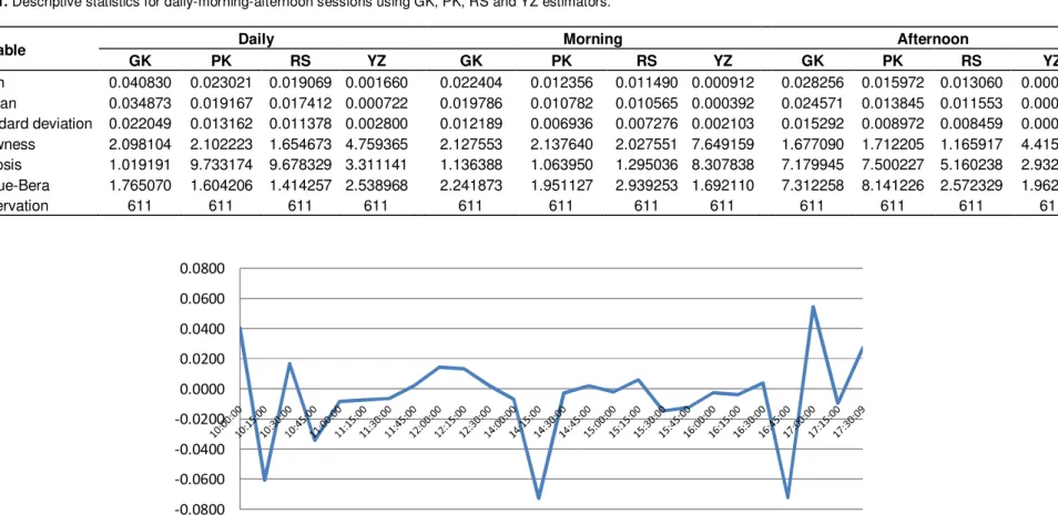
Figure 1 shows the 15-min mean return values for the ISE 100 Index and Figure 2 shows the standard deviation of intraday 15-min returns. The results are consistent with Bildik (2001) which indicates that stock returns follow a “W” shaped pattern over two separate trading sessions in a day. However, the pattern also creates a minor “W” shape in both sessions, but more significantly during the morning session. In other words, there is a “W” shaped pattern for the trading day in general and two minor “W” shaped patterns co-exist for the morning and afternoon sessions.
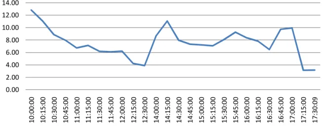
Opening and closing returns are significantly high both in daily values and for each of the morning and afternoon sessions. The volatility of the corresponding returns in each time period is shown in Figure 2.
Figure 2 specifically illustrates the different patterns of volatility of intraday 15-min returns. The average behavior indicates that right after the opening session the standard deviation shows a decreasing trend until the end of the first session. More significant fluctuations are observed in the afternoon session which is quite rational due to accumulated information flows during the intraday closing time between 12:30 and 14:15.
The results for Formulas 3, 4, 5, and 6 are presented in Figures 3, 4, 5, and 6 respectively for Parkinson’s, GK, YZ and RS volatility estimators for three different time periods: the daily, morning and afternoon sessions. The YZ estimator is clearly a more accurate estimator for estimating volatility in the existence of opening jumps. As mentioned earlier, the ISE is not continuous and has a midday break and also closes overnight. Information arriving during periods when the markets are closed often results in jumps in opening
Ulusoy et al. 7021
Table 1. Descriptive statistics for daily-morning-afternoon sessions using GK, PK, RS and YZ estimators.
Variable Daily Morning Afternoon
GK PK RS YZ GK PK RS YZ GK PK RS YZ Mean 0.040830 0.023021 0.019069 0.001660 0.022404 0.012356 0.011490 0.000912 0.028256 0.015972 0.013060 0.000479 Median 0.034873 0.019167 0.017412 0.000722 0.019786 0.010782 0.010565 0.000392 0.024571 0.013845 0.011553 0.000256 Standard deviation 0.022049 0.013162 0.011378 0.002800 0.012189 0.006936 0.007276 0.002103 0.015292 0.008972 0.008459 0.000682 Skewness 2.098104 2.102223 1.654673 4.759365 2.127553 2.137640 2.027551 7.649159 1.677090 1.712205 1.165917 4.415013 Kurtosis 1.019191 9.733174 9.678329 3.311141 1.136388 1.063950 1.295036 8.307838 7.179945 7.500227 5.160238 2.932561 Jarque-Bera 1.765070 1.604206 1.414257 2.538968 2.241873 1.951127 2.939253 1.692110 7.312258 8.141226 2.572329 1.962856 Observation 611 611 611 611 611 611 611 611 611 611 611 611 -0.0800 -0.0600 -0.0400 -0.0200 0.0000 0.0200 0.0400 0.0600 0.0800
Figure 1. Mean 15-min returns.
prices that differ significantly from the closing price of the prior trading sessions.
In terms of volatility, due to the fact that there are two opening jumps (morning and afternoon opening jumps) in the ISE, the YZ estimator proves to be a better estimator for estimating volatility for both opening jumps. Information arriving during periods when the markets are closed often results in opening prices which differ significantly from the closing prices of the prior trading sessions.
During the time when all Asian markets have closed and European markets are near to closing time, intraday ISE volatility increases throughout the U.S. trading session in local Turkish time. The news effect has clearly impacted the event horizon perceptions of corporate investors through internal volatility dynamics within the final stages of the ISE 100 Index afternoon session. The level of volatility signals a considerable upside pattern under the impact of the opening of the European markets in the morning
session, and again at the opening of the American markets. This phenomenon should be assessed as evidence that, despite existing knowledge about futures markets, traders in each region prefer to trade in their own time zones and explains the dynamics behind the higher market activity at the beginning and at the end of the regional trading ses-sions. This indicates a concrete signal for effective portfolio rebalancing. Volatility from the Asian market affects all other regions, and volatility for the Asian- European region
0.00 2.00 4.00 6.00 8.00 10.00 12.00 14.00 1 0 :0 0 :0 0 1 0 :1 5 :0 0 1 0 :3 0 :0 0 1 0 :4 5 :0 0 1 1 :0 0 :0 0 1 1 :1 5 :0 0 1 1 :3 0 :0 0 1 1 :4 5 :0 0 1 2 :0 0 :0 0 1 2 :1 5 :0 0 1 2 :3 0 :0 0 1 4 :0 0 :0 0 1 4 :1 5 :0 0 1 4 :3 0 :0 0 1 4 :4 5 :0 0 1 5 :0 0 :0 0 1 5 :1 5 :0 0 1 5 :3 0 :0 0 1 5 :4 5 :0 0 1 6 :0 0 :0 0 1 6 :1 5 :0 0 1 6 :3 0 :0 0 1 6 :4 5 :0 0 1 7 :0 0 :0 0 1 7 :1 5 :0 0 1 7 :3 0 :0 9
Figure 2. Standard deviation of intraday 15-min returns.
0 0.05 0.1 0.15 0.2 0 3 /0 9 /2 0 0 7 0 3 /1 0 /2 0 0 7 0 3 /1 1 /2 0 0 7 0 3 /1 2 /2 0 0 7 0 3 /0 1 /2 0 0 8 0 3 /0 2 /2 0 0 8 0 3 /0 3 /2 0 0 8 0 3 /0 4 /2 0 0 8 0 3 /0 5 /2 0 0 8 0 3 /0 6 /2 0 0 8 0 3 /0 7 /2 0 0 8 0 3 /0 8 /2 0 0 8 0 3 /0 9 /2 0 0 8 0 3 /1 0 /2 0 0 8 0 3 /1 1 /2 0 0 8 0 3 /1 2 /2 0 0 8 0 3 /0 1 /2 0 0 9 0 3 /0 2 /2 0 0 9 0 3 /0 3 /2 0 0 9 0 3 /0 4 /2 0 0 9 0 3 /0 5 /2 0 0 9 0 3 /0 6 /2 0 0 9 0 3 /0 7 /2 0 0 9 0 3 /0 8 /2 0 0 9 0 3 /0 9 /2 0 0 9 0 3 /1 0 /2 0 0 9 0 3 /1 1 /2 0 0 9 0 3 /1 2 /2 0 0 9 0 3 /0 1 /2 0 1 0 0 3 /0 2 /2 0 1 0
Daily Morning Afternoon
Figure 3. 15-min volatility using GK.
0 0.02 0.04 0.06 0.08 0.1 0.12 0 3 /0 9 /2 0 0 7 0 3 /1 0 /2 0 0 7 0 3 /1 1 /2 0 0 7 0 3 /1 2 /2 0 0 7 0 3 /0 1 /2 0 0 8 0 3 /0 2 /2 0 0 8 0 3 /0 3 /2 0 0 8 0 3 /0 4 /2 0 0 8 0 3 /0 5 /2 0 0 8 0 3 /0 6 /2 0 0 8 0 3 /0 7 /2 0 0 8 0 3 /0 8 /2 0 0 8 0 3 /0 9 /2 0 0 8 0 3 /1 0 /2 0 0 8 0 3 /1 1 /2 0 0 8 0 3 /1 2 /2 0 0 8 0 3 /0 1 /2 0 0 9 0 3 /0 2 /2 0 0 9 0 3 /0 3 /2 0 0 9 0 3 /0 4 /2 0 0 9 0 3 /0 5 /2 0 0 9 0 3 /0 6 /2 0 0 9 0 3 /0 7 /2 0 0 9 0 3 /0 8 /2 0 0 9 0 3 /0 9 /2 0 0 9 0 3 /1 0 /2 0 0 9 0 3 /1 1 /2 0 0 9 0 3 /1 2 /2 0 0 9 0 3 /0 1 /2 0 1 0 0 3 /0 2 /2 0 1 0
Daily Morning Afternoon Figure 4. 15-min volatility using Parkinson.
spills over into Europe where Turkey is impacted in terms of intra-day volatility due to its regional positioning for the morning session; consequently, volatility in the European region has some effects on America, and lastly, volatility in the America region has a significant
spillover effect on European and emerging markets in terms of portfolio flows and market capitalizations. These spillovers may explain why there is an intraday “W”-shaped return pattern and volatility jumps in the ISE during the period analyzed.
Ulusoy et al. 7023 0 0.0050.01 0.015 0.02 0.0250.03 0.035 0 3 /0 9 /2 0 0 7 0 3 /1 0 /2 0 0 7 0 3 /1 1 /2 0 0 7 0 3 /1 2 /2 0 0 7 0 3 /0 1 /2 0 0 8 0 3 /0 2 /2 0 0 8 0 3 /0 3 /2 0 0 8 0 3 /0 4 /2 0 0 8 0 3 /0 5 /2 0 0 8 0 3 /0 6 /2 0 0 8 0 3 /0 7 /2 0 0 8 0 3 /0 8 /2 0 0 8 0 3 /0 9 /2 0 0 8 0 3 /1 0 /2 0 0 8 0 3 /1 1 /2 0 0 8 0 3 /1 2 /2 0 0 8 0 3 /0 1 /2 0 0 9 0 3 /0 2 /2 0 0 9 0 3 /0 3 /2 0 0 9 0 3 /0 4 /2 0 0 9 0 3 /0 5 /2 0 0 9 0 3 /0 6 /2 0 0 9 0 3 /0 7 /2 0 0 9 0 3 /0 8 /2 0 0 9 0 3 /0 9 /2 0 0 9 0 3 /1 0 /2 0 0 9 0 3 /1 1 /2 0 0 9 0 3 /1 2 /2 0 0 9 0 3 /0 1 /2 0 1 0 0 3 /0 2 /2 0 1 0
Daily Morning Afternoon
Figure 5. 15-min volatility using YZ.
0 0.02 0.04 0.06 0.08 0.1 0.12 0 3 /0 9 /2 0 0 7 0 3 /1 0 /2 0 0 7 0 3 /1 1 /2 0 0 7 0 3 /1 2 /2 0 0 7 0 3 /0 1 /2 0 0 8 0 3 /0 2 /2 0 0 8 0 3 /0 3 /2 0 0 8 0 3 /0 4 /2 0 0 8 0 3 /0 5 /2 0 0 8 0 3 /0 6 /2 0 0 8 0 3 /0 7 /2 0 0 8 0 3 /0 8 /2 0 0 8 0 3 /0 9 /2 0 0 8 0 3 /1 0 /2 0 0 8 0 3 /1 1 /2 0 0 8 0 3 /1 2 /2 0 0 8 0 3 /0 1 /2 0 0 9 0 3 /0 2 /2 0 0 9 0 3 /0 3 /2 0 0 9 0 3 /0 4 /2 0 0 9 0 3 /0 5 /2 0 0 9 0 3 /0 6 /2 0 0 9 0 3 /0 7 /2 0 0 9 0 3 /0 8 /2 0 0 9 0 3 /0 9 /2 0 0 9 0 3 /1 0 /2 0 0 9 0 3 /1 1 /2 0 0 9 0 3 /1 2 /2 0 0 9 0 3 /0 1 /2 0 1 0 0 3 /0 2 /2 0 1 0
Satchell Daily Satchell Morning Satchell Afternoon
Figure 6. 15-min volatility using RS.
Another possible factor that could impact price movements is the contagion effect. Volatility transmission in a global market dynamic across different regions is mainly explained by intraregional volatility. It is common knowledge that many financial data series such as exchange rates and stock returns exhibit volatility clustering and different patterns of volatility transmission. Investors in a particular market show a biased behavior that has reacted rapidly and efficiently to information transferred from other similar markets, and they might still prefer to trade in their home markets. King and Wadhwani (1990) concluded that trading in one market has an influence on other market price movements as well. Chan et al. (1996) studied dually listed companies and pointed out that the daily volatility of European stocks traded in the U.S. market accrues in the mornings when compared to similar American stocks. On the other hand, there are also studies about intra-day patterns which claim results contrary to the contagion model, so it may also be possible for the ISE to be effected by trading patterns and volatility in U.S. and European markets (There is also a third set of factors which base their explanation on behavioral factors. According to behavioral finance literature, the psychology of investors and
markets in general might have an effect on forming intraday price movements and patterns. Mean reversion, price reversals, and noise traders in financial markets, as well as herding and informa-tional cascades and other behavioral factors can be an explanation for the observed intraday anomalies in the ISE in this study).
MODELING VOLATILITY AND EMPRICAL RESULTS
Modeling and forecasting volatility has been the subject of many empirical and theoretical studies. There are several motivations for such research targeting “the effi-ciency” of the econometric model. Volatility is often used as a “pure” measure of the risk of financial assets. From this perspective, researchers use volatility estimation and its forecasting results to price the related assets.
Here, GK study forms of YZ and RS estimators are taken and modeled into a GARCH (p,q) family. We were
Table 2. Regression results from the related volatility estimators. (1) (2) (3) (4) (5) (6) (7) (8) (9) (10) (11) (12) Constant -0.02** (-1.98) -0.003 (-0.56) 0.0078 (-0.69) -0.002 (-0.21) -0.019 (-2.88) -0.002 (-0.71) -0.004(-0.64) -0.0006(-0.08) -0.02** (-2.59) -0.01(-1.86) 0.03**(3.09) 0.02**(2.88) AR(1) -0.72** (-4.73) -0.71** (-5.88) -0.71** (-5.98) -0.71** (-6.00) -0.23** (-2.20) -0.36** (-9.64) -0.24**(-2.29) -0.37**(-9.81) -0.28(-0.88) MA(1) 0.58** (3.33) 0.58** (4.10) 0.57** (4.11) 0.57** (4.11) -0.15 (-1.46) 0.25(0.81) MA(3) -0.11 (-2.70) -0.11(-2.67) -0.11(-2.92) -0.12(-2.97) rs_morning 2.37** (2.01) 1.75** (3.31) rs_afternoon -2.10** (-3.37) yz_morning 6.82**(2.62) 3.59*(1.89) yz_afternoon -29.74**(-3.92) gk_morning 0.48(1.09) 0.23(0.77) gk_afternoon -1.27**(-3.78) par_morning 0.43(0.55) 0.08(0.15) par_afternoon -2.05**(-3.57)
Endogenous variables in (1), (2), (3) and (4): return_morning – return_afternoon (t-1); (5), (6), (7) and (8): return_morning – return_daily (t-1); (9), (10), (11) and (12): return_afternoon – return_morning; ** significance at 5% significance level; * significance at %10 significance level.
particularly interested in the relative explanatory power of volatilities obtained from econometric models and derived forms of YZ and RS. Table 2 shows the empirics of the model presented as:
)
,
,
,
,
(
Y
1YZ
RS
GK
PAR
f
Y
t=
t− (7)where Y is the return from the ISE100 index defined earlier. The lag values of Y are used as exogenous variables. YZ, RS, GK, and PAR are the related indicators of volatilities. All of these indicators which use the highest and lowest points of a daily price series, are a function of the vola-tility observed during the day and can provide improved volatility estimates. Although these range-based volatility estimators can be applied to any interval, the reliability of the estimate is de-pendent on the sampling frequency (Akay, 2010). A very distinctive feature of the model is its data source. Our data is divided mainly into three
groups and reflected in Formula 7. We run twelve separate regressions, three for each variable that covers morning and afternoon sessions in the same day, along with data covering whole day. The endogenous variable in the first four models is the difference between returns in the morning session at time t and the afternoon sessions at time t-1. This difference may capture the jumps in the morning session that might result from the news affects accumulated during the correspon-ding breaks.
The second set of regressions (5), (6), (7), and (8) are the volatility models where the endoge-nous variable is the difference between the returns in the morning session and the day–end at time t-1. Similarly, the return differences between the afternoon and morning sessions in the same day are presented in (9), (10, (11), and (12).
We begin our analysis by indicating that all regression models are stationary. This feature
improves the predictive power of the model and its parameters. The results in Table 2 clearly illustrate that YZ, RS, GK, and PAR measure of volatilities have mixed results with different magnitudes and directions of causation. The first set of regressions are all positive and YZ and RS are statistically significant. Although GK and PAR have positive effects on the return differences, they are statistically insignificant. The second set of results capture the effects of the volatilities on the return differences between the morning and the previous whole day. The parameters have the same pattern with positive impacts, with YZ and RS displaying statistically significant results.
Regressions of the differences in the return on the same day reveal a different picture inclusive of the negative effects of the volatilities of return differences. All the range-based volatilities display statistically significant results at a 1% level of significance. These findings indicate that the
Ulusoy et al. 7025
Table 3. Results from the GARCH-M model.
Mean equation (1) (2) (3) Constant -0.02 (-0.73) -0.015 (-0.87) 0.01 (0.59) t σ 0.17 (0.76) 0.13 (0.84) -0.15 (-0.62) AR(1) -0.72** (-4.99) 0.24** (-2.04) MA(1) 0.62** (3.74) -0.12 (-1.04) MA(3) -0.11** (-2.61) Variance equation Constant ω 0.001** (2.20) 0.0003** (2.31) 0.004** (3.52)
)
(
2 1 tα
ε
− 0.08** (2.92) 0.06** (3.50) 0.16** (3.51))
(
2 1 tβ
σ
− 0.86** (19.02) 0.91** (37.28) 0.61** (6.65)t-values are in parenthesis. endogenous variables: (1) return_morning – return_afternoon (t-1); (2) return_morning – return_daily (t-1); (3) return_afternoon – return_morning; ** significance at 5% significance level; * significance at 10% significance level.
accumulated news and related variables overnight have positive impacts on the return. Volatilities that may capture the news effects during the session breaks within the same day have an inverse impact on the related return variable. The results may support the view of Lockwood and Linn’s (1990) volatility study where return volatility decreases from the opening hour until early afternoon and increases subsequently and is consider-ably greater for intraday versus overnight periods. Along the same line, these results may also support the findings of Bildik (2001) which demonstrate that the opening and closing returns are large and positive, and volatility is higher at the openings and follows an L shaped pattern. The relatively higher mean and standard deviation at the opening sessions was generated by the accumulated overnight information and the closed-market effect (halt of trade) (LeBaron (1992) finds that the daily serial correlation of index returns is inversely related to the conditional volatility of index returns. Both the capital gain return of the SandP index and the total return of the value-weighted index from the Center for Research in Security Prices (CRSP) file exhibit this pattern. (1) LeBaron argues that the empirically inverse relation between serial correlation and conditional volatility is important for understanding asset price behavior and that it may enhance theoretical models of market micro-structure, learning, and information dissemination. He suggests that simple nontrading, specialist interventions, and news accumulation, each of which can cause index serial correlation, may be related to conditional volatility. (2) Thus, the relation between the two measures may be a function of economic factors).
Tables 3, 4, and 5 were derived from the GARCH model. The GARCH model allows the conditional
variance to be dependent upon previous lags, so that the conditional variance formula is in the simple case of:
2 1 2 1 1 0 2 − −
+
+
=
t t tα
α
ε
βσ
σ
. (8)This GARCH (1,1) model is based on the assumption that forecasts of variance changing in time depend on the lagged variance of the asset. An unexpected increase or decrease in the return at time t will generate an increase in the expected variability in the next period (Using the GARCH model it is possible to interpret the current fitted variance as a weighted function of a long term average value information about volatility during the previous period and the fitted variance from the model during the previous period). Table 3, as a variant of the approach presented in Table 2, gives the pure results from the GARCH-M model including the mean formula in the form of: t t 2 1 t 1 0 t
Y
u
Y
=
γ
+
γ
−+
γ
σ
+
(9)where the errors may follow MA(q) terms for the stationarity of the model. The estimates given in Table 3 are the realized set of results which will be used as a benchmark for testing the relative efficiency of the range-based volatilities that will be elaborated below. The GARCH-M results in Table 3 illustrate that the variance (or standard deviation) of the model does not have statis-tically significant effects on the return differences while the GARCH model illustrates a highly significant parameter estimate.
These results may suggest that range-based volatility measures may be substituted for the classical measure
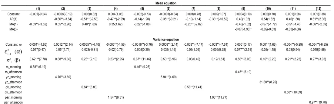
Table 4. Regression results from GARCH model including RS and YZ measures. Mean equation (1) (2) (3) (4) (5) (6) (7) (8) (9) (10) (11) (12) Constant -0.001(-0.24) -0.0008(-0.19) 0.003(0.82) 0.004(1.08) -0.002(-0.73) -0.0001(-0.64) 0.001(0.78) 0.002(1.07) 0.0004(0.10) 0.002(0.70) 0.001(0.28) 0.001(0.38) AR(1) -0.66**(-3.84) -0.51**(-2.53) -0.47**(-2.29) -0.14(-1.20) -0.35**(-9.21) -0.10(-1.14) -0.33**(-10.52) 0.40(1.02) 0.54(1.62) 0.46(1.30) 0.61**(2.36) MA(1) -0.59**(-3.52) 0.55**(2.90) 0.40*(1.83) 0.35(1.62) -0.22*(-1.88) -0.25**(-2.82) -0.40(-1.02) -0.57*(-1.72) -0.51(-1.43 -0.66**(-2.69) MA(3) -0.07(-1.90)* -0.02(-0.83) -0.03(-0.88) Variance equation Constant ω -0.001*(-1.65) 0.0012**(2.14) -0.0055**(-4.40) -0.005**(-4.56) -0.0016**(-3.76) 0.0008**(2.14) -0.003**(-7.17) -0.003**(-7.61) 0.0001(0.17) 0.001*(1.66) -0.004**(-5.99) -0.004**(-6.85)
)
(
2 1 tα
ε
− 0.017(0.47) 0.05*(1.71) -0.023(-0.81) -0.02(-0.79) 0.005(0.20) 0.037(1.15) 0.03(1.09) 0.009(0.28) 0.077**(2.51) -0.02(-1.15) 0.03(0.94) 0.019(0.56) ) ( 2 1 t β σ− 0.62***(7.78) 0.68**(9.60) 0.23**(2.10) 0.23**(2.25) 0.67**(11.46) 0.53**(6.96) 0.03(0.40) 0.12(1.51) 0.56**(8.03) 0.16**(2.20) 0.21**(2.23) 0.27**(3.03) rs_morning 0.68**(6.19) 0.46**(9.25) rs_afternoon 0.45**(6.19) yz_morning 4.76**(3.69) 5.94**(4.69) yz_afternoon 31.68**(8.25) gk_morning 0.84**(8.83) 0.58**(11.41) gk_afternoon 0.58**(10.69) par_morning 1.54**(8.31) 1.03**(11.77) par_afternoon 0.97**(10.70)Endogenous variables in (1), (2), (3) and (4): return_morning – return_afternoon (t-1); (5), (6), (7) and (8): return_morning – return_daily (t-1); (9), (10), (11) and (12): return_afternoon – return_morning; ** significance at 5% significance level; * significance at 10% significance level.
of the variation. In other words, variance differences at the beginning and at the end of the trading day, along with periods between the ses-sions, may be better presented with range-based volatility measures.
The estimated parameter values given in Table 4 indicate another dimension of the volatility efficiency. In particular, we include the related RS, YZ, GK, and PAR measures of range-based volatility in the variance equation portion of the GARCH model to observe the explanatory power of these measures on the volatility of the model.
The same set of twelve regression models were run again. Again for all the models estimated, we first satisfied the stationary conditions. The GARCH portion of the model achieved promising results for all range-based estimates. For all twelve regressions, we obtained statistically signi-ficant results at the 1% level of significance, but with different magnitudes. The results revealed some notable implications. As in the previous cases, YZ had a greater effect on the volatility of the model in magnitude. Even though the effects of all other range-based estimates on the variance
of the model did not vary too much for all cases, YZ differed significantly. The effect of YZ was much greater once the model covered the return differences within two sessions within the day. Given the fact that the data covered a period that was financially unsound, we expected that the return volatility would decrease from the opening hour until the early afternoon and subsequently increase and be considerably greater for intraday versus overnight periods. In other words, the news effect and the speculative actions within the day may be greater than that of overnight periods.
Although the explanatory power of range-based volatilities are apparent, one may be concerned about the day-of-the week effects on the volatility of the model simply because of the market structure of the ISE. Considering that settlements take place on the day T+2, buying on Thursdays and Fridays simply extends the transaction to T+4 (adding the weekend), allowing investors to earn two extra days of interest in the repo market. This could well create an upward market on Thursdays and Fridays (buying takes place) and a downward market on Mondays and Tuesdays as selling will probably take place on these two days. Table 5 illustrates such a set of regression results from the same GARCH models. The day dummies, representing the days of a week, are included in each model to capture the remaining jumps in the volatility of models. Again, we paid particular attention to the variance equation (For all the set of regression models in Tables 2 to 5, we ran an additional regression equation where the mean equation covers the day dummies. We eliminated one of the dummies to avoid the perfect multicollinearity problem. Almost all the results show that day-of the week effects are statistically insignificant. The results are expected for the period of data we cover in the analysis. In other words, the day-of-the-week effect does not have expla-natory power on mean return differences when the time period is financially unstable).
The results show that the magnitude and the signs of range-based volatility measures do not change significantly once dummies are included. Dummies may capture the volatility effects of the day-of-the-week in different aspects. Comparing these twelve regression models, dummies reveal a more prominent status in the second set of results from (6) to (8), excluding the model (7) in Table 5. These results illustrate, in general, that return differences from the previous whole day enhance the explanatory power of the day-dummies. Most of the
dummies in Table 5 from formula (5) to (8) are statistically
significant at a 1% level of significance. There are a few issues to emphasize on this point. First, dummies may help capture anomalies along with the range-based estimates of volatilities. In other words, they are comple-mentary measures to these volatility indicators. Second, the inclusion of dummies enhances the explanatory power of the range-based estimators provided that the dummies are statistically significant. Additionally, results may be the indicators of news effects for the reason that the return differences are expressed in the form of “morning at time t and the previous whole-day” (Thursday has some special implications for the Turkish Stock Exchange Market. Once portfolio investors decide to buy
additional assets from the market on Thursdays, payments
are delayed until coming Monday. This may well change the behavior of the return model, particularly for finan-cially unstable periods because 4 to 5 days of payment delay may provide additional opportunities for investors
Ulusoy et al. 7027
who are closer to the market information set, relative to others).
EFFICIENCY OF RANGE-BASED VOLATILITIES
Here, we follow the path of the pioneering study done by Akay et al. (2010). We focused exclusively on all of the range-based volatility measures to determine whether the method we apply provides volatility estimates consistent with the theoretical volatility of the Istanbul Stock Exchange Market. As in Akay (2010), to examine the efficiency of range-based volatility estimators, we take the GARCH estimates as a benchmark measure of realized volatility and compare its RMSE (Root-Mean-Square-Errors) with that of range-based volatility measures. Specifically, the 12 regressions of returns explained earlier were run to obtain the standard deviation in the following form:
t t t
r
=
α
0+
α
1σ
+
ε
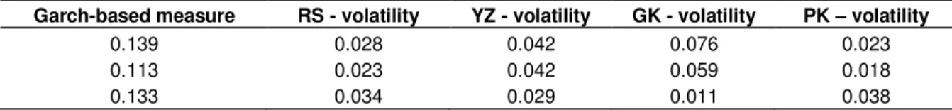
(10)where, r is the return difference defined above, ε is the error term, and σ are the range-based volatility measures (YZ, RS, GK, and PAR). We estimated an additional 12 regression models to obtain the ARCH and GACRH components of each measure as in Formula (8). Table 6 shows the results of the RMSE calculated from these ARCH/GARCH components of such regression equations.
Table 6 illustrates that all of the range-based measures are more efficient than the GARCH measure of volatility measures since their RMSEs are smaller. In the first and the second sets of regressions, PK is the most efficient. It is the least efficient volatility measure for the last group of models. The last group contains the intraday return differences; GK is the most efficient and PK is the least efficient measure of volatility among the range-based measures.
Following Akay (2010), we may state that this may occur for two reasons: one methodological and the second as a result of the nature of the market. Recall that the GK method uses the open and closing observations as well as high and low observations, whereas the Parkinson method only uses the high and low values. The first possible explanation is the method by which we obtained the open and close observations employed in this article as explained in the data section. Secondly, Bali and Weinbaum (2005) examined the SandP 500 index futures and three exchange rates, revealing that the previous trade and thus the opening tend to have more information because the markets are homoge-neous. Additionally, there is also evidence from the federals funds market (Cyree and Winters, 2001), exchange rate markets (Ederington and Lee, 1993) and other stock markets, for example, Australian stock
Table 5. Regression results from the GARCH model including RS and YZ measures and day-of-the week effect. Mean equation (1) (2) (3) (4) (5) (6) (7) (8) (9) (10) (11) (12) Constant -0.0006(-0.14) -0.001(-0.30) 0.003(0.79) 0.003(0.84) -0.001(-0.609 -0.003(-1.26) 0.001(0.72) 0.001(0.84) 0.0003(0.08) 0.002(0.58) 0.001(0.39) 0.002(0.56) AR(1) -0.45**(-1.97) -0.65**(-4.53) -0.46**(-2.08) -0.44**(-1.99) -0.17(-1.59)* -0.32**(-9.21) -0.12(-1.31) -0.33**(-11.77) 0.34(0.85) 0.54*(1.65) 0.59**(2.31) 0.53(1.63) MA(1) 0.32(1.31) 0.54**(2.67) 0.34(0.23) 0.32(1.38) -0.18(-1.69) -0.23**(-2.53) -0.35(-0.86) -0.57*(-1.75) -0.64**(-2.64) -0.56*(-1.74) MA(3) -0.08**(-2.03) -0.03(-0.91) -0.03(-0.88) Variance equation Constant ω -0.006**(-2.88) 0.0001(0.61) -0.005**(-3.53) -0.007**(-11.59) -0.004**(-6.01) 0.0008(0.93) -0.003**(-6.77) 0.001(0.70) -0.001(-0.61) 0.001(1.62) -0.004**(-2.78) -0.005**(-3.94) ) ( 2 1 t α ε− 0.01(0.45) 0.05*(1.72) -0.02(-0.87) -0.03(-1.46) -0.003(-0.12) 0.06(1.54) 0.01(0.41) -0.01(-0.40) 0.097**(2.93) -0.02(-1.01) 0.03(0.88) 0.08(0.23) ) ( 2 1 t β σ− 0.59**(6.99) 0.68**(9.26) 0.23**(2.19) 0.23**(2.80) 0.53**(7.24) -0.01(-0.51) 0.09(1.02) 0.15(1.38) 0.51**(6.32) 0.15**(1.96) 0.20**(2.00) 0.41**(5.72) rs_morning 0.78**(6.13) 0.59**(8.34) rs_afternoon 0.45**(4.80) yz_morning 4.74**(3.46) 13.70**(7.59) yz_afternoon 31.13**(7.86) gk_morning 0.85**(8.24) 0.59**(11.13) gk_afternoon 0.59(8.83) par_morning 1.68**(9.01) 0.94**(9.00) par_afternoon 0.87**(10.19) Dmon 0.005*(1.71) 0.001(0.51) 0.0005(0.285) 0.001(1.00) 0.002**(2.28) 0.002**(2.00) -0.0007(-0.93) -0.006**(-2.10) -0.0008(-0.30) -0.001(-0.92) -0.0002(-0.11) -0.0006(-0.31) Dtue 0.003(1.28) -0.002(-0.76) 0.0007(0.44) 0.001(1.38) 0.003**(3.54) 0.001(1.53) 0.0005(0.26)) -0.005**(-1.98) 0.003(1.27) -0.000007(-0.04) -0.0004(-0.28) 0.0005(0.30) Dwes 0.004(1.54) 0.001(0.48) -0.0005(-0.26) 0.0002(0.14) 0.003**(2.70) 0.004**(2.39) -0.0005(-0.67) -0.005**(-2.11) 0.001(0.37) -0.0006(-0.40) -0.0002(-0.13) 0.0009(0.58) Dthur 0.008**(2.38) -0.0008(-0.24) 0.0009(0.48) 0.001(0.75) 0.006**(4.15) 0.003**(2.54) -0.0004(-0.59) -0.005**(-2.33) 0.005*(1.78) -0.001(-0.82) -0.0001(-0.07) 0.001(0.56) Endogenous variables in (1), (2), (3) and (4): return_morning – return_afternoon (t-1); (5), (6), (7) and (8): return_morning – return_daily (t-1); (9), (10), (11) and (12): return_afternoon – return_morning; ** significance at 5% significance level; * significance at 10% significance level.
markets (Kalev and Pham, 2009), that the observed patterns are rational responses to market structure and/or information arrivals. This market structure may result in inter-day sessions creating information flow. This suggests that PK volatility measures should work better in the first two settings as seen in Table 6. Whatever the for-mat of the return equation, range-based volatilities
are more efficient compared to those of the conventional measure. a more heterogeneous environment than intra-day
These findings support the view that range-based measures reduce the effect of micro-structure noise. As in Akay (2010), we suggest that range-based methods not only reduce such a noise but are also able to categorize the different
volatility measures along with the regular measure.
Conclusion
This study has utilized an analytical approach regarding the dynamics of Turkey’s ISE 100 Index intraday return and price volatility during the
Ulusoy et al. 7029
Table 6. Relative efficiency of the estimators by comparing the RMSEs, using a Garch-based measure as the benchmark of realized volatility.
Garch-based measure RS - volatility YZ - volatility GK - volatility PK – volatility
0.139 0.028 0.042 0.076 0.023
0.113 0.023 0.042 0.059 0.018
0.133 0.034 0.029 0.011 0.038
The rows correspond to the RMSE of the regression equations: (return_morning – return_afternoon (t-1)); (return_morning – return_daily (t-1)); and (return_afternoon – return_morning), respectively.
period of financial turmoil which lasted from August 2007 to February 2010.
This study makes contributions in three ways to the literature on the financial market and its behavior. Firstly, we employed unique data on returns in the ISE market. Secondly, the study explored the behavior of the ISE market by applying four different measures of volatility: YZ, RS, GK, and PK. Thirdly, we tested the relative efficiency of these volatility measures by establishing realized volatility as a benchmark.
The empirical results are consistent with the previous literature; there is a “W”-shaped pattern for the trading day in general and two minor “W” shape patterns exist for the morning and afternoon sessions. It was also observed that on average trading risks are highest at the start and end of the day.
Estimated results illustrate that all range-based volatility measures have some explanatory power concerning ISE market volatility. The findings are relevant for establishing the accuracy and relevance of the extreme value volatility estimate. We show that these measures are also highly efficient relative to benchmark ARCH/GARCH estimates. This supports the view in the literature that range-based volatility measures reduce the effect of microstructure noise.
These results coincide with the mainstream research in this area. We find strong evidence that economic volatility and trading process volatility can be decomposed and investigated simultaneously using opening, closing, high, and low values within the daily trading sessions. The measures investigated cover these types of information and decomposition. Further research should test and compare the YZ estimator with other developing and developed security markets.
REFERENCES
Akay O, Griffiths MD, Winters DB (2010). On the Robustness of Range-Based Volatility Estimators. J. Financ. Res., 33: 179-199.
Alizahdeh S, Brandt W, Diebold X (2002). Range-based estimation of stochastic volatility models. J. Financ., 57: 1047-1091.
Aitken M, Brown P, Walter T (1993). Intraday Patterns in Returns, Trading Volume, Volatility and Trading Frequency on SEATS. University of Western Australia Working Paper.
Aydoğan K, Booth G (2003). Calendar anomalies in the Turkish foreign exchange markets. Appl. Financ. Econ., 13: 353-360.
Bali T, Weinbaum G (2005). A comparative study of alternative extreme-value volatility estimators. J. Futures Mark., 25(9): 873-892. Baillie R, Bollerslev T (1990). Intra-Day and Inter-Market Volatility in
Foreign Exchange Rates. Rev. Econ. Stud., 58(3): 565-585.
Beckers S (1983). Variances of Security Price Returns Based on High, Low and Closing Prices. J. Bus., 56(1): 97-112.
Bildik R (2004). Are Calendar Anomalies Still Alive?: Evidence from Istanbul Stock Exchange. Reterieved from SSRN: http://ssrn.com/abstract=598904 on February 01, 2010.
Bildik R (2001). Intra-day seasonalities on stock returns: evidence from the Turkish Stock Market. Emerg. Mark. Rev., 2(4): 387-417. Chan K, Christie C, Stulz R (1996). Information, trading and stock
returns: lessons from dually listed securities. J. Bank. Financ., 20: 1161-1187.
Chang RP, Fukuda T, Rhee SG, Taakano M (1993). Intraday and interday behavior of the TOPIX. Pasific-Basin Financ. J., 1: 67-95. Cyree KB, Winters DB (2001). An Intraday Examination of the Federal
Funds Market: Implications for the Theories of the Reverse-J Pattern. J. Bus., 74(4): 535-556.
Demirer R, Baha M (2002). An Investigation of the Day-of-the-Week Effect on Stock Returns in Turkey. Emerg. Mark. Financ. Trade, 38(6): 47-77.
Ederington LH, Lee JH (1993). How Markets Process Information: News Releases and Volatility. J. Financ., 48(4): 1161-1191.
Edwards FR (1988). Futures Trading and Cash Market Volatility: Stock Index and Interest Rate Futures. J. Futures Mark., 8(4): 421-439. Foster FD, Viswanathan S (1990). A Theory of Interday Variations in
Volumes, Variances and Trading Costs in Securities Markets. Rev. Financ. Stud., 4: 595-624.
Gerety MS, Mulherin JH (1992). Trading Halts and Market Activity: An Analysis of Volume at the Open and the Close. J. Financ., 47: 1765-84.
Garman M, Klass M (1980). On the estimation of security price volatilities from historical data. J. Bus., 53(1): 67-78.
Harris L (1986). A transaction data study of weekly and intradaily patterns in stock returns. J. Financ. Econ., 16(1): 99-117.
Harris L (1989). SandP 500 Cash Stock Price Volatilities. J. Financ., 44(5): 1155-75.
Hong H. Wang J (2000). Trading and Returns under Periodic Market Closures. J. Financ., 55(1): 297-354.
Istanbul Stock Exchange.Retrieved from Istanbul Stock Exchange on February 16, 2010: http://www.ise.org/Markets/StockMarket.aspx Jain PC, Gun-Ho J (1988). The Dependence between Hourly Prices
and Trading Volume. J. Financ. Quant. Anal., 23:269-283.
Kalev PS. Pham LT (2009). Intraweek and intraday trade patterns and dynamics. Pacific-Basin Financ. J., 17:547-564.
King M, Wadhwani S (1990). Transmission of volatility between stock markets. Rev. Financ. Stud., 3: 5-33.
LeBaron B (1992). Some relations between volatility and serial correlations in stock market returns. J. Bus., 65: 199-219.
Lockwood LJ, Linn SC (1990). An Examination of Stock Market Return Volatility During Overnight and Intraday Periods, 1964-1989. J. Financ., 45(2): 591-601
Lowengrub P, Melvin M (2002). Before and after international cross-listing: an intraday examination of volume and volatility. J. Int. Financ. Mark. Inst. Money, 12(2): 139-155.
McInish HT, Wood RA (1990a). A transactions data analysis of the variability of common stock returns during 1980-1984. J. Bank. Financ., 14(1): 99-112.
McInish HT, Wood RA (1990b). An analysis of transactions data for the Toronto Stock Exchange : Return patterns and end-of-the-day effect. J. Bank. Financ., 14(2-3): 441-458.
Niemayer J, Sanda P (1993). The Market Microstructure of the Stockholm Stock Exchange. Stockholm School of Economics Working Paper.
Parkinson M (1980). The extreme value method for estimating the variance of the rate of return. J. Bus., 53: 61-68.
Rogers L, Satchell S (1991). Estimating variance from high, low and closing prices. Ann. Appl. Prob., 1: 504-512.
Smirlock M, Starks L (1986). Day-of-the-Week and Intraday Effects in Stock Returns. J. Financ. Econ., 17: 197-210.
Stoll HR, Whaley RE (1990). Stock Market Structure and Volatility. Rev. Financ. Stud., 3: 37-71.
Wiggins JB (1991) . Empirical Tests of the Bias and Efficiency of the Extreme-Values Variance Estimator for Common Stocks. J. Bus., 64(3): 417-432.
Wood RA, McInish TH, Ord JK (1985). An Investigation of Transactions Data for NYSE Stocks. J. Financ., 40(3): 723-39.
Yang D, Zhang Q (2002). Drift independent volatility estimation based on high, low, open and close prices. J. Bus., 73: 477-491.
Yadav PK, Pope PF (1992). Intraweek and intraday seasonalities in stock market risk premia: cash and futures. J. Bank. Financ., 16: 233-270.