Optimal representation and processing of optical signals in quadratic-phase systems

(1)

Invited Paper

Optimal representation and processing of optical signals in

quadratic-phase systems

Sercan Ö. Ar

_ık

a,n

, Haldun M. Ozaktas

b

a

Stanford University, Department of Electrical Engineering, 94305 Stanford, CA, USA b_{Bilkent University, Department of Electrical Engineering, 06800 Bilkent, Ankara, Turkey}

a r t i c l e i n f o

Article history:

Received 6 November 2015 Received in revised form 11 December 2015 Accepted 12 December 2015 Available online 24 December 2015 Keywords:

ABCD systems Quadratic-phase systems Fourier optics

Sampling

Fractional Fourier transform Linear canonical transform

a b s t r a c t

Opticalfields propagating through quadratic-phase systems (QPSs) can be modeled as magnified frac-tional Fourier transforms (FRTs) of the input field, provided we observe them on suitably defined spherical reference surfaces. Non-redundant representation of thefields with the minimum number of samples becomes possible by appropriate choice of sample points on these surfaces. Longitudinally, these surfaces should not be spaced equally with the distance of propagation, but with respect to the FRT order. The non-uniform sampling grid that emerges mirrors the fundamental structure of propagation through QPSs. By providing a means to effectively handle the sampling of chirp functions, it allows for accurate and efficient computation of optical fields propagating in QPSs.

1. Introduction

Quadratic-phase systems (QPSs), also known as _ﬁrst-order optical systems or ABCD systems, are a very general family of optical systems encompassing arbitrary concatenations of various components such as thin lenses and sections of free space in the Fresnel approximation, as well as quadratic graded-index media

[1–4]. Mathematically, QPSs are referred to as linear canonical transforms [5,7,6,8–11]. In this paper, we derive the optimal sampling grid for this general family. This non-redundant grid of sample points mirrors the physical structure of QPSs and enables their accurate and fast simulation. The fractional Fourier transform (FRT) plays a fundamental role in the analysis of QPSs. We also analyze the evolution of spatial information along the longitudinal direction and show that the spherical reference surfaces should be equally spaced with respect to the fractional Fourier transform order. Our results are relevant to work on both sampling and fast computation of lightﬁelds propagating through quadratic-phase systems[12–26].

2. Decomposition of propagation in quadratic-phase systems

We will use ^f x and( ) F^(σx)to represent an optical signal in the

space domain and the frequency domain, respectively. Although we work with functions of a single variable for sake of simpler analysis, our results can be generalized to two dimensions. It will be useful to introduce dimensionless variables u¼x/s and μ= sσx

for space and frequency, where s is a scaling parameter with units of length. We now deﬁne ^f x( ) ≡ (1/ s f u) ( )and F^(σx) ≡ s F( )μ.

The functions f(u) and F( )μ are the space- and frequency-domain functions that take dimensionless arguments. More information on this dimensional normalization process may be found in[1].

The FRT can be viewed as the“fractional operator power” of the common Fourier transform (FT). One way of deﬁning the ath order FRT of a function f(u), which we denote by fa(u), is

∫

π π π π _{( )}

( ) = [ ( ( ) − ′ ( ) + ′ ( ))] ( ′) ′

−∞ ∞

1

f ua Aa expi u2cota /2 2uucsca /2 u2cota /2 f u du

See[1]for subtleties in the deﬁnition of fractional operator powers as well as alternative ways of deﬁning the FRT. Here

π

= − ( )

Aa 1 icota /2 . When a¼1, we obtain the common FT, so that the FRT can be seen as a generalization of the common FT. Viewed in the space–frequency plane (phase space), the act of taking the FRT of a signal results in a α= a /2π rotation of its Wigner distribution. This can be expressed as a relation between the Wigner distribution of f(u) and the Wigner distribution of fa(u)

as follows[27]:

μ α μ α α μ α

( ) = ( − + ) ( )

Wfau, W uf cos sin ,usin cos . 2

Quadratic-phase systems (QPSs) are unitary. The input ^f x( ) leads to an output g x^ ( )given by

Contents lists available atScienceDirect

journal homepage:www.elsevier.com/locate/optcom

Optics Communications

n_{Corresponding author.}

E-mail addresses:soarik@stanford.edu(S.Ö. Arık),

(2)

∫

β ^ ( ) = ^( ′) ′ ( ) π π α β γ − −∞ ∞ ( − ′+ ′ ) g x e e f x dx . 3 i/4 i x2 2xx x2

They are often characterized by the ABCD parameters which satisfy − =

AD BC 1 and are deﬁned as

γ β β β γα β α β = = = − + = ( ) A , B 1, C , D . 4

Consider a quasi-monochromatic optical signal with wavelength

λ

. Fresnel diffraction and passage through a thin lens are special kinds of QPSs. For Fresnel propagation over a distance d, we have

= =

A D 1, C¼0, andB=λd. For a thin lens with focal length f we have A=D=1, B¼0, and C= −1/ .λf

Quadratic-phase systems have many decompositions. A de-composition is the breaking down of the system into consecutive simpler parts. One of the possible decompositions involves three stages. Thefirst is a FRT operation, the second is a magnification operation, and thefinal stage is a chirp multiplication operation

[28–32]: ⎛ ⎝ ⎜ ⎞ ⎠ ⎟ ⎛ ⎝ ⎜ ⎞ ⎠ ⎟ π λ ^ ( ) = ( ) π λ− π g x e e sM i x R f x sM 1 exp . 5 i d ia a 2 / /4 2

Here a, M, and R are deﬁned through

⎛ ⎝ ⎜ π⎞_⎠⎟= ( ) a s B A tan 2 1 , 6 2 π = + = ( ) _{( )} M A B s A a cos /2 , ₇ 2 2 4 λR = s + + ( ) B A A B s C A 1 1 / / . 8 4 2 2 4

The ambiguity in inverting the tangent in Eq. (6)should be re-solved by choosing a in 0<a<2 for B>0 and in 2<a<4 for

<

B 0. We will make a number of observations on these equations. First, we note that the unit-magnitude _ei2πd/λ_e−iaπ/4 _{terms are} constant and unimportant for our purposes. Furthermore, the chirp multiplication term can be eliminated, if we decide to ob-serve the output not on a planar surface, but on a spherical re-ference surface with radius as given by the value of R above. In this case, we observe a magnified version of the FRT of the input, with the magnification given by the value of M above. A final note is

that, Eq.(5)is valid no matter what we choose s to be. This de-composition will constitute the basis for our derivation of the optimal sampling grid.

3. Transverse sampling spacing

A discussion of sampling often begins with assumptions on the extent of the signals in both space and frequency, the latter often called the bandwidth. An alternative approach is to specify the extent of the signals in the space–frequency plane. Our beginning assumption will be to specify the space–frequency region to which the signal is confined. Here, “confined” means that a sufficiently large percentage of the total energy is contained in that region.

We will take the z¼0 plane as our input plane. We assume that the space–frequency region of conﬁnement of the input signal at this plane is an ellipse with diameters denoted by Δx and Δσx

(Fig. 1(a)). Note that this implies that the space extent of the signal isΔxand that the frequency extent of the signal isΔσx. How many

samples are needed to represent the signal? The sampling theo-rem of Nyquist–Shannon requires a sampling interval of 1/Δσx.

Over a spatial extent of Δx this means N= Δ (x/ 1/Δσx) = Δ Δx σx

samples. This is known as the space–bandwidth product. The same derivation can be repeated in dimensionless coordinates. Now the ellipse diameters (and thus also the space and frequency extents) areΔx s/ and sΔσx, which lead to the same value of N. The space–

bandwidth product is invariant under scalings and does not de-pend on s.

We now consider a QPS between the z¼0 and z¼d planes characterized by the parameters ABCD. For example, in a system made up of lenses separated by sections of free space, these ABCD parameters will depend on the focal lengths and locations of the lenses. We willﬁrst determine the spatial extent of the output signalg x^ ( )observed at z¼d, given an input signal^f x at z( ) ¼0. It is known that the Wigner distributions of ^f x and( ) g x^ ( )have the following relationship[1,33–36]:

σ σ σ

^

( ) = ^ ( − − + ) ( )

W xg , x W Dxf B x, Cx A x . 9

Based on our assumption that the initial space–frequency dis-tribution of the signal is well-conﬁned to an elliptical region with diametersΔxandΔσx, and using Eq.(9), it is possible to show that

the output space–frequency distribution will have a spatial extent

σ Δ ″ =x Δx D2 2+ Δ x2 2B , (10)

Δσ

_x

Δσ

_x

Δσ

_x

Δx

_Δx

(a)

(b)

(c)

x

σ

_x

σ

_x

σ

_x

Fig. 1. The space–frequency ellipses show the approximate region of conﬁnement of the (a) input signal, (b) output signal on the planar reference surface, and (c) output signal on the spherical reference surface (s= Δ Δx/ σx, which is the optimal value).

(3)

and a frequency extent

σ σ

Δ x″ = Δx C2 2+ Δ x2 2A . (11)

The derivation of these results are similar to those in[37]and are thus not repeated. On the output plane, the space–bandwidth product is N″ = Δ ″Δ ″x σx . It can be shown that we always have

″ ≥

N N, with equality in the trivial case B=C=0 and A=1/D

(simple scaling system). We have used double primes since we are saving the use of single primes for the output on the spherical reference surfaces. The linearly distorted region of conﬁnement on the output plane at z¼d is illustrated inFig. 1(b).

We now wish to obtain an expression for the spatial extent Δ ′x

of the outputﬁeld on the spherical reference surface. We refer to Eq.(5). First we choose a scale parameter s and map the ellipse enclosing most of the signal energy, into a dimensionless space– frequency plane. Here, the diameters areΔx s/ and sΔσx. Now, we

apply a FRT of order a, which results in a rotation by an angle

α= a /2π . Using Eq.(2), weﬁnd that the rotated ellipse has a spatial extent of ( Δs σxsinα) + (Δ2 xcos /αs)2, in dimensionless co-ordinates. To express this in dimensional coordinates, we multiply by s. Finally, we multiply with the magniﬁcation M to obtain the spatial extent of the output signal on the spherical reference sur-face:

σ α α

Δ ′ =x M ( Δs2 xsin ) + (Δ2 xcos )2. (12)

Following a similar argument, we can derive the spatial frequency extentΔ ′σxof the output signal on the spherical reference surface

as ( Δs σxcosα) + (Δ2 xsin /αs)2. Dividing by s to express in di-mensional coordinates, andﬁnally dividing by the magniﬁcation M, we obtain σ σ α α Δ ′ = (Δ ) + (Δ ) ( ) M x s 1 cos sin / . 13 x x 2 2 2

Now, it is possible to obtain the space–bandwidth product on the spherical reference surface: N′ = Δ ′Δ ′x σx from the above

ex-pressions:

( )

σ α α σ α α α α

′ = [ (Δ ) + Δ Δ ( + ) + Δ ] 14

N s4 x4sin2 cos2 x2 x2sin4 cos4 x4sin2 cos2 /s4 1/2.

Calculating the minimum value of Eq.(14)by equating its de-rivative with respect to s to 0, weﬁnd that the minimum occurs at

σ

= Δ Δ ( )

s x/ x. 15

With this value of s, we always haveN′ =N, regardless of ABCD. In

other words, this choice of s allows the output signal to be fully re-presented on the spherical reference surface, with the same number of samples as the input signal. In contrast, sinceN″is equal to N only for very special values of ABCD, the representation of the signal on the planar output plane would require a greater number of sam-ples than information theoretically necessary. Thus, the use of spherical reference surfaces allows non-redundant representation of signals with the minimum possible number of samples. Since this is possible if and only if the scale parameters= Δ Δx/ σx, we

refer to this value of s as the natural scale parameter. What is special about this value of s? It makes the spatial extentΔx s/ and the frequency extent sΔσx in dimensionless phase-space both

equal to Δ Δx σx = N. For this value of s, the ellipse is reduced to

a circle with diameter N. A rotated circle is still the same circle. So the FRT operation, whose effect in phase space is to rotate, does not change this circular region in any way. The consequence of this is that in dimensional coordinates, the output space extent is nothing more complicated than the input space extent multiplied with M, and the output frequency extent is nothing more than the input frequency extent divided by M. This leaves the space– bandwidth product unchanged.

These observations can also be seen fromFig. 1(c), which shows the space–frequency region-of-conﬁnement of the signal on the spherical reference surface. With the natural scale parameter, not only are the area of the ellipses inFig. 1(a) and (c) (and the area of their bounding rectangles) equal, but the space–bandwidth pro-duct and thus number of samples for the region inFig. 1(c) is equal to that inFig. 1(a). This becomes possible because the natural scale parameter equates the vertical and horizontal extents of the el-lipse in dimensionless coordinates, reducing it to a circle. Conse-quently, no matter how much the space_{–frequency region is} ro-tated by the FRT operation, the circle remains a circle and upon going back to dimensional coordinates we obtain an ellipse with axes aligned with the space and frequency axes as inFig. 1(c). In contrast, the sheared space–frequency region inFig. 1(b), although having an area equal to the area of the region inFig. 1(a), exhibits a space–bandwidth product which is larger, requiring a greater number of samples. In other words, shearing leads to a space– bandwidth product and number of samples needlessly greater than the true number of degrees of freedom of the signal (given by the area of the region, which is invariant). Use of the natural scale parameter on the appropriate spherical reference surface avoids shearing and thus keeps the number of samples equal to the true number of degrees of freedom of the signal.

The opticalfield on the output spherical reference surface is simply related to thefield on the input plane through a magnified FRT. If we choose the natural scale parameter, the magni_fication has a simple effect. It increases the spacing of the samples by a factor of M from1/ΔσxtoM/Δσx, without affecting their values. We

refer to these spherical reference surface samples as the natural sampling grid. Based on the Nyquist–Shannon theorem, these N samples allow interpolation of the continuous transverse optical ﬁeld at any point along the QPS. They contain precisely the in-formation we need to reconstruct the continuous signal without any redundancy.

The discrete Fourier transform begins with the samples of a function and delivers the samples of its common Fourier trans-form, to a good approximation. The discrete FRT does the same for the FRT[38–43]. It follows that if we are given the values of the samples of the input _{field, the discrete FRT can be used to} ap-proximately compute the values of thefield on the natural sam-pling grid. Based on this we can state that, calculation of thefield at any position in a quadratic-phase system requires nothing more than discrete fractional Fourier transformation.

Our approach allows us to work with the smallest number of samples N to represent the signal. Computation of the output samples from the input samples is fast; it takes ∼NlogNtime[38]. Moreover, computational accuracy arising from the use of the discrete FRT is not different than that arising from the use of the FFT to compute the common Fourier transform[31]. To summar-ize, we have shown that we can represent and compute the output ﬁeld by using an identical number of samples as required for the input. This is accomplished through a particular scaling strategy and by choosing to observe the output on spherical reference surfaces. Had we not made these choices, the unitarity and space– frequency-area (and number of degrees of freedom) preserving property of QPSs would not sufﬁce to avoid information loss with this number of samples.

4. Longitudinal sampling spacing

Until now we concentrated on transverse sample spacing. What about the longitudinal spacing between reference surfaces? For simplicity, in this derivation we will use the QPS re-presentation with the parameters

α

,

β

,

γ

, instead of the ABCD parameters. Consider the integral in Eq.(3). We can truncate the

(4)

inﬁnite limits to ±Δx/2 on both sides, because the signal is as-sumed to have an extent ofΔxaround zero. We will see that de-pending on the parameters and integrand structure, the integral can be limited even more tightly. The instantaneous frequency of the chirp function inside the integral is found by differentiating its phase and multiplying by 1/2π, resulting in γx′ −βx. The largest frequency of ^f x( ′) is Δ /2σx . When the absolute value of the

in-stantaneous frequency exceeds this largest frequency, the high-frequency chirp will average out the signal to very small values, and there will be very little contribution to the value of the in-tegral. If we focus our attention to the optical axis (x_{¼0), we see} that this happens when γ| ′| > |Δx σx/2|. Thus, if we express the lower limit of the integral as −Land its upper limit as +L, we have

⎛ ⎝ ⎜ ⎞ ⎠ ⎟ σ γ = Δ Δ ( ) L min x 2 , 2 . 16 x

If we approximate M in Eq.(7)asmax(A B s, /2)_{, then Eq.}₍₁₆₎ fur-ther simpliﬁes to

σ β = Δ ( ) L M 2 . 17 x

We want to analyze the behavior of the integral along z. If there is an incremental change δz in z, the chirp phase change would be-come π γ(∂ ∂ )/ z zxδ ′2_{. Since the maximum change occurs at the edge} values−Land +L, we would obtain a maximum phase change of

π γδ σ β ∂ ∂ Δ ( ) z z4M . 18 x2 2 2

This phase change may be considered substantial enough to cause

signiﬁcant changes when it equals π2 . This yields

δ _γ β σ = _∂ ∂ Δ ( ) z z M 1 8 . 19 x 2 2 2

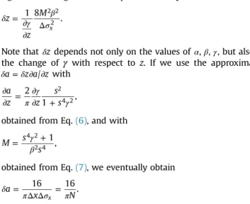
Note thatδzdepends not only on the values of α β γ, , , but also on the change of

γ

with respect to z. If we use the approximation

δa=δz a z∂ /∂ with π γ γ ∂ ∂ = ∂ ∂ + ( ) a z z s s 2 1 , 20 2 4 2

obtained from Eq.(6), and with

γ β = + ( ) M s s 1 , 21 4 2 2 4

obtained from Eq.(7), we eventually obtain

δ π σ π = Δ Δ = ( ) a x N 16 16 . 22 x

Notice that whileδzdepends on z, the value of δa does not depend on z nor any of the system parameters. It is a constant for given signal space–frequency extents. Thus the spherical reference sur-faces should be spaced equally with respect to the FRT order, rather than with respect to the distance. This is a generalization to QPSs, of the result we derived for Fresnel diffraction in[44], where we refer the reader for further discussion.

5. Discussion and conclusion

The non-uniform grid of samples points we have proposed has two constituents: the curved reference surfaces and the separation of samples on them. The parameters a, M, R deﬁne the curved surface structure, which mirrors the physical structure of the QPS. The parameters Δxand Δσxdeﬁnes s and δa, which mirrors the

information content of the set of signals. The special value

σ

= Δ Δ

s x/ x matches the structure of the grid to the natural

pro-pensity of the signal to diffract, as determined by its space and frequency extent[37].Fig. 2shows the natural sampling grid for an example system consisting of multiple lenses and sections of free space.

In conclusion, we derived a natural sampling grid that mirrors the fundamental structure of optical propagation through quad-ratic-phase systems. This grid is optimal in that it allows non-re-dundant representation of signals with the fewest number of samples and allows their efﬁcient fast processing. The longitudinal spacing is uniform with respect to the FRT order.

References

[1]H.M. Ozaktas, Z. Zalevsky, M.A. Kutay, The Fractional Fourier Transform with

Applications in Optics and Signal Processing, Wiley, NY, 2001.

[2]H. Liu, Y. Lu, J. Xia, X. Pu, L. Zhang, Propagation of an Airy-Gaussian beam

passing through the ABCD optical system with a rectangular aperture, Opt.

Commun. 355 (2015) 438–444.

[3]H. Liu, et al., Research on propagation properties of controllable hollow

ﬂat-topped beams in turbulent atmosphere based on ABCD matrix, Opt. Commun.

334 (2015) 133–140.

[4]X. Liu, D. Zhao, Fractional Fourier transforms of electromagnetic rectangular

Gaussian Schell model beams, Opt. Commun. (2015) 181–187.

[5]K.B. Wolf, Integral Transforms in Science and Engineering, Plenum, NY, 1979.

[6]J.J. Healy, M.A. Kutay, H.M. Ozaktas, J.T. Sheridan, Linear Canonical Transforms

—Theory and Applications, Springer, NY, 2016.

[7]K.B. Wolf, Development of linear canonical transforms: a historical sketch, in:

J.J. Healy, et al., (Eds.), Linear Canonical Transforms, Springer, NY, 2016,

pp. 3–28.

[8]K.B. Wolf, Canonical transforms I: complex linear transforms, J. Math. Phys. 15

(1974) 1295–1301.

0

5

10

15

20

25

30 -4

-3

-2

-1

0

1

2

3

4

0

5

10

15

20

25

30

0

1

2

3

4 x/s

FRT order

z/s

f

1

f

2

f

3

f

4

f

5

f

6

(a)

(b)

Fig. 2. (a) Natural sampling grid and (b) FRT order parameter for an optical system. The focal lengths are f1=10 /3s , f2=8 /3s , f3=10 /3s , f4=14 /3s , f5=10 /3s ,

=

f6 20 /3s , and λ = s/6. The axes are also normalized with the optimal scale

parameters= Δ Δx/ σx. For better visualization, the longitudinal spacing has been chosen 4 times denser than given by Eq.(22).

(5)

[9]T. Alieva, M.J. Bastiaans, Alternative representation of the linear canonical

integral transform, Opt. Lett. 30 (2005) 3302–3304.

[10]T. Alieva, M.J. Bastiaans, Properties of the linear canonical integral

transfor-mation, J. Opt. Soc. Am. A 24 (2007) 3658–3665.

[11]K.B. Wolf, A top-down account of linear canonical transforms, SIGMA 8 (2012)

033.

[12]L. Onural, Sampling of the diffractionﬁeld, Appl. Opt. 39 (2000) 5929–5935.

[13]A. Stern, Sampling of linear canonical transformed signals, Signal Process. 86

(2006) 1421–1425.

[14]J.J. Healy, B.M. Hennelly, J.T. Sheridan, Additional sampling criterion for the

linear canonical transform, Opt. Lett. 33 (2008) 2599–2601.

[15]J. Healy, J. Sheridan, Sampling and discretization of the linear canonical

transform, Signal Process. 89 (2009) 641–648.

[16]J. Shi, X. Liu, X. Sha, N. Zhang, Sampling and reconstruction of signals in

function spaces associated with the linear canonical transform, IEEE Trans.

Signal Process. 1 (2012) 6041–6047.

[17]D. Wei, Q. Ran, Y. Li, Sampling of bandlimited signals in the linear canonical

transform domain, Signal Image Video Process. 7 (2013) 553–558.

[18]J.J. Healy, H.M. Ozaktas, Sampling and discrete linear canonical transforms, in:

J.J. Healy, et al., (Eds.), Linear Canonical Transforms, Springer, NY, 2016,

pp. 241–256.

[19]S. Xu, Y. Chai, Y. Hu, C. Jiang, Y. Li, Reconstruction of digital spectrum from

periodic nonuniformly sampled signals in offset linear canonical transform

domain, Opt. Commun. 348 (2015) 59–65.

[20]Y.-H. Kim, G.H. Kim, H. Ryu, H.-Y. Chu, C.-S. Hwang, Exact light propagation

between rotated planes using non-uniform sampling and angular spectrum

method, Opt. Commun. 344 (2015) 1–6.

[21]D. Mendlovic, Z. Zalevsky, N. Konforti, Computation considerations and fast

algorithms for calculating the diffraction integral, J. Mod. Opt. 44 (1997)

407–414.

[22]D. Mas, J. Garcia, C. Ferreira, L.M. Bernardo, F. Marinho, Fast algorithms for

free-space diffraction patterns calculation, Opt. Commun. 164 (1999) 233–245.

[23]B.M. Hennelly, J.T. Sheridan, Generalizing, optimizing, and inventing

numer-ical algorithms for the fractional Fourier, Fresnel, and linear canonnumer-ical

trans-forms, J. Opt. Soc. Am. A 22 (2005) 917–927.

[24]B.M. Hennelly, J.T. Sheridan, Fast numerical algorithm for the linear canonical

transform, J. Opt. Soc. Am. A 22 (2005) 928–937.

[25]J. Healy, J.T. Sheridan, Fast linear canonical transforms, J. Opt. Soc. Am. A 27

(2010) 21–30.

[26]J. Healy, J.T. Sheridan, Reevaluation of the direct method of calculating Fresnel

and other linear canonical transforms, Opt. Lett. 35 (2010) 947–949.

[27]H.M. Ozaktas, B. Barshan, D. Mendlovic, L. Onural, Convolution,ﬁltering, and

multiplexing in fractional Fourier domains and their relation to chirp and

wavelet transforms, J. Opt. Soc. Am. A 11 (1994) 547–559.

[28] H.M. Ozaktas, D. Mendlovic, Fractional Fourier optics, J. Opt. Soc. Am. A 12

(1995) 743–751.

[29] H.M. Ozaktas, M.F. Erden, Relationships among ray optical, Gaussian beam,

and fractional Fourier transform descriptions ofﬁrst-order optical systems,

Opt. Commun. 143 (1997) 75–86.

[30] H.M. Ozaktas, A. Koc, I. Sari, M.A. Kutay, Efﬁcient computation of

quadratic-phase integrals in optics, Opt. Lett. 31 (2006) 35–37.

[31]A. Koc, H.M. Ozaktas, C. Candan, M.A. Kutay, Digital computation of linear

canonical transforms, IEEE Trans. Signal Process. 56 (2008) 2383–2394.

[32] A. Koc, H.M. Ozaktas, F.S. Oktem, Fast algorithms for digital computation of

linear canonical transforms, in: J.J. Healy, et al., (Eds.), Linear Canonical

Transforms, Springer, NY, 2016, pp. 293–327.

[33] M.J. Bastiaans, Wigner distribution function and its application toﬁrst-order

optics, J. Opt. Soc. Am. 69 (1979) 1710–1716.

[34] M.J. Bastiaans, Applications of the Wigner distribution function in optics, in:

W. Mecklenbrauker (Ed.), The Wigner Distribution: Theory and Applications in

Signal Processing, Elsevier, Amsterdam, 1997, pp. 375–426.

[35] M.J. Bastiaans, T. Alieva, The linear canonical transformation: deﬁnition and

properties, in: J.J. Healy, et al., (Eds.), Linear Canonical Transforms, Springer,

NY, 2016, pp. 29–80.

[36] T. Alieva, J.A. Rodrigo, A. Camara, M.J. Bastiaans, The linear canonical

trans-formations in classical optics, in: J.J. Healy, et al., (Eds.), Linear Canonical

Transforms, Springer, NY, 2016, pp. 113–178.

[37]H.M. Ozaktas, S.O. Arik, T. Coskun, Fundamental structure of Fresnel

diffrac-tion: natural sampling grid and the fractional Fourier transform, Opt. Lett. 36

(2011) 2524–2526.

[38] H.M. Ozaktas, O. Arikan, M.A. Kutay, G. Bozdagi, Digital computation of the

fractional Fourier transform, IEEE Trans. Signal Process. 44 (1996) 2141–2150.

[39] C. Candan, M.A. Kutay, H.M. Ozaktas, The discrete fractional Fourier transform,

IEEE Trans. Signal Process. 48 (2000) 1329–1337.

[40] X. Yang, Q. Tan, X. Wei, Y. Xiang, Y. Yan, G. Jin, Improved fast

fractional-Fourier-transform algorithm, J. Opt. Soc. Am. A 21 (2004) 1677–1681.

[41] F.S. Oktem, H. M. Ozaktas, Exact relation between continuous and discrete linear canonical transforms. IEEE Signal Process. Lett. 16 (2009) 727–730.

[42] F.S. Oktem, H.M. Ozaktas, Equivalence of linear canonical transform domains

to fractional Fourier domains and the bicanonical width product: a general-ization of the space–bandwidth product, J. Opt. Soc. Am. A 27 (2010)

1885–1895.

[43] F.S. Oktem, H.M. Ozaktas, Linear canonical domains and degrees of freedom of

signals and systems, in: J.J. Healy, et al., (Eds.), Linear Canonical Transforms,

Springer, NY, 2016, pp. 197–239.

[44]H.M. Ozaktas, S.O. Arik, T. Coskun, Fundamental structure of Fresnel

diffrac-tion: longitudinal uniformity with respect to fractional Fourier order, Opt. Lett.