A Bayesian approach to developing a strategic early
warning system for the French milk market
Christophe Bissona* and Furkan Gurpinarb
aKadir Has University, MIS department, Istanbul, Turkey
bBogazici University, Computer engineering department, Istanbul, Turkey
*Corresponding authors: [email protected] and [email protected]
Received 11 July 2017; accepted 27 October 2017
ABSTRACTA new approach is provided in our paper for creating a strategic early warning
system allowing the estimation of the future state of the milk market as scenarios. This is in line with the recent call from the EU commission for tools that help to better address such a highly volatile market. We applied different multivariate time series regression and Bayesian networks on a pre-determined map of relations between macro-economic indicators. The evaluation of our findings with root mean square error (RMSE) performance score enhances the robustness of the prediction model constructed. Our model could be used by competitive intelligence teams to obtain sharper scenarios, leading companies and public organisations to better anticipate market changes and make more robust decisions.
KEYWORDS Bayesian networks, competitive intelligence, forecasting, milk market, strategic
early warning system
1. INTRODUCTION
As globalisation, deregulation and the Big Data phenomenon (Bendler et al., 2014) are rendering our economy gradually more complex and uncertain, the interest in competitive intelligence (CI) is growing (Bisson, 2014; Hugues, 2017). Calof and Skinner (1998, p.38) define CI as “the art and science of preparing companies for the future by way of a systematic knowledge management process. It is creating knowledge from openly available information by use of a systematic process involving planning, collection, analysis, communication and management, which results in decision-maker action.”
However, Day and Schoemaker (2008) report that only 23% of CEOs use scanning, which is the upstream part of CI allowing the transfer of information from the environment to the organisation (see for example Bisson, 2013). By using scanning, managers detect most of the time weak signals (thereby
allowing to anticipate) through using their intuition (Cahen, 2010) and too often decisions are made on the basis of heuristics (Bisson et al., 2012). Therefore, in order to address challenges such as Big Data, highly volatile and uncertain environments, an era where anticipation is more important and more difficult than ever, “traditional” CI systems based on scanning appear to be limited (Accenture, 2013; Gilad, 2008). When trying to overcome these limitations and strengthen strategic planning and governance, the importance of strategic early warning systems (SEWS) has been raised (Fuld, 2010). SEWS can help decision-makers anticipate market changes, and allow organisations to have a strategy that fits the market reality and avoid industry dissonance. SEWS integrate scenario techniques which aim to “create alternative ‘pictures’ of the future and to challenge mental models” (Schwarz, 2005). The general framework of SEWS (Bisson, 2013; Gilad, 2008) for a market is: 1) define the scope, i.e.
Vol. 7, No. 3 (2017) pp. 25-34
the time frame, analysis to be done and participants; 2) determine the drivers of change; 3) generate scenarios; 4) explore strategic implications, options and decisions; and 5) implement the system by watching the drivers of change (through scanning), which could lead to the appearance of a pre-determined scenario, then launch an alert to anticipate either a threat or opportunity. SEWS requires updates to maintain its performances as inputs might change with time (Bisson et al., 2012). These updates regarding variables as well as other data/information must be provided by the competitive intelligence team. Our research focuses on the first three steps of the framework as we do not intend to implement it here. Although several qualitative methods of SEWS were developed which demonstrated their importance for governance (Gilad, 2003), there is room for improvements for SEWS based on quantitative methods (Fuld, 2010). Thus, we aim to address this scientific gap by applying for the first time different multivariate time series regressions and Bayesian networks following the three first steps of the general frame of SEWS to predict the impacting scenario(s) that would help to be better prepared for the future. For our experiment, we chose the milk sector in France in line with the call from the EU Commission (European Commission, 2010) for more robust tools to better predict the milk price and anticipate changes in this market. Indeed, the milk price is highly volatile. For instance, French farmers’ incomes can vary by over one third from one year to the next (Momagri, 2012). For example, a 1% or 2% discrepancy between supply and demand can trigger a variation of 50% to 100% change in income (Momagri, 2012). Yet, the European Union’s milk market is currently in crisis as the new Common Agricultural Policy, which went into effect in 2015, ended quotas for milk (Robert, 2015). Moreover, quotas will eventually end for other products as well (e.g. sugar in 2017).
The remainder of our paper is organised as follows: we first present the necessary theoretical background and provide an outline of the approaches used in the quantitative analysis of time series data. Next, we build the Bayesian model, apply it to our data, and we discuss the results obtained through Bayesian analysis. We conclude with comments on limitations and future research to be undertaken.
2. THEORETICAL BACKGROUND
2.1 Strategic Early Warning Systems
Although the development of SEWS is common among international companies, such as Shell (Gilad, 2003), the experiments and their details are rarely disclosed. Indeed, SEWS are central to governance, and their implementation can result in a competitive advantage synonymous to market share and profit increases (Bisson, 2013). SEWS can help to anticipate rather than react, and to detect strategic opportunities and risks (Gilad, 2003), reduce cognitive bias and intuition in the decision process, and allow for more effective contingency plans. Several types of SEWS have already been used, particularly in industry. SEWS are nowadays deemed to be compulsory for private organisations to survive and/or thrive (Fuld, 2010; Gilad, 2008). It can be argued that public organisations are also facing growing international competition, compelling them to most efficiently utilise tax funds. As a result, public organisations would benefit from implementing SEWS as well (Bisson et al., 2012) as demonstrated by the steel sector in the North American region of Pittsburgh (2008). Companies were closing one after another in 2008 (e.g. Seagate), due to the worst financial and economic crisis since 1929, and the sharp decline of the American automotive industry:
“the Steel Valley Authority (SVA) is an inter-municipal economic development agency incorporated by the City of Pittsburgh and eleven riverfront municipalities all within the Mon River region. The SVA has been managing industrial retention for the Commonwealth of Pennsylvania. The Authority, through a Strategic Early Warning Network (SEWN), has made significant contributions to the retention and revival of industrial enterprises, has saved and created nearly 8,000 jobs, and has impacted many more workers and communities indirectly. The SEWN Network has saved companies from Pittsburgh to Erie to Altoona, and has become a model state and nation-wide” (www.steelvalley.org).
Thus, a SEWS that is well developed and implemented can help private and public organisations succeed by allowing them to make better and faster strategic decisions in comparison to their competitors.
2.2 Time Series Forecasting
Financial time-series forecasting is considered to be one of the most difficult challenges of modern time-series forecasting. As explained by Abu-Mostafa and Atiya (1996), financial time-series data is usually noisy, non-stationary and deterministically chaotic. The term “noise” here actually represents the unavailability of data to capture the complex and non-linear relationships between market variables from past data. The non-stationary nature of data arises from the fact that the structure of relations between variables tends to change over time. The data is said to be chaotic because it usually behaves randomly in the short-term. However, under the assumption that there is a deterministic component in the long-term financial time-series data, we proceed to analyse and build a forecasting system, where the parameters are learned from the past data. The accuracy of time-series forecasting methods plays a crucial role in the economic and social benefits of competitive intelligence systems (Bisson, 2013). For building accurate forecasting systems, there are two main methodologies employed by researchers, namely, neural networks and support vector machines. Each of these methodologies has advantages and weaknesses, as explained below. The area of time-series forecasting is influenced by linear models such as autoregressive integrated moving average (ARIMA) and non-linear models such as the threshold autoregressive model, the bilinear model and the autoregressive heteroscedastic (ARCH) models (Engle, 1982). The linear ARIMA model, however, is clearly shown to be too weak to adopt in real-life scenarios (De Gooijer and Hyndman, 2006). Given that the traditional statistical forecasting methods lack the power of explaining the underlying structure, attention has been drawn to machine learning models, especially in the last two decades (Ahmed et al., 2010). Machine learning models are also called “data-driven”, or “black-box” models due to their nonparametric and nonlinear operation, which only requires the past data to learn the structure, and therefore perform future forecasting. For instance, artificial neural networks (ANNs) are shown to outperform their traditional opponents (such as linear regression) in the task of market forecasting (Lapedes and Farber, 1987; Werbos, 1988). Following ANNs, other machine learning models such as decision trees, nearest-neighbour regression and
support vector machines emerged for the task of future value forecasting (Alpaydin, 2010). Support vector machines are still widely used for classification and pattern recognition tasks, and they are shown to be a desirable alternative for classical learning methods for the task of time-series forecasting (Muller et al., 1997).
Statistical methods to analyse the structure and/or predict the future of the milk market have been implemented using a variety of methods in the previous works in the field.
Reed (1992) studied the structure of the market by optimising the parameters of different equations that are used to estimate the supply response from changes in demand and producer expectations. Another work by Saravanakumar and Jain (2009) proposes an econometric approach for determining the price of milk based on other variables of the market such as technology and input costs, by analysing the individual households of a local market.
Other research addresses the issue of better prediction for the milk market by using statistical learning methods. One example was done regarding the estimation of the entry and exit conditions to the milk market, based on quota and other policies regarding this market, by using the discrete variable of farm size in relation to other variables in a Markov chain analysis (Rahelizatovo and Gillespie, 1999). Markov chains are also employed in a recent work that studies the effect of trade quotas on milk, analysing the dairy sectors of Germany and Netherlands, again using categorical variables such as discretized milk production and firm size (Huettel and Jongeneel, 2008).
More than a decade ago, a research project funded by the European Commission resulted in the development of an economic model called Common Agricultural Policy Regional Impact (CAPRI), and aimed to deal with the complexity induced by the CAP reform in 1992 (Heckelei and Britz, 2000). A study based on CAPRI analysed the effect of removing milk quotas, and it obtained a prediction that the milk price would drop with respect to a reference scenario (Jansson and Britz, 2002). Another framework developed by the Food and Agricultural Policy Research Institute (FAPRI) examined and projected several variables related to agricultural markets. A study that utilised this framework to analyse the effect of removing milk quotas in the industry of the UK and the EU predicted a significant fall in milk
prices, as well as a recess in the expansion of milk production by 2016 (Patton et al., 2008).
2.3 Bayesian Networks
Bayesian networks are data structures that represent the relations between multiple parameters of a system. Bayesian networks, sometimes termed belief networks, causal networks or influence diagrams, are probability distributions factorised over a Directed Acyclic Graph (DAG). Although Bayesian networks were first introduced in the literature by Wright in 1921 to analyse the failures in crops, they are still widely used in dealing with uncertainty in knowledge based systems. Bayesian networks, as structure learning tools, are usually constructed with directed acyclic graphs where the leaf nodes are the observed variables and the lower-order nodes are the hidden (or cause) variables. Most of the time, the set of relations between the variables are given a priori. An example by Kiiveri, et al. (1984) analyses causal relations using a probability distribution factorised over a DAG. There are also variants of Bayesian networks to analyse dynamic systems such as
Hidden Markov Models (HMMs) (Durbin, 1998) and Dynamic Bayesian networks, as introduced by Murphy (2002).
Although we analyse a more complicated graph structure representing the relations of the major variables of our market, we also construct a DAG in order to represent a subset of variables, which have available time series data, by establishing the strength of relations using an expert evaluation, and we further investigate the data using this Bayesian network to get future value estimations, as described in Section 3.3.
3. METHODOLOGY
In this section, we apply Bayesian analysis in order to estimate and evaluate future scenarios for the milk market. Next we discretise the data and use the K-means clustering algorithm to classify the data in terms of amounts of change. This is followed by obtaining the prior probabilities needed to construct the Bayesian model. Finally, we evaluate the performance of our forecasting system and measure the probability for each scenario. To establish a broader understanding, we present our work in
Figure 1 System pipeline.
the form of a work flow diagram, as shown in Figure 1.
3.1 Data
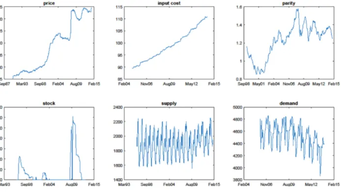
A questionnaire was first sent to a French milk expert (we were asked to keep his/her name confidential) to obtain all the drivers of change of the milk price which are macro-economic indicators. Thereafter, we started the quantitative analysis by collecting time series data for various price change drivers related to milk, which are world milk demand and production, the consumer price index for milk-related products, livestock and input costs (e.g. energy). We collected time series data for the period from January 1990 to February 2015, and normalised each time series vector by mapping its values between 0 and 1. Annotating the time t = 0 at the beginning of our observations, we have T = 319 time points where observations are recorded (see Figure 2). The time series data can be found at the website of INSEE (the French Public Official Statistic Organisation), an example data link is in the National Institute of Statistics and Economic Studies (2015). We also visualised the data and the autocorrelation function in Figures 3 and Figure 4, respectively.
Since the time series data for various indicators mentioned above came from different sources, some of them were measured in different units of time, such as monthly, quarterly and yearly. Therefore, to establish a consistent data set, we used linear interpolation and extrapolation to convert all the time series to monthly-observed variables. In order to impute the missing samples, we used least-squares approximation from applicable input variables, and thereby obtained the best linear unbiased estimation for the missing samples.
Figure 3 Reconstruction with different algorithms. KM: K-Means clustering, EM: expectation maximization.
3.2 Clustering
Next, we simplified the learning problem by converting the time series signals to discrete classes, then any given signal x is transformed to f(x)=𝑥". In the new form 𝑥", every element
𝑥#$ could have a value between 1 and V , where
V is the number of states. So, intuitively, the values of xd represent changes in the data (1:
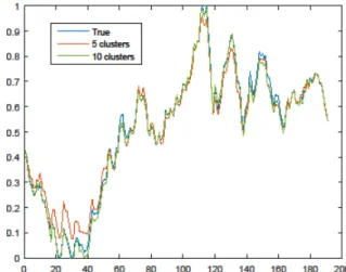
Big drop, 2: Smaller drop , ... V: Big rise). In Figure 4, we show that a higher number of cluster centres reduce the reconstruction error, however this means increasing the complexity of the classification system.
Therefore, to avoid overfitting and to be consistent with the 5-point Likert scale, we chose to set V =5 in our experiments. In order to find a reasonable set of changes, we used a K-means clustering algorithm which performs vector quantisation by finding optimal sets of clusters, and assigned each member of the vector to a cluster centre (MacQueen, 1967). We used the VL Feat library (Vedaldi et al., 2008) for the parallelised K-means implementation, which uses Lloyd’s algorithm (Lloyd, 1982) and L2 distance measure for optimisation. We started with a random initialization, repeated the clustering 10 times and chose the solution that gives the minimum energy. We found that K-means clustering provided better classification and forecasting accuracy than expectation maximization clustering.
In our application, we converted the signal to a format 𝑥& where this represents changes in
the data such that: 𝑥&$ = xi − 𝑥$ −1. We applied
clustering on this change vector 𝑥& , to find the
V most observed change values in the samples, and assigning each sample to one of the V cluster centers, we obtained the discrete vector 𝑥" as defined above.
Figure 4 Reconstruction with K-means algorithm and different number of clusters. KM: K-Means clustering, EM: expectation maximization.
3.3 Bayesian Analysis
Since our aim is to estimate the future values of dependent variables, we first needed to obtain prior probabilities to feed our Bayesian decision system. To this end, we used two different probability definitions, which can then be combined in a single set of matrices. Two different probability estimations are explained below. We started by finding the probability distributions of single variables over different time lags. In other words, we constructed probability distribution function (PDF) tables to establish the prior probability of observing variable i having the value k1 ∈ [1: V] when observed that it has the value k2 ∈ [1: V], on time (t − lag). Thus, we established a seasonal model where we have an estimation of probabilities of observing a single variable.
After normalisation, this yields a (VxV) PDF table T. Where T(,*,$ = p(x(\x(-.), in other words
the probability of observing x = j when we know that x = i [lag] periods before. Similar to the intra-variable approach, we construct prior probabilities which represent the effect of indicator variables on the dependent variables over different time lags, more formally p(𝑦0- |
𝑥.,(0-.), 𝑥3,(0-.), . . . , 𝑥45,(0-.)). Finally, we
obtained a set of V−by−V probability distribution matrices from the collected set of data. For the representation of PDFs, assuming that each variable depends on each other (a complete graph), we have a data structure of size 𝑁3by𝑉3 where N is the number of variables in
the model, and V is the number of classes. We compute the prior probabilities as described above, and use the posteriors to forecast the time series vectors and evaluate scenarios, which will be described next.
Having collected all the data and the prior probability distributions, we used our system for simulation, to determine the probability of a scenario happening 𝑇9 time periods after the
last observation. Therefore in our case, a scenario S is simply represented as an N by 1 vector where each member 𝑆𝑖 represents the numerical value of variable i, at the time period designated by T +𝑇9. Since we cannot measure
the accuracy of our system’s prediction with a large 𝑇9 value, we make validation tests with
forward chaining, as we explain next.
3.4 Performance Evaluation
In order to measure the accuracy of our forecasting system, we ran validation tests using the forward chaining strategy, which
means for each data point, we use the previous observations to construct our model, and measure the out of sample RMSE of the prediction on the point of interest. We use all five variables as explanatory variables and price of milk as the output. Averaging the results over all folds, the classification accuracy was 80.94% and the average RMSE was 0.0189. We also provide the performance with each input variable in Table 1. Here we keep the autoregressive component and compare the contributions of each explanatory variable. Therefore, the first row corresponds to estimation with only previous values of price.
Table 1 Forward chaining estimation accuracy of price with different input variables.
3.5 Scenario Assessment
Using the prior probabilities explained in Section 2, we used Bayes’ decision theorem to forecast the future values of our time-series signals. We represented our system’s state by N discrete time-series signals of length T, hence a T-by-N matrix. We fed this matrix into our simulation code and we obtained a new scenario of size (T +1) x N. The process is repeated until we reach time 𝑇9, and converting
the discrete signals back to the numerical values, we estimated the final values of variables. To analyse the probability of scenarios, we repeated this process many times, hence we obtained a probability distribution function for the scenario at time 𝑇9.
3.6 Simulation
Since our aim was to obtain a probability density function for the final values of the variables, we ran 1,000 simulations to forecast the values of the discrete time series vectors, and converting them back to continuous signals, we obtained one final value per parameter for each turn. Collecting all the final
values, we obtained a data distribution. By fitting a normal distribution on this data, we obtain a probability for a given scenario.
4. RESULTS AND DISCUSSION
To evaluate the accuracy of our framework, we ran some tests on different parts of the machine learning system, and we report performance scores in the following.
4.1 Signal Reconstruction Accuracy
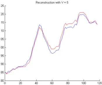
Here, we analyse the accuracy of our signal conversion system. As explained above, we convert our time series data into discrete values. Hence we need to reconstruct the signal back to a “continuous” time-series form, which inevitably causes information loss. Intuitively, increasing the number of cluster centres, k, in K-means clustering should decrease the reconstruction error. Here, we present a chart for a sample signal (namely the USD/EUR parity) which shows the relationship between the number of cluster centres and the Root Mean Square Error (RMSE) for signal reconstruction, in Figure 5 (an example signal reconstruction for 5 and 10 cluster centres are shown).
As expected, the reconstructed signal converged to the original one as the number of cluster centres increases. As is shown, there might still be room for improvement, but increasing the number of cluster centres is equivalent to increasing the complexity of the learning algorithm, and with a fixed amount of data, a high number of cluster centres might lead to over-learning. In order to evaluate the accuracy of our prediction system, we again used the RMSE error measure, with a performance test similar to a machine learning application. In this test, we used the parameter
τ ∈ [0, 1] which is the ratio of training set size to the data set size D. In other words, we used the first τD number of observations for the learning (see Section 3.3), and we ran a simulation for the remaining (1 − τ) D unobserved time periods, and thus constructed a scenario which is of size D. After obtaining a large (∼10>) number of scenarios, and taking
the mean of them, we estimated the signal 𝑆?
for the variable of interest. Since we already knew the original signal S, we represented our system’s performance with the Root Mean Square Error RMSE(S,𝑆?). Below in Table 2 are
some results for different variables and different values of τ.
Table 2 Forecast error vs. τ.
4.2 Scenario Probability Evaluation
Finally, we used our framework to estimate the probability of different scenarios relevant to the milk market. Two scenarios were given in terms of milk price, and another one about the milk demand in the European Union (Pole Economie & Prospective Normandie, 2014). We tested these scenarios by propagating the market’s state up to the year 2020, with the method explained in Section 3.6. The results for the 3 scenarios are shown in Table 3.
We tested our algorithm with different scenarios for the variables of price and demand. As expected, the likely scenario resulted in a high probability value, whereas
the probability of the pessimistic scenario (price decreases by 15 % scenario) resulted in a low probability value. However, the highest probability is for the optimistic scenario. Hence, we observe a difference between the results obtained with the prospective (or foresight) approach (which is purely qualitative and for the long term) and the approaches obtained with our simulation for SEWS.
Table 3 Scenario probabilities.
About the milk market, although prices are currently lower compared to before the end of quotas on the first of April 2015, our optimistic scenario might occur in 2020, as after a price drop the market will certainly concentrate and price might increase again.
A competitive intelligence team could use, feed and update this model by entering new variables, new inputs such as new prices and production levels among others and see the most probable scenarios in the coming months and years. Therefore, it would help organisations to be better prepared for the future and lead toward stronger decisions.
5. CONCLUSION
We applied for the first time different multivariate time series regression and Bayesian networks to predict the impacting scenarios which are the heart of SEWS. Our model could inspire competitive intelligence teams in order to seek more accuracy regarding scenarios, leading to better anticipate opportunities and/or threats, and to more robust decisions.
6. LIMITATIONS
Our work models both small and big changes, but to create better scenarios, we need more data for such complex relationships. Experts in the field together with competitive intelligence experts could make further searches to get a stronger understanding of the underlying procedures.
7. FURTHER WORK
Our regression is learned in one shot, so there are no iterations, and therefore there is no correction. Thus, by using machine learning algorithms, we could get automatic corrections and potentially proffer toward better accuracy of scenarios. As such, it could lead to better anticipation and decisions. Furthermore, this technology would help to process more data and dig into “Big Data”.
Understanding the strategic needs, guiding through data modelling and interpreting the results is where competitive intelligence specialists will add increasingly great value to companies and public organisations.
ACKNOWLEDGEMENTS
This work was supported by the Kadir Has University Research Grant [Grant Number 2014-BAP-07].
8. REFERENCES
Andaluz, D. J., & Sánchez J. (2006). Nanotecnología en España. http://www. madrimasd.
org/revista/revista34/tribuna/tribuna4.asp (Accessed: 05.02.2015)
Abu-Mostafa, Y. S., & Atiya, A. F. (1996). Introduction to financial forecasting. Applied
Intelligence, 6(3), 205–213.
Accenture (2014). Accenture and MIT Form Alliance for Advanced Analytics Solutions. Retrieved on 20-April-2015, from http://newsroom.accenture.com/news/accentu re-and-mit-form-alliance-for-advanced-analytics-solutions.htm.
Ahmed, N. K., Atiya, A. F., Gayar, N. E., & El-Shishiny, N. (2010). An empirical comparison of machine learning models for time series forecasting. Econometric Reviews, 29(5-6), 594–621.
Alpaydin, E (2010). Introduction to machine
learning. Cambridge, Massachusetts: The
MIT Press.
Bisson, C. (2013). Guide de gestion stratégique de
l’information pour les PME. Montmoreau:
Les2Encres.
Bisson, C. (2014). Exploring Competitive Intelligence Practices of French Local Public Agricultural Organisations. Journal of
Intelligence Studies in Business, 4(2), 5-29.
Bisson, C., Guibey, I., Laurent, R., & Dagron, P. (2012). Mise en place d’un Système de détection de Signaux Précoces pour une
Intelligence Collective de l’Agriculture applique aux filières de l’élevage bovin. Proceedings of the PSDR symposium, Clermont Ferrand, France.
Bendler, J., Wagner, S., Brandt, D.-V. T. & Neumann, D. (2014). Taming uncertainty in big data. Business & Information Systems
Engineering, 6(5), 279– 288.
Cahen, P. (2010). Signaux faibles, mode d'emploi. Paris: Eyrolles.
Calof, J.L. & Skinner, B. (1998). Competitive intelligence for government officers: a brave new World. Optimum, 28 (2), 38-42.
Day, G.S. & Schoemaker, P.J.H. (2008). Leadership –Are you a ‘‘vigilant leader’’? MIT
Sloan Management Review, 49, 43.
De Gooijer, J. G. & Hyndman, R. J. (2006). 25 years of time series forecasting. International
journal of forecasting, 22(3), 443–473.
Durbin, R., Eddy, S. R., Krogh, A.,& Mitchison, G. (1998). Biological sequence analysis: probabilistic models of proteins and nucleic acids. Cambridge: Cambridge university
press.
Engle, R. F. (1982) Autoregressive conditional heteroscedasticity with estimates of the variance of United Kingdom inflation.
Econometrica: Journal of the Econometric Society, 50(4), 987–1007.
European Commission (2010). Evolution of the market situation and the consequent conditions for smoothly phasing-out the milk quota system second soft landing report. Report from the commission to the European parliament and the council, Brussels.
Fuld, L., (2010). The Secret Language of
Competitive Intelligence: How to See Through & Stay Ahead of Business Disruptions,
Distortions, Rumors & Smoke
Screens. Indianapolis: Dog Ear Publishing.
Gilad, B. (2003). Early warning: using
competitive intelligence to anticipate market shifts, control risk, and create powerful strategies. New-York: Amacom.
Gilad, B. (2008). Business War games: How large,
small, and new companies can vastly improve their strategies and outmaneuver the competition. Pompton Plains: Career press.
Heckelei, T., & Britz, W. (2000). Concept and explorative application of an EU wide regional agricultural sector model (capri-project). In: Agricultural sector modeling and policy
information systems. Proceedings of the 65th EAAE Seminar (pp. 281–290), Bonn, Germany.
Huettel, S., & Jongeneel, R. (2008). Structural change in the dairy sectors of Germany and the Netherlands–a markov chain analysis. Proceedings of the 12th EAAE 395 Congress (pp. 26–29), Bonn, Germany.
Hugues, S. (2017). A new model for identifying emerging technologies. Journal of Intelligence
Studies in Business. 7(1), 76-86.
Jansson, T., & Britz, W. (2002). Experiences of using a quadratic programming model to simulate removal of milk quotas. Proceedings of the 10th EAAE-Conference, Ghent, Belgium.
Kiiveri, H., Speed, T. P., & Carlin, J. B. (1984). Recursive causal models. Journal of the
Australian Mathematical Society. 36(01), 30–
52.
Lapedes, A., & Farber, R. (1987). Nonlinear signal processing using neural networks: Prediction and system modeling. Technical report, Los Alamos National Laboratory, Los Alamos.
Lloyd, S. P. (1982). Least squares quantization in pcm. IEEE Transactions on Information
Theory, 28 (2), 129–137.
MacQueen, J. (1967). Some methods for classification and analysis of multivariate observations. Proceedings of the fifth Berkeley symposium on mathematical statistics and probability, Vol. 1 (pp. 281–297), California, USA.
Momagri (2012). Chiffres clés de l’agriculture.
Retrieved on 15-May-2016, from
http://www.momagri.org/FR/chiffres-cles-de-l-agriculture.http://www.momagri.org/FR/chiffr es-cles-de-l-agriculture.html
Muller, K.-R., Smola, A. J., Ratsch, G., Scholkopf, B. Kohlmorgen, J. & Vapnik, V. (1997). Predicting time series with support vector machines. In: Artificial Neural Networks. Proceedings of the ICANN’97 (pp. 999–1004), Springer.
Murphy, K. P.( 2002). Dynamic bayesian networks: representation, inference and learning. Ph.D. thesis, University of California, Berkeley.
National Institute of Statistics and Economic Studies (2015). Macro-economic database. Retrieved on 18-November-2015, from
http://www.bdm.insee.fr/bdm2/choixCriteres? codeGroupe=1466.
Patton, M., Binfield, J., Moss, J., Kostov, P., Zhang, L., Davis,J., & Westhoff, P. (2008). Impact of the abolition of EU milk quotas on agriculture in the UK Proceedings of the 107th EAAE Seminar, Sevilla, Spain.
Pole Economie & Prospective Normandie (2014). Quels élevages laitiers en Normandie 2020, Synthese.2. Retrieved on 12-November-2014, from http://www.chambre-agriculture-
27.fr/toutes-les-publications-
normandes/detail- publication/actualites/quels-elevages-laitiers-en-normandie-2020/
Rahelizatovo, N. C., & Gillespie, J. M. (1999). Dairy farm size, entry, and exit in a declining production region. Journal of Agricultural and
Applied Economics, 31(2), 333–347.
Reed, A. J. (1992). Expectations, demand shifts, and milk supply response. Journal of
Agricultural Economics Research, 44(1),
11-21.
Robert, A. (2015). Milk crisis drives wedge between France and Germany. Retrieved
15.September-2015, from:
https://www.euractiv.com/section/agriculture- food/news/milk-crisis-drives-wedge-between-france-and-germany/
Saravanakumar, V., & Jain, D. (2009). Evolving milk pricing model for agribusiness centres: an econometric approach. Agricultural
Economics Research Review, 22 (1), 155–160.
Schwarz, J. O. (2005). Pitfalls in implementing a strategic early warning system. Foresight, 7(4), 22–30.
Vedaldi, A., & Fulkerson, B. (2008). VLFeat: An open and portable library of computer vision algorithms. Retrieved 25.September-2016, from http://www.vlfeat.org/
Werbos, P. J. (1988). Generalization of back propagation with application to a recurrent gas market model. Neural Networks, 1(4), 339–356.
Wright, S. (1921). Correlation and causation.
Journal of agricultural research, 20(7), 557–
585.
View publication stats View publication stats