a thesis
submitted to the department of physics
and the institute of engineering and science
of bilkent university
in partial fulfillment of the requirements
for the degree of
master of science
By
Sinem Binicio˘glu C
¸ etiner
September, 2003
Prof. Dr. Igor O. Kulik (Supervisor)
I certify that I have read this thesis and that in my opinion it is fully adequate, in scope and in quality, as a thesis for the degree of Master of Science.
Assist. Prof. Ceyhun Bulutay
I certify that I have read this thesis and that in my opinion it is fully adequate, in scope and in quality, as a thesis for the degree of Master of Science.
Prof. Dr. Iossif V. Ostrovskii
Approved for the Institute of Engineering and Science:
Prof. Dr. Mehmet Baray
Director of the Institute of Engineering and Science
Sinem Binicio˘glu C¸ etiner M.S. in Physics
Supervisor: Prof. Dr. Igor O. Kulik September, 2003
Carbon nanotubes are one of the most important findings of physics in the recent years. They are of great interest because of their various electrical, and mechanical features. All the properties of the nanotubes are being investigated thoroughly.
In my thesis, two dimensional helical potential is introduced. The problem takes the type of Kronig-Penney model when Hamiltonian is separated into two parts. I will investigate the persistent currents in helical nanotubes. Persistent currents are due to the external vector potential. Vector potential was first in-troduced as a mathematical tool, later Aharonov and Bohm showed that vector potential has effect on charged particles even there is no magnetic field (i.e. field is confined into a solenoid).
Keywords: Carbon Nanotubes, Aharonov-Bohm Effect, Persistent Currents,
Kronig-Penney Model.
KARBON NANOT ¨
UPLERDE DEVAMLI AKIMLAR
Sinem Binicio˘glu C¸ etinerFizik, Y¨uksek Lisans
Tez Y¨oneticisi: Prof. Igor O. Kulik Eyl¨ul, 2003
Karbon nanot¨upler fizikte son yıllardaki en ¨onemli bulu¸slardan biridir. Kar-bon nanot¨upler, ¸sa¸sırtıcı elektriksel ve mekaniksel ¨ozellikleriyle de b¨uy¨uk ¨onem ta¸sımaktadırlar. B¨ut¨un ¨ozellikleri ara¸stırılmaktadır.
Bu tezde, iki boyutlu bir sarmal potansiyel du¸s¨un¨ulm¨u¸st¨ur. Hamilton denklemi iki par¸caya ayrıldıktan sonra problemin Kronig-Penney tipi oldugu g¨or¨ulmektedir. Bu tezde karbon nanot¨uplerdeki devamlıakımlar incelendi. Devamlıakımlar vekt¨or potansiyel sebebiyle olu¸smaktadır. Vekt¨or potansiyel ¨onceleri bir matematiksel ara¸c olarak kullanıldıysa da Aharonov ve Bohm potan-siyelin y¨ukl¨u par¸cacıklar ¨uzerindeki etkisini g¨ostermi¸stir, ortamda manyetik alan olmamasına ra˘gmen (Mesela manyetik alan selenoidin i¸cine hapsedilmi¸stir).
Anahtar s¨ozc¨ukler : Karbon Nanot¨upler, Aharonov-Bohm, Devamlı Akımlar,
Kronig-Penney Modeli.
Thanks to Prof. Dr. Igor O. Kulik for his guidance and help, thanks to my friends for their encouraging help, thanks to my family for their emotional and financial support throughout all my life, and also thanks to Ender, for he was always with me.
1 Introduction 1
1.1 Carbon Nanotubes . . . 1
1.2 Aharonov-Bohm Effect and Persistent Currents . . . 6
1.2.1 Aharonov-Bohm Resistance Oscillations in Multi-walled Carbon Nanotubes . . . 10
1.3 Kronig-Penney Model . . . 13
1.4 Organization of the Thesis . . . 15
2 Part I 16 2.1 Statement of the Problem . . . 16
2.2 Periodic boundary conditions: . . . 24
2.3 Summary: . . . 26
2.4 Density of states: . . . 27
3 Part II 31 3.1 Magnetic Field Parallel to the Cylinder Axis, ~Bα. . . 32
3.1.1 Periodic boundary conditions: . . . 35
3.1.2 Summary: . . . 35
3.1.3 Density of states: . . . 37
3.1.4 Persistent Currents: . . . 38
3.2 Additional Magnetic Field, Perpendicular to the Cylinder Axis, ~Bβ 40 3.2.1 Periodic boundary conditions: . . . 42
3.2.2 Summary: . . . 42
3.2.3 Density of states: . . . 43
3.2.4 Persistent Currents: . . . 45
4 Conclusions and Future Work 47 5 Appendix 49 5.1 ABC . . . 49
1.1 The Chiral Vector . . . 2 1.2 Types of CNT . . . 2 1.3 STM map of a wavefunction. The white lines represent the
hexag-onal atomic lattice, clearly demonstrating that the electronic wave-functions have a different periodicity than that of the atomic lat-tice. The wavefunction can be understood by considering the elec-tronic structure of a graphite sheet. . . 3 1.4 STM view of CNT . . . 4 1.5 Persistent Current in one dimesional metallic loop . . . 7 1.6 Illustration of Aharonov-Bohm effect in a ring geometry. (a)
Tra-jectories responsible for hc/e periodicity, (b) traTra-jectories of the pair of time-reversed states leading to hc/2e periodicity. . . . 10 1.7 Diagram of a MWNT, composed of a series coaxial cylinders. A
periodic magneto-resistance is expected to originate from quantum interference of back-scattered electron trajectories . . . 11
1.8 (Top left) In the standard Aharonov-Bohm effect the magnetic flux through the solenoid changes the relative phase of the electron waves in paths 1 and 2, there is an interference pattern forms on the screen. When the flux is changed, the interference pattern shifts on the screen. (Top right) Carbon nanotube is placed in a magnetic field parallel to the its axis. In the nanotube, there are two paths, clockwise and anticlockwise around the nanotube. These paths interefere and the shift in the interference pattern manifests itself as a change in the electrical resistance along the nanotube as a function of magnetic field (bottom). The magnetic field at the peaks can be related to the quantum of magnetic flux,
hc/2e, and the cross-section of the nanotube. . . . 12
1.9 periodic potential . . . 13
1.10 Shaded region indicates allowed energy bands. The band width is indicated by ∆E . . . . 14
1.11 The ”reduced zone representation” shows that the bands (i.e., the values of k) only range within the First Brillouin Zone (FBZ).The width of the First Brillouin Zone (FBZ) corresponds to the mag-nitude of the primitive reciprocal lattice vector. . . 14
2.1 Potential . . . 16
2.2 V(u), u dependent potential . . . 18
2.3 Kronig-Penney relation with positive g value . . . . 20
2.4 Kronig-Penney relation for negative g, when potential consists wells instead of barriers . . . 20
2.5 Energy-band diagram for g=0 . . . 21
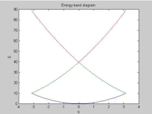
2.7 Energy-band diagram for g=2 . . . 22
2.8 Energy-band diagram for g=1 . . . 22
2.9 Energy-band diagram for g=-1 . . . 23
2.10 Energy-band diagram for g=-2 . . . 23
2.11 Energy-band diagram for g=-4 . . . 23
2.12 Density of States for g=0 . . . 27
2.13 Density of States for g=6 . . . 29
2.14 Density of States for g=4 . . . 29
2.15 Density of States for g=2 . . . 29
2.16 Density of States for g=-2 . . . 30
2.17 Density of States for g=-4 . . . 30
2.18 Density of States for g=-6 . . . 30
3.1 Cylindrical coordinates . . . 31 3.2 B~α . . . 32 3.3 g = 1, (cos γ)2 Φα Φ0 = 1 2 . . . 34 3.4 g = 1, (cos γ)2 Φα Φ0 = 1 3 . . . 34
3.5 b = L/M and a is the circumference of the cylinder . . . . 36
3.6 g=1, Φα = 4Φ0, with b = 1, a = √ 3. . . 37 3.7 Persistent current I1, found for electrons fill 3/4 of the first band . 39
3.8 B~β is the along the direction perpendicular to the torus axis, ~Aβ
is along the cylinder, ˆy axis. . . . 40 3.9 g = 1, (cos γ)2 Φα Φ0 = (cos γ) 2 Φβ Φ0 = 1 3, M = 10 . . . . 41 3.10 g=1, Φα = Φβ = 2Φ0, with b = 1, a = √ 2, M = 10. . . . 44 3.11 Persistent current I1, found for Φα = Φβ, electrons fill 3/4 of the
Introduction
As our information about the nature increased, the sizes we are interested de-creased. This is partly because of just curiosity, and partly to improve the tech-nology. Carbon nanotubes are one of the most important and interesting subjects of the nanotechnology. In this thesis, persistent currents in carbon nanotubes is investigated. In the introduction part of the thesis, a brief summary about car-bon nanotubes is given. Later, Aharonov- Bohm effect and persistent currents are discussed, and lastly Penney model is explained. We introduce Kronig-Penney type potential to our problem, since this potential is exactly solvable.
1.1
Carbon Nanotubes
The discovery of the carbon nanotubes was accidental, as it has been the same for some of the greatest findings of the physics. Carbon nanotubes are fullerene-related structures which consist of graphene cylinders closed at either end with caps containing pentagonal rings. They were discovered by Ijima [1] who was studying the material deposited on the cathode during the arc-evaporation synthesis of fullerenes [2]. During the experiment, he observed various closed graphitic structures including nanoparticles and nanotubes, of a type which had never previously been observed. CNT’s have very remarkable electronic and
Figure 1.1: The Chiral Vector
mechanical properties, also they can be considered as prototypes for a one-dimensional quantum wire [3].
Although Iijima’s first observations were of multi-wall nanotubes, he observed single-wall carbon nanotubes less than two years later, in 1993. Many studies have explored the structure of carbon nanotubes using high-resolution microscopy techniques. These experiments have confirmed that nanotubes are cylindrical structures based on the hexagonal lattice of carbon atoms that forms crystalline graphite. Three types of nanotubes are possible, called armchair, zigzag and chiral nanotubes, depending on how the two-dimensional graphene sheet is rolled, CNT is based on this sheet [4].
Figure 1.2: Types of CNT The chiral vector is defined on the hexagonal lattice as
Ch = nˆa1+ mˆa2,
where ˆa1 and ˆa2 are the unit vectors, and n and m are integers. The chiral angle,
θ, is measured relative to the direction defined by ˆa1. The diagram in the figure
1.1, has been constructed for (n, m) = (4, 2), and the unit cell of this nanotube is bounded by OAB0B. To form the nanotube, this cell is rolled up so that O
molecule, so the size of the nanotube can be as small as the size of a fullerene molecule [3, 4].
The properties of nanotubes are determined by their diameter and chiral angle, both of which depend on n and m. The diameter, dt, is the length of the chiral
vector multiplied by 4. At figure 1.2, (5, 5) is an armchair nanotube (top), (9, 0) is an zigzag nanotube (middle) and (10, 5) is an chiral nanotube.
Armchair nanotubes are formed when n = m and the chiral angle is 30. Zigzag nanotubes are formed when either n or m are zero and the chiral angle is 0. All other nanotubes, with chiral angles intermediate between 0 and 30, are chiral nanotubes.
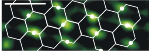
Figure 1.3: STM map of a wavefunction. The white lines represent the hexagonal atomic lattice, clearly demonstrating that the electronic wavefunctions have a different periodicity than that of the atomic lattice. The wavefunction can be understood by considering the electronic structure of a graphite sheet.
Since each unit cell of a nanotube contains a number of hexagons, each of which contains two carbon atoms, the unit cell of a nanotube contains many carbon atoms. If the unit cell of a nanotube is N times larger than that of a hexagon, the unit cell of the nanotube in reciprocal space is 1/N times smaller than that of a single hexagon [4].
In a scanning electron microscope, nanotubes can be imaged with atomic res-olution, and the chiral winding of the hexagons along the tube can be observed. The nanotube material looks like a mat of carbon ropes. The ropes are between 10 and 20 nm across and up to 100µm long. When examined in a transmission electron microscope, each rope is found to consist of a bundle of single-wall car-bon nanotubes aligned along a single direction. The STM can also be used to obtain spectroscopic information, i.e., to measure the electronic density of states of the nanotube. It has been found that nanotube spectra fall into two classes:
metallic and semiconducting . In particular, the size of the observed gaps are
in quantitative agreement with the calculations, by the experiments made with electron microscope [3].
Figure 1.4: STM view of CNT
The electronic properties of CNT’s are due to the quantum confinement of electrons normal to the nanotube axis. In the radial direction, electrons are con-fined by the monolayer thickness of the graphene sheet. Around the circumference of the nanotube, periodic boundary conditions come into play. For example, if a zigzag or armchair nanotube has 10 hexagons around its circumference, the 11th
hexagonal will coincide with the first. Going around the cylinder once introduces a phase difference of 2π.
Because of this quantum confinement, electrons can only propagate along the nanotube axis, and so their wavevectors point in this direction. The resulting number of one-dimensional conduction and valence bands effectively depends on the standing waves that are set up around the circumference of the nanotube. These simple ideas can be used to calculate the dispersion relations of the one-dimensional bands, from the well known dispersion relation in a graphene sheet. In general, an (n, m) carbon nanotube will be metallic when n − m = 3q, where q is an integer. All armchair nanotubes are metallic, as are one-third of all possible zigzag nanotubes.
Although the choice of n and m determines whether the nanotube is metallic or semiconducting, the chemical bonding between the carbon atoms is exactly the same in both cases. This surprising result is due to the very special electronic structure of a two-dimensional graphene sheet, which is a semiconductor with a zero band gap. In this case, the top of the valence band has the same energy as the bottom of the conduction band, and this energy equals the Fermi energy for one special wavevector, the so-called K-point of the two-dimensional Brillouin zone (i.e. the corner point of the hexagonal unit cell in reciprocal space). Theory
shows that a nanotube becomes metallic when one of the few allowed wavevectors in the circumferential direction passes through this K-point.
As the nanotube diameter increases, more wavevectors are allowed in the circumferential direction. Since the band gap in semiconducting nanotubes is inversely proportional to the tube diameter, the band gap approaches zero at large diameters, just as for a graphene sheet. At a nanotube diameter of about 3 nm, the band gap becomes comparable to thermal energies at room temperature.
1.2
Aharonov-Bohm Effect and Persistent
Cur-rents
Aharonov-Bohm effect is one of the most fundamental phenomena in quantum physics. In the Aharonov-Bohm effect a beam of quantum particles, such as electrons, is split into two partial beams that pass on either side of a region containing a magnetic field, and these partial beams are then recombined to form an interference pattern. The interference pattern can be altered by changing the magnetic field - even though the electrons do not come into contact with the magnetic field.
The observation of the interference pattern demonstrates that a single electron does not choose a particular path but behaves as an extended wave and follows both paths simultaneously. The interference pattern shifts as the magnetic field changes, returning to the original pattern when the magnetic flux has changed by the quantum of magnetic flux, φ0 = hc/e.
The Aharonov-Bohm effect is particularly interesting because it depends on the electromagnetic vector potential, ~A, which is related to the magnetic field,
~
B, through the equation, ~B = ∇ × ~A. Originally it was thought that the vector
potential, ~A, did not have a physical meaning (various quantities can be added
to ~A without changing the value of the physical observable, ~B). Scalar potential φ and vector potential ~A were first introduced as mathematical tools for
cal-culation concerning electromagnetic fields. However, the theoretical prediction of the Aharonov-Bohm effect, and its subsequent confirmation in experiments, showed that this is not the case. In quantum theory these potentials appear in the Schr¨odinger equation explicitly and therefore they affect all physical quanti-ties directly. This effect has purely quantum mechanical origin because it comes from the interference phenomenon.
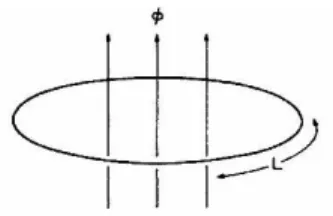
Persistent (non-decaying) currents were first observed at superconductors. Ex-istence of non-decaying current in normal-metal rings (where mean free path Lφ
predicted by Kulik in 1970 [6]. Later B¨uttiker, Imry, and Landauer proposed the persistent current in the normal one-dimensional disordered ring [7]. In 1990’s, experimental works confirmed the existence of persistent current in mesoscopic rings [11, 12]. This current arises due to to the boundary conditions imposed on the wave function by the doubly connected nature of the loop [9]. As a conse-quence of the boundary conditions, all physical properties of the ring are periodic in the magnetic flux φ with a period φ0 = hc/e.
Scattering mechanisms result in decreasing, but not diminishing, of the persis-tent current. It is believed that inelastic, i.e. electron-phonon interaction, should be small to make the electronic states in the ring long-lived (phase conserving). In the literature, the effects of the electron-phonon interaction were studied in the mesoscopic Aharonov-Bohm rings in metallic and semiconducting links [10].
Figure 1.5: Persistent Current in one dimesional metallic loop
Below calculations show persistent currents in one-dimensional metallic ring: Magnetic field ~B parallel to the ring axis, so ~A = Aˆx. Direction of ˆx is along
the ring circumference, and φ = x/R. Hamiltonian without ~B: −¯h2
2mR2
∂2
∂φ2ψ = εψ
Solution of this equation:
ψ = c · eikφ
By using boundary condition ψ(0) = ψ(2π) and normalization:
ψ = √1 Le
εn=
n2¯h2
2mR2
εn is the energy without magnetic field. Calculations with ~B:
−¯h2 2mR2( ∂ ∂φ− ieAL hc ) 2ψ = εψ A · L = Φ and hc
e = Φ0. Where Φ is the flux and Φ0 is the flux quantum.
Solution of the above equation is ψ = c · ek0, k0
= −eAL hc ±R¯h
√
2mε.
(only + term is used since there is no potential barrier or well). By using periodic boundary condition, and normalization, we get the same answer for wavefunction: ψ = √1 Le inφ For energy: εn= ¯h2 2mR2(n − Φ Φ0 )2 Persistent current In: In= −c ∂εn ∂Φ = ¯h2 mR2Φ 0 (n − Φ Φ0 )
When the ring is interrupted by a potential, V = V0δ(x) = V0δ(R · φ), the
Hamiltonian becomes: −¯h2 2mR2( ∂ ∂φ− ieAL hc ) 2ψ + V 0δ(R · φ)ψ = εψ
For solution at 0 < φ < 2π, we get same k0 value as above.
k0 = −eAL hc ± R ¯h √ 2mε
ψ = c1ei(k+Φ/Φ0)+ c2e−i(k−Φ/Φ0)
By using the boundary condition
ψ(0) = ψ(2π)
and the relation obtained by integrating the Hamiltonian
−¯h2
2mR2 ³
ψ0(2π) − ψ0(0)´+ V ψ(0) = 0 we can get the relation:
cos(kL) + mV0
¯h2k sin(kL) = cos(2π
Φ Φ0
)
This is a similar dispersion relation to the one we get from Kronig-Penney model.
1.2.1
Aharonov-Bohm Resistance Oscillations in
Multi-walled Carbon Nanotubes
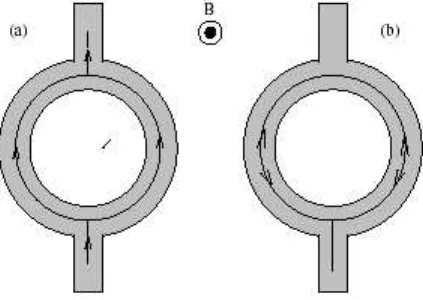
A ring geometry, as the geometry of above calculations, encloses a continuous flux Φ, this results in a fundamental periodicity Φ0 = hc/e. Such a periodicity
is the result of gauge invariance of vector potential. This periodicity comes from interference of trajectories which make one half revolution along the ring, as in figure 1.6.a.
This type currents are sample dependent and have random phases, comes from interference of the trajectories. This type of the Aharonov-Bohm effect can be called the usual Aharonov-Bohm effect, or thermodynamic equilibrium Aharonov-Bohm effect.
I. O. Kulik stated that [6]:
There is no long-range order in this case. The motion of the individual electrons is independent, and the collisions can cause the electrons to become redistributed among the states, but the average current remains different from zero as a consequence of the dependence of the energies of the individual states, and hence of the total energy on ~A.
The current state corresponds in this case to a minimum of the free energy, so that allowance for dissipation does not lead to its decay.
Figure 1.6: Illustration of Aharonov-Bohm effect in a ring geometry. (a) Trajec-tories responsible for hc/e periodicity, (b) trajecTrajec-tories of the pair of time-reversed states leading to hc/2e periodicity.
The second type oscillations originates from time-reversed trajectories. The proper contribution leads to a minimum conductance at ~B = 0. Thus the
oscil-lations have the same phase. They have periodicity hc/2e, so these osciloscil-lations survive in long hollow cylinders. Their origin is a periodic modulation of the weak localization effect due to coherent backscattering. Aharonov-Bohm oscillations in long hollow cylinders were predicted by Altshuler, Aronov, and Spivak [15]. [figure 1.6.b]
In a semiclassical picture these oscillations can be qualitatively understood [16, 17, 18] and have been associated with pairs of time reversed, backscattered paths enclosing the inner disc [22]. This type can be called resistive Aharonov-Bohm effect.
In this thesis first approach is used (also several people who calculated per-sistent currents in carbon nanotubes by using tight binding approximation cal-culated first type of persistent currents).
In a diffusive and thin-walled metallic cylinder (as in long-hollow cylinders), interference of the closed electron trajectories results periodicity of resistance (back-scattering). Phase difference between the trajectory Γ and its time-reversed state Γ0 is ∆Φ = hcΦ/2e = 2Φ/Φ0 = Φ/Φ1, so resistance have oscillation with
period hc/2e (Altshuler, Aronov, and Spivak effect).
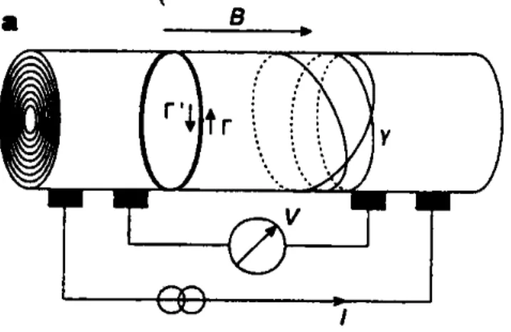
Figure 1.7: Diagram of a MWNT, composed of a series coaxial cylinders. A periodic magneto-resistance is expected to originate from quantum interference of back-scattered electron trajectories
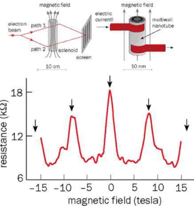
As mentioned before, at zero magnetic field electrical resistance will increase, since interference term add up constructively, effect known as weak localization. Bachtold et. al. measured the electrical transport on multiwalled nanotubes and results illustrated in fig. 1.8. [5]:
Figure 1.8: (Top left) In the standard Aharonov-Bohm effect the magnetic flux through the solenoid changes the relative phase of the electron waves in paths 1 and 2, there is an interference pattern forms on the screen. When the flux is changed, the interference pattern shifts on the screen. (Top right) Carbon nanotube is placed in a magnetic field parallel to the its axis. In the nanotube, there are two paths, clockwise and anticlockwise around the nanotube. These paths interefere and the shift in the interference pattern manifests itself as a change in the electrical resistance along the nanotube as a function of magnetic field (bottom). The magnetic field at the peaks can be related to the quantum of magnetic flux, hc/2e, and the cross-section of the nanotube.
In the compilation of this summary, about Aharonov-Bohm effect, references [19, 20, 8] were also used.
1.3
Kronig-Penney Model
The Kronig-Penney model demonstrates that a simple one-dimensional periodic potential yields energy bands as well as energy band gaps. The periodic potential is shown in the figure 1.7.
The potential is assumed to be periodic in the Kronig-Penney model. The potential barriers with width ζ are spaced by a distance η + ζ. The analysis requires the use of Bloch functions, travelling wave solutions multiplied with a periodic function which has the same periodicity as the potential. Bloch’s
Figure 1.9: periodic potential
theorem helps us to handle the infinite number of interacting electrons moving in a periodic potential, like in the field of an infinite number of ions. Essentially, there are two difficulties to overcome; a wavefunction has to be calculated for each of the infinite number of electrons which will extend over the entire space of the solid, and the basis set, in which the wavefunction is expressed, will be infinite. Periodicity of the potential is the requirement for Bloch’s theorem. Bloch proved that the solutions of the Schr¨odinger equation for a periodic potential must be of the special form [28]
Ψk(r) = uk(r) exp (ik · r)
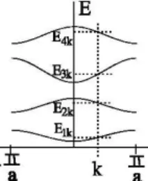
where uk(r) has the period of crystal lattice with uk(r+T) = uk(r). We can express the theorem as, the eigenfunctions of the wave equation for a periodic potential are the product of a plane wave times a periodic function with the periodicity of the crystal lattice. The width η is taken zero, so the potential becomes like in figure 1.7, and energy-band diagram becomes as in figure 1.9 [23, 14].
Figure 1.10: Shaded region indicates allowed energy bands. The band width is indicated by ∆E
Figure 1.11: The ”reduced zone representation” shows that the bands (i.e., the values of k) only range within the First Brillouin Zone (FBZ).The width of the First Brillouin Zone (FBZ) corresponds to the magnitude of the primitive recip-rocal lattice vector.
These calculations will be shown in more detail in the next chapter. As one can compare, same results will be obtained, energy-band diagram will be plotted for different potentials.
1.4
Organization of the Thesis
The thesis is organized as follows: Chapter 2 introduces the helical potential. Two dimensional hamiltonian is solved, energy-band diagram is found for one dimensional Kronig-Penney potential, energy is calculated for full problem, and density of states is calculated. In Chapter 3, Magnetic field is introduced into the Hamiltonian. In addition to the calculations similar to chapter 2, persistent currents are also calculated. In chapter 4, conclusion and future work is presented, finally in chapter 5 compiler ABC is explained.
Part I
2.1
Statement of the Problem
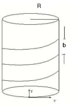
While calculating the persistent currents in nanotubes, many physicists take the problem as electrons move on lattice points along the tube. In this thesis, we assume a helical potential along a cylinder, with the circumference a = 2πR. See figure 2.1. ˆx is the direction along the ring circumference.
Figure 2.1: Potential
The Schr¨odinger Wave Equation for such a problem is:
−¯h2 2µ Ã ∂2Ψ ∂x2 + ∂2Ψ ∂y2 ! + V (x, y)Ψ = εΨ (2.1)
The potential V (x, y) is the helical potential, and as can be seen from the 16
figure this potential is formulated as: V (x, y) = ∞ X n=−∞ δ(y b − x a − n)V0 (2.2)
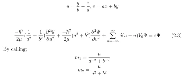
Since potential has both x and y dependence, Hamiltonian is not separable. To make the Hamiltonian separable, variables should be transformed as:
u = y b − x a, v = ax + by −¯h2 2µ ( 1 a2 + 1 b2) ∂2Ψ ∂u2 + −¯h2 2µ (a 2+ b2)∂2Ψ ∂v2 + ∞ X n=−∞ δ(u − n)V0Ψ = εΨ (2.3) By calling; m1 = µ a−2+ b−2 m2 = µ a2+ b2
(note that, m1 and m2 are not the physical masses, they are just parameters
used to simplify calculations)
We get the Hamiltonian as below.
à −¯h2 2m1 ! ∂2Ψ(u, v) ∂u2 + à −¯h2 2m2 ! ∂2Ψ(u, v) ∂v2 + V (u)Ψ(u, v) = εΨ(u, v) (2.4)
Since, H(u, v) = H(u) + H(v), Ψ(u, v) can be written as, Ψ(u, v) = Ψ1(u)Ψ2(v).
If we separate Hamiltonian into two parts we get the following equations.
−¯h2 2m1 µ 1 Ψ1 ¶∂2Ψ 1 ∂u2 + V (u) = ε1 (2.5) and −¯h2 2m2 µ 1 Ψ2 ¶∂2Ψ 2 ∂v2 = ε2 (2.6)
Figure 2.2: V(u), u dependent potential where ε1+ ε2 = ε u dependence: Ã −¯h2 2m1 ! ∂2Ψ 1 ∂u2 + ∞ X n=−∞ δ[u − n]V0Ψ1 = ε1Ψ1 (2.7)
We can use Bloch’s theorem. Since Hamiltonian has periodic potential, V (u+
n) = V (u). In fact this potential is the standard Kronig-Penney potential for
one dimensional case Similar calculations can be found at references [23, 14]. At nth (n − 1 < u < n) region, wavefunction have the form
Ψ1(u) = Anexp[ik1(u − n)] + Bnexp[−ik1(u − n)] (2.8)
whit k1 =
√
2m1ε1/¯h.
At (n + 1)st region: (n < u < n + 1):
Ψ1(u) = An+1exp[ik1(u − n − 1)] + Bn+1exp[−ik1(u − n − 1)]
By using continuity condition at u = n:
An+1exp(−ik1) + Bn+1exp(ik1) = An+ Bn (2.9) An− exp(−ik1)An+1+ Bn− exp(ik1)Bn+1 = 0 (2.10) Integrating equation 2.7: Z n+ε n−ε Ã −¯h2 2m1 Ψ001(u) + ∞ X n=−∞ δ[u − n]V0Ψ1(u) ! du = Z n−ε n−ε ε1Ψ1(u)du
In the limit : ε → 0 Ψ0 1(n + ε) − Ψ01(n − ε) = 2m1 ¯h2 V0Ψ1(n) (2.11) Where the Ψ0
1(n + ε) is the derivative of the solution at the (n + 1)st region
and Ψ0
1(n − ε) is the derivative of the solution at the nth region. If we do the
calculation above, we get the relation:
ik1An+1exp(−ik1)−ik1Bn+1exp(ik1)−ik1An+ik1Bn = 2m1
¯h2 V0(An+Bn) (2.12)
An− exp(−ik1)An+1+ Bn− exp(ik1)Bn+1 = 0 (2.13)
ik1exp(−ik1)An+1− ik1An− 2gAn− ik1exp(ik1)Bn+1+ ik1Bn− 2gBn= 0 (2.14)
where
g = m1V0
¯h2 We can use Bloch condition here:
Ψ1(u + n) = exp(iqn)Ψ1(u)
q is the Bloch wave vector, and it is quantized as:
Ψ1(u + M − 1) = eiq(M −1)Ψ1(u) = Ψ1(u) ⇒ q = 2πl
L
With L = M − 1, since u = y/b − x/a and 0 < y < M · b and 0 < x < a, so 0 < u < M − 1.
Since Ψ(u) is the solution at the nth region, Ψ(u + 1) becomes solution at the
Ψ(u + 1) = An+1exp[ik1((u + 1) − (n + 1))] + Bn+1exp[−ik1((u + 1) − (n + 1))]
= An+1exp[ik1(u − n)] + Bn+1exp[−ik1(u − n)] = exp(iq)Ψ(u)
If we look at the equation 2.8, we see that the above equation is satisfied if:
An+1= exp(iq)An,
Bn+1= exp(iq)Bn.
Figure 2.3: Kronig-Penney relation with positive g value
Figure 2.4: Kronig-Penney relation for negative g, when potential consists wells instead of barriers
So,
(1 − exp(iq − ik1))An+ (1 − exp(iq + ik1))Bn = 0
(ik1exp(iq − ik1) − ik1− 2g) An+ (−ik1exp(iq + ik1) + ik1− 2g) Bn = 0
From these two equations, we get:
cos q = cosk1+
g k1
Figure 2.5: Energy-band diagram for g=0
−1 < cos q < 1, roots for k1 are in between (−1, 1). q is taken between −π and π.
Energy-band diagrams plotted for various g values are shown in figures 2.6-2.11. For computational purposes k1 and q are used, since they are dimensionless
variables, and for the energy below expression is used:
ε1 ε0 = k2 1 Where ε0 = ¯h 2(a2+ b2) 2a2b2µ
Second part of the Hamiltonian has only v dependence:
à −¯h2 2m2 ! ∂2Ψ 2 ∂v2 = ε2Ψ2 (2.16) Ψ2(v) = A exp(ik2v) + B exp(−ik2v) (2.17) where With, k2 = √ 2m2ε2 ¯ h .
Figure 2.6: Energy-band diagram for g=4
Figure 2.7: Energy-band diagram for g=2
Figure 2.9: Energy-band diagram for g=-1
Figure 2.10: Energy-band diagram for g=-2
2.2
Periodic boundary conditions:
Our wavefunction has two periodicities, first is along the axis of cylinder, other along the circumference:
Ψ(x, y + b) = exp(iκ)Ψ(x, y) (2.18)
Ψ(x + a, y) = Ψ(x, y) (2.19)
κ is the longitudinal Bloch wave vector, with the below periodicity:
Ψ(x, y + M · b) = eiκMΨ(x, y) = Ψ(x, y)
κ = 2πm/M, m = 0, 1, ..., M − 1 where L = M · b.
From the relation between the (x, y) and (u, v), periodic boundary conditions can be rewritten for Ψ(u, v):
Ψ(u + 1, v + b2) = Ψ1(u + 1)Ψ2(v + b2) = exp(iκ)Ψ(u, v) (2.20) Ψ(u − 1, v + a2) = Ψ 1(u − 1)Ψ2(v + a2) = Ψ(u, v) (2.21) Since we have: Ψ1(u + n) = exp(iqn)Ψ1(u) We get: Ψ2(v + b2) = exp(iκ − iq)Ψ2(v) (2.22) Ψ2(v + a2) = exp(iq)Ψ2(v) (2.23) Ψ2 = A exp(ik2v) + B exp(−ik2v)
To satisfy boundary conditions, A · B = 0. There are two cases, first B = 0 and second A = 0. For the first case, by using those two boundary conditions, we get the below relation for k2:
k2 =
κ
a2+ b2 (2.24)
For the second case, A = 0, k2 becomes:
k2 =
−κ
a2+ b2 (2.25)
2.3
Summary:
Now we can write the energy ε = ε1+ ε2 as:
εnm = ¯h2k2 1 2m1 +¯h 2k2 2 2m2
(Please note that in this equation k1, k2 are not physical momentums and
m1, m2 not physical masses. They are just used to simplify the calculations.)
εnm = ¯h2(a2+ b2)k2 1 2a2b2µ + ¯h2(a2 + b2)k2 2 2µ Where k1 comes from
cos q = cos k1+ g sin k1/k1
and k2 2 = ( κ a2+ b2) 2
k1, κ and q are dimensionless variables. µ is the physical mass. We can say
physical momentums are:
P = (a 2+ b2 a2b2 ) 1/2k 1(q) Q = (a2+ b2)1/2k 2 = ( κ2 a2+ b2) 1/2
Then energy becomes
εnm =
¯h2P2
2µ + ¯h2Q2
2.4
Density of states:
There are various representations for the density of states, in this case the be-low representation is used, more detailed explanation about this delta function representation can be found at [21].
N(ε) = ∞ X n=1 M −1X m=0 Z π −π dq 2π Z 2π 0 dκ 2πδ(εnm(q, κ) − ε) (2.27) To find the density of states the below property of the delta function is used:
δ(f (x)) =X
i
δ(x − xi)
|f0
(xi)|
xi’s are the zeros of the function f (x).
By applying this rule, it can be shown that:
N(ε) = ∞ X n=1 M −1X m=0 X i Z Ldσ 1 |ˆudεnm dq + ˆv εnm dκ |εnm(q,κ)i=ε (2.28)
where L is the line of εnm− ~k plot and σ is the surface of this plot. ~k is the
the wave vector.
~k = ˆuq + ˆvκ
Accurate analytical result for the density of states is not calculated, instead it is calculated numerically.
While calculating the density of states numerically the program ABC is used. Same program is also used to calculate the energy. MATLAB is used for plotting. For density of states we calculated the number of states at an energy interval.
In the following pages, for different values of g number of states is plotted, both for negative and positive values of g:
Figure 2.13: Density of States for g=6
Figure 2.14: Density of States for g=4
Figure 2.16: Density of States for g=-2
Figure 2.17: Density of States for g=-4
Part II
In this part, magnetic field is introduced into the Hamiltonian. First we assume a magnetic field parallel to the ˆy direction. The field is confined into a solenoid.
The vector potential is assumed to have magnitude only in ˆx direction. Later we
assume that the cylinder is curved as to make a toroid and there is a magnetic field parallel to the toroid axis. This magnetic field is also confined in a solenoid. The vector potential can be assumed to have magnitude only in ˆy direction. Below
figure is taken to compare the coordinates that are used in the calculations, with the cylindrical coordinates. ˆx direction that is used in my calculations corresponds
to r ˆθ direction, ˆy direction corresponds to ˆz direction and ˆz direction corresponds
to ˆr direction.
Figure 3.1: Cylindrical coordinates
3.1
Magnetic Field Parallel to the Cylinder
Axis, ~
B
αMagnetic field, ~Bα, is parallel to the ˆy direction. From the Stokes theorem:
Z S ~ Bα· d~a = Z S(∇ × ~A) · d~a = I ~ A · d~s = Φ
So Aα = Φaα. The transformation for px is made, px → px− eAcα.
−¯h2 2µ Ã ( ∂ ∂x − ie ¯hcAα) 2+ ∂2 ∂y2 ! Ψ + V (x, y)Ψ = EΨ (3.1) Figure 3.2: ~Bα
By making necessary transformations u = y b − x a and v = ax + by: −¯h2 2µ Ã a2+ b2 a2b2 ∂2 ∂u2 + 2ieAα ¯hca ∂ ∂u + (a 2+ b2) ∂2 ∂v2 − 2ieAαa ¯hc ∂ ∂v − e2A2 α ¯h2c2 ! ψ+V (u)ψ = Eψ (3.2) Now the Hamiltonian is separable, it divides into two parts
à −¯h2 2m1 ( ∂ ∂u + ieAαab2 ¯hc(a2+ b2)) 2+ V 0 ∞ X n=∞ δ(u − n) ! Ψ1(u) = ε1Ψ1(u) (3.3)
−¯h2 2m2 ( ∂ ∂v − ieAαa ¯hc(a2+ b2)) 2Ψ 2(v) = ε2Ψ2(v) (3.4)
where m1 and m2 have the same values as before, and ε1+ ε2 = ε.
First equation has the Kronig-Penney potential term, as solved before. Ψ1(u)
has the solution at nth region:
Ψ1(u) = Anei(k1− eAαab2 ¯ hc(a2+b2))(u−n)+ B ne−i(k1+ eAαab2 ¯ hc(a2+b2))(u−n) (3.5) k1 = √ 2m1ε1 ¯h
This eigenfunction also satisfies Bloch condition, since potential is periodic. Ψ1(u + n) = exp(iqn)Ψ1(u)
and
An+1= exp(iq)An,
Bn+1= exp(iq)Bn.
By using the continuity condition at u = n:
An+1ei(k1−∆1)(−1)+ Bn+1e−i(k1+∆1)(−1) = An+ Bn
applying Bloch condition:
(e−i(k1−∆1−q)− 1)A n+ (ei(k1+∆1+q)− 1)Bn= 0 (3.6) where ∆1 = eAαab 2 ¯ hc(a2+b2). Z n+ε n−ε Ã −¯h2 2m1 ( ∂ ∂v + ieAαa ¯hc(a2+ b2)) 2+ X∞ n=−∞ δ[u − n]V0Ψ1(u) ! du = Z n−ε n−ε ε1Ψ1(u)du In the limit : ε → 0 Ψ0 1(n + ε) − Ψ01(n − ε) = 2m1 ¯h2 V0Ψ1(n)
As in previous calculations, in Part I, Ψ0
1(n+ε) is the derivative of the solution
at the (n + 1)st region and Ψ0
1(n − ε) is the derivative of the solution at the nth
region. After the calculations the below result is obtained:
(i(k1 − ∆1)e−i(k1−∆1−q)− i(k1− ∆1) − 2g)An+ (−i(k1+ ∆1)ei(k1+∆1+q)
+i(k1+ ∆1) − 2g)Bn(3.7)
after combining above equations and calling g = m1V0
¯
h2 one can easily obtain:
cos (q + ∆1) = cos k1+ g sin k1 k1 (3.8) Figure 3.3: g = 1, (cos γ)2 Φα Φ0 = 1 2 Figure 3.4: g = 1, (cos γ)2 Φα Φ0 = 1 3 v dependence: Ψ2(v) = Aei(k2+∆2)+ Be−i(k2−∆2) (3.9) ∆2 = eAαa ¯hc(a2+ b2), k2 = √ 2m2ε2 ¯h
3.1.1
Periodic boundary conditions:
Periodicity conditions are the same as in Part I:
Ψ(x, y + b) = exp(iκ)Ψ(x, y) (3.10)
Ψ(x + a, y) = Ψ(x, y) (3.11)
Ψ2(v + b2) = exp(iκ − iq)Ψ2(v) (3.12)
Ψ2(v + a2) = exp(iq)Ψ2(v) (3.13)
To satisfy the boundary conditions, A · B = 0. For B = 0:
k2 = κ a2+ b2 − ∆2 (3.14) second case, A = 0: k2 = −κ a2+ b2 + ∆2 (3.15) Since we need k2
2 to calculate ε2 the result will be the same for both cases.
3.1.2
Summary:
εnm = ε1+ ε2 = ¯h2k2 1 2m1 +¯h 2k2 2 2m2 E = nF X n=1 MF X m=0 Z q00 q0 dq 2π( ¯h2(a2+ b2) 2µa2b2 k 2 1+ ¯h2 2µ(a2+ b2)(κ − eΦα ¯hc ) 2) (3.16)With the relation:
cos(q + eΦαb
2
¯hc(a2+ b2)) = cos k1+ g
sin k1
q0 and q00 are determined by the number of electrons, they are simply equal to −π and π up to fermi level.
We can call cos γ = √ b
a2+b2. Flux quantum Φ0 =
hc
e, will be inserted into the
equations.
Figure 3.5: b = L/M and a is the circumference of the cylinder Where κ is longitudinal Bloch wave vector, as mentioned before.
κ = 2πm/M, m = 0, 1, ..., M − 1 L = Mb (so 0 < κ < 2π) E = nF X n=1 MF X m=0 Z q00 q0 dq 2π( ¯h2(a2 + b2) 2µa2b2 k 2 1 + ¯h2 2µ( 2πm M − 2πΦα Φ0 )2) cos(q + (2π cos γ) 2Φ α Φ0 ) = cos k1+ g sin k1 k1
Periodicity of the ε1n and ε2m can be shown directly:
ε1n(Φα+
Φ0
(cos γ)2) = ε1n(Φα)
ε2m(Φα+ Φ0) = ε2(m−M )(Φα)
(Please note that in this equation k1, k2 are not physical momentums and
m1, m2 not physical masses. They are just to use to simplify the calculations.)
P = (a2+ b2 a2b2 ) 1/2k 1(q), Q = (a2+ b2)1/2k2 Energy becomes εnm = ¯h2P2 2µ + ¯h2Q2 2µ (3.17)
3.1.3
Density of states:
Density of states calculations are also similar to Part I.
N(ε) = ∞ X n=1 M −1X m=0 Z π −π dq 2π Z 2π 0 dκ 2πδ(εnm(q, κ) − ε) (3.18) N(ε) = ∞ X n=1 M −1X m=0 X i Z Ldσ 1 |ˆudεnm dq + ˆvεdκnm|εnm(q,κ)i=ε (3.19) where L is the line of εnm− ~k plot. ~k is the the wave vector.
~k = ˆuq + ˆvκ
Figure 3.6: g=1, Φα = 4Φ0, with b = 1, a =
√
3.1.4
Persistent Currents:
Persistent currents calculated here are due to thermodynamic equilibrium, mini-mum of free energy occurs when there is non-decaying current. Below calculations are similar to those shown in the introduction part.
Inm= −c∂εnm
∂Φα
First contribution to the current (I1):
∂ε1 ∂Φα = ∂ε1 ∂k1 ∂k1 ∂Φα ∂ ∂Φα (q + eΦαb 2 ¯hc(a2+ b2)) = ∂k1 ∂Φα ∂ ∂k1 (arccos(cos k1+ g sin k1 k1 )) ∂ε1 ∂Φα = −¯h 2eb2k 1 ¯hc(a2+ b2)m 1 · q 1 − (cos k1+ g sin k1/k1)2
sin k1− g cos k1/k1+ g sin k1/k12
= (3.20) −¯he a2cµ · k2 1 q k2 1 − (k1cos k1+ g sin k1)2 k2
1sin k1 + gk1cos k1+ g sin k1
(3.21)
Second contribution to the current (I2):
∂ε2 ∂Φα = ∂ ∂Φα ( ¯h 2 2µ(a2+ b2)(κ − eΦα ¯hc ) 2) ∂ε2 ∂Φα = ¯he µc(a2+ b2)(κ − eΦα ¯hc ) (3.22) Inm= ¯he cµ · ( 1 a2 k2 1 q k2 1 − (k1cos k1+ g sin k1)2 k2
1sin k1+ gk1cos k1+ g sin k1
− 1
a2+ b2(κ −
eΦα
Total current can be written as: I = nF X n=1 MF X m=0 Z q00 q0 dq 2π ¯he cµ · ( 1 a2 k2 1 q k2 1 − (k1cos k1+ g sin k1)2 k2
1sin k1 + gk1cos k1+ g sin k1
− 1
a2+ b2(κ −
eΦα
¯hc )) (3.24) By looking at above equations one can easily say
I1n(Φα+
Φ0
(cos γ)2) = I1n(Φα)
I2m(Φα+ Φ0) = I2(m−M )(Φα)
3.2
Additional Magnetic Field, Perpendicular
to the Cylinder Axis, ~
B
βWhen magnetic field is parallel to the axis of the torus obtained by curving the cylinder:
Figure 3.8: ~Bβ is the along the direction perpendicular to the torus axis, ~Aβ is
along the cylinder, ˆy axis.
~
Bβ = ∇ × ~Aβ = Aβ∇ × ˆy
From the Stokes theorem:
Aβ = Φβ M · b py → py − eAβ c −¯h2 2m à ( ∂ ∂x − ie ¯hcAα) 2) + ( ∂ ∂y − ie ¯hcAβ) 2) ! Ψ + V (x, y)Ψ = EΨ (3.25)
à −¯h2 2m1 ( ∂ ∂u − iea2b2 ¯hc(a2+ b2)( Aβ b − Aα a )) 2+−¯h2 2m2 ( ∂ ∂v − ie ¯hc(a2+ b2)(aAα+ bAβ)) 2 ! Ψ(u, v) +V(u)Ψ(u, v) = εΨ(3.26) à −¯h2 2m1 ( ∂ ∂u + i∆1) 2+ V 0 ∞ X n=∞ δ(u − n) ! Ψ1(u) = ε1Ψ1(u) (3.27) −¯h2 2m2 ( ∂ ∂v − i∆2) 2Ψ 2(v) = ε2Ψ2(v) (3.28)
So we have the same equations as in the ~Bα case, except constants ∆1 and
∆2. ∆1 = ea2b2 ¯hc(a2+ b2)( Aα a − Aβ b ) = e ¯hc(a2 + b2)(b 2Φ α− a2 MΦβ) ∆2 = e ¯hc(a2+ b2)(aAα+ bAβ) = e ¯hc(a2 + b2)(Φα+ 1 MΦβ) Figure 3.9: g = 1, (cos γ)2 Φα Φ0 = (cos γ) 2 Φβ Φ0 = 1 3, M = 10
Ψ1(u) = Anei(k1−∆1)(u−n)+ Bne−i(k1+∆1)(u−n) (3.29)
cos (q + ∆1) = cos k1 + g
sin k1
k1
(3.30)
3.2.1
Periodic boundary conditions:
Periodicity and wavefunctions are same, except, the value of constant ∆2.
To satisfy the boundary conditions, A · B = 0. For B = 0:
k2 = κ a2+ b2 − ∆2 (3.32) second case, A = 0: k2 = −κ a2+ b2 + ∆2 (3.33)
3.2.2
Summary:
εnm = ε1+ ε2 = ¯h2k2 1 2m1 +¯h 2k2 2 2m2 E = nF X n=1 MF X m=0 Z q00 q0 dq 2π( ¯h2(a2+ b2) 2µa2b2 k 2 1) + ( ¯h2e µ¯hc(a2+ b2)(κ − Φα− 1 MΦβ) 2) cos(q + e ¯hc(a2+ b2)(b 2Φ α− a2 MΦβ)) = cos k1+ g sin k1 k1We can recall cos γ = √ b
a2+b2. Flux quantum Φ0 =
hc
e, will be inserted into
the equations.
Where κ is longitudinal Bloch wave vector, κ = 2πm/M, m = 0, 1, ..., M − 1. (L = Mb, so 0 < κ < 2π) E = nF X n=1 MF X m=0 Z π −π dq 2π( ¯h2(a2+ b2) 2µa2b2 k 2 1 + ¯h2 2µ( 2πm M − ( 2πΦα Φ0 +2πΦβ MΦ0 ))2) cos(q + 2π((cos γ) 2Φ α Φ0 ) + (sin γ) 2Φ β MΦ0 )) = cos k1+ g sin k1 k1
Periodicity of the ε1n and ε2m can be shown directly: ε1n(Φα+ Φ0 (cos γ)2) = ε1n(Φα) ε1n(Φβ+ MΦ0 (sin γ)2) = ε1n(Φβ) ε2m(Φα+ 2mΦ0 M ) = ε2(m−M )(Φα) ε2m(Φβ + 2mΦ0) = ε2(m−1)(Φβ)
(Please note that in this equation k1, k2 are not physical momentums and
m1, m2 not physical masses. They are just to use to simplify the calculations.)
εnm = ¯h2(a2+ b2)k2 1 2a2b2µ + ¯h2(a2 + b2)k2 2 2µ Physical momentums are:
P = (a 2+ b2 a2b2 ) 1/2k 1(q) Q = (a2+ b2)1/2k 2 Energy becomes εnm = ¯h2P2 2µ + ¯h2Q2 2µ (3.34)
3.2.3
Density of states:
Density of states calculations are also similar to Part I.
N(ε) = ∞ X n=1 M −1X m=0 Z π −π dq 2π Z 2π 0 dκ 2πδ(εnm(q, κ) − ε) (3.35)
Figure 3.10: g=1, Φα = Φβ = 2Φ0, with b = 1, a = √ 2, M = 10. N(ε) = ∞ X n=1 M −1X m=0 X i Z Ldσ 1 |ˆudεnm dq + ˆvεdκnm|εnm(q,κ)i=ε (3.36) where L is the line of εnm− ~k plot. ~k is the the wave vector.
3.2.4
Persistent Currents:
Calculations are similar to chapter 2. But this time there are two persistent currents caused by two vector potentials, ~Aα, ~Aβ:
Inm(Φα) = −c ∂εnm ∂Φα Inm(Φβ) = −c ∂εnm ∂Φβ
Inm(Φα) has the same value as before:
I(Φα) = nF X n=1 MF X m=0 Z q00 q0 dq 2π ¯he cµ·( 1 a2 k2 1 q k2 1 − (k1cos k1+ g sin k1)2 k2
1sin k1+ gk1cos k1+ g sin k1
− 1
a2 + b2(κ−
eΦα
¯hc )) (3.37)
Inm(Φβ) nearly same as the previous value, except constants:
I(Φβ) = nF X n=1 MF X m=0 Z q00 q0 dq 2π (−¯he) Mcµ ·( 1 a2 k2 1 q k2 1 − (k1cos k1+ g sin k1)2 k2
1sin k1+ gk1cos k1 + g sin k1
− 1 M(a2 + b2)(κ− eΦα ¯hc )) (3.38) I1n(Φα+ Φ0 (cos γ)2) = I1n(Φα) I1n(Φβ+ MΦ0 (sin γ)2) = I1n(Φβ) I2m(Φα+ 2mΦ0 M ) = I2(m−M )(Φα) I2m(Φβ + 2mΦ0) = I2(m−1)(Φβ)
Figure 3.11: Persistent current I1, found for Φα = Φβ, electrons fill 3/4 of the
Conclusions and Future Work
In this thesis we tried to calculate the persistent currents in carbon nanotubes exactly, instead of using tight-binding approximation. First carbon nanotubes are studied to learn the structure deeply. Then Aharonov-Bohm effect is stud-ied to learn the persistent currents and its types. The Kronig-Penney model, which helps us to solve the periodic structures such as atoms in a crystal, is also reviewed.
Trying to solve the problem exactly brought some difficulties, as I know no similar method was used before. In the literature all the calculations were made by using tight-binding approximation.
First the helical potential is introduced and the Schr¨odinger equation is solved when there is no magnetic field. We choose the potential V (x, y), since it is helical and exactly solvable, even it does not exactly fit with the real system. Although the problem seems to be a simple one, it has physical importance.
Later, we numerically calculated the energy-band gap and density of states. The program ABC is used. As a second step magnetic field is introduced into the problem. We performed similar calculations as in part one and additionally we calculated the persistent currents. The calculated current has two terms, first term is periodic in Φ, but second does not seem to be periodic. By looking at
similar representations for persistent currents, it seems that, after calculating thermally averaged current, this problem will be eliminated.
Later, we investigated the persistent currents in a torus which is made by curving the cylindrical conductor. An additional magnetic field is applied, and we recalculated energy, density of states, and persistent currents for this case. This time there were two contribution to the current, one from Φα and the other
from Φβ.
With this project, persistent currents and carbon nanotubes attracted my interest. In the future I am planning to finish all the calculations related to this thesis (i.e. thermally averaged current) and compare my results with the calculations made by using tight binding approximation [24, 29]. I will also search the applications [26, 27].
Appendix
5.1
ABC
In this thesis the compiler ABC is used. ABC, Advanced Basic/C Com-piler/Convertor/Programmer produces C-codes and executables. It works in var-ious hardware/software environments (Windows, Linux and UNIX machines). The ABC C-code is translated from the QuickBasic environment source code. It is suitable for various mathematical routines such as complex numbers, ar-bitrary precision arithmetics, multidimensional integration, eigenvalue problem for sparse and conventional complex Hermitian matrices, etc (The dimension of matrix can be up to 1.000.000 if executed on a standard Pentium PC). ABC assumes a mathematical subspace of Basic environment as it was specified in the Microsoft QuickBasic. By using the QuickBasic compiler as an editor,there is an additional advantage of testing the initial program code for possible errors by trying to execute (but not actually executing) the program thus eliminating most of (possible) syntax errors. The ABC code accepts complex numbers, special functions, arbitrary precision floating-point variables and a number of standard (and some times new) mathematical algorithms written in compliance with the (pseudo) QuickBasic dielect, so that the error checking is also applicable to these QuickBasic extensions within the QuickBasic rules. As an example, below is a
program in ABC:
DIM a; b; c; x; y AS DOUBLE : a = 0.111 : b = 0.222 c = integ(x,0,1,y,1-x,1+x,(Sin(pi*a*x*y+b))2
print a;b;c
So problem calculates the integral:
c = Z 1 0 dx Z 1+x 1−x dy(sin(πaxy + b)) 2
In case when program execution is assumed on a machine different from the one of the ABC, the C-code appropriate to that machine is generated. The codes thus produced are generally equal, or faster, than the conventional C-codes on same machine. Unlike similar programs for mathematical calculations (Maple or Matlab), ABC doesn’t support any sophisticated graphics. Also, dynamic strings are limited to the scope necessary for easy communication with the com-piler. The goal is rather in easy programming for non-professionals (physicists, mathematicians), on a professional level. Special algorithms are implemented in the routine library of ABC. In particular the eigenvalue problem for extremely large sparse Hermitian matrices, and user friendly routines for multi-dimensional numeric integration etc. [25].
As an example below routine is our density of states calculation: DIM rr, g, k, q, qmin, qmax, kap, kapmin, kapmax, eps AS DOUBLE DIM i, m, n, nn, mm, ii AS LONG DIM delE, ldoub, emax AS DOUBLE, DIM l, num AS LONG
eps = 10−10
INPUT ”nn,mm,ii,g,num =”; nn, mm, ii, g, num
DIM etot(nn, mm, ii) AS SINGLE
qmin = -pi: qmax = pi kapmin = 0: kapmax = 2 * pi
FOR m = 1 TO mm: q = qmin + (qmax - qmin) * (m - 1) / (mm - 1) FOR n = 1 TO nn
r(n, m) = root(k, (n - 1) * pi, n * pi, COS(k) + g * SIN(k + eps) /(k + eps) - COS(q)) E(n, m) = (r(n, m))2
FOR i = 1 TO ii kap = kapmin + (kapmax - kapmin) * (i - 1) / (ii - 1) NEXT i: NEXT n: NEXT m
emax = 0
FOR m = 1 TO mm: FOR n = 1 TO nn: FOR i = 1 TO ii q = qmin + (qmax - qmin) * (m - 1) / (mm - 1) rr = r(n, m) kap = kapmin + (kapmax - kapmin) * (i - 1) / (ii - 1)
etot(n, m, i) = rr 2+ kap2
IF etot(n, m, i) > emax THEN emax = etot(n, m, i) NEXT i: NEXT n: NEXT m
emax = 1.1 * emax delE = emax / num
DIM D(num) AS SINGLE, X(num) AS SINGLE FOR n = 1 TO num D(n) = 0: NEXT n
FOR n = 1 TO num: X(n) = emax * n / num: NEXT n FOR m = 1 TO mm: FOR n = 1 TO nn: FOR i = 1 TO ii
ldoub = etot(n, m, i) / delE l = INT(ldoub)
IF l > 0 THEN D(l) = D(l) + 1 NEXT i NEXT n: NEXT m num = plot(D, X)
OPEN ”dos2.m” FOR OUTPUT AS 1 PRINT 1, ”X=[” FOR n = 1 TO num PRINT 1, X(n): NEXT n PRINT 1, ”];” PRINT 1, ”D=[”
FOR n = 1 TO num: PRINT 1, D(n): NEXT n PRINT 1, ”];”
PRINT 1, ”plot(X,D,’-’);” PRINT 1, ”xlabel(’E’);” PRINT 1, ”ylabel(’N(E)’);”
PRINT 1, ”title(’Density of states’);” CLOSE 1
OPEN ”energy1.m” FOR OUTPUT AS 1 PRINT 1, ”q=[” FOR m = 1 TO mm
q = qmin + (qmax - qmin) * (m - 1) / (mm - 1) PRINT 1, q(m) NEXT m
PRINT 1, ”];” PRINT 1, ”E=[”
FOR m = 1 TO mm FOR n = 1 TO nn
r(n, m) = root(k, (n - 1) * pi, n * pi, COS(k) + g * SIN(k + eps) / (k + eps) - COS(q)) E(n, m) = (r(n, m))2
PRINT 1, E(n, m): NEXT n: NEXT m PRINT 1, ”];”
PRINT 1, ”plot(q,E,’-’);” PRINT 1, ”xlabel(’q’);” PRINT 1, ”ylabel(’E’);”
PRINT 1, ”title(’Energy-band diagram’);” CLOSE 1
[1] S. Ijima, Helical microtubules of graphitic carbon, Nature, 354, 56, (1991). [2] C. Schonenberger, L. Forro, Multiwall Carbon Nanotubes, Physics World,
June, (2000).
[3] C. Dekker, Carbon Nanotubes as molecular quantum wires Physics Today, May, 22-28, (1999).
[4] M. Dressselhaus et al., Carbon Nanotubes, Physics World, January, (1998). [5] A. Bachtold et al., Aharonov-Bohm oscillations in carbon nanotubes, Nature,
397, 673-678, (1999).
[6] I. O. Kulik, Pis’ma Zh. Eksp. Teor. Fiz., 11, 407, (1970). [JETP Letters, 11, 275, 1970.]
[7] M. B¨uttiker, Y. Imry, R. Landauer, Physics Letters, 96A, 365, (1983). [8] I. O. Kulik, Magnetic and Electric Aharonov-Bohm Effects in Nanostructers,
Physica B, 218, 252, (1996).
[9] I. O. Kulik, ”Transverse” persistent currents in mesoscopic cylinders and
rings, Physica B, 284, 1880-1881, (1996).
[10] I. O. Kulik, R. Ellialtioglu, Mesoscopic Phenomena and Mesoscopic Devices
in Microeletronics, Kluwer Academic Publishers, Netherlands, (2000).
[11] V. Chandrasekhar et. al., Phys. Review Letters, 67, 3578, (1991).
[12] L. P. L´evy, G. Dolan, J. Dunsmuir, H. Bouchiat, Phys. Review Letters, 64, 2074, (1990).
[13] Y. Aharanov, D. Bohm, Physical Review, 115, 485, (1959).
[14] C. Kittel, Introduction to Solid State Physics,Wiley, New York, (1986). [15] B. L. Altshuler, A. G. Aronov, B. Z. Spivak, Pi’sma Zh. Eksp. Teor. Fiz.,
23, 101, (1981). [JETP Lett. 33, 94, 1981.]
[16] H.U. Baranger, R.A. Jalabert, A.D. Stone, Chaos, 3, 665, (1993).
[17] K. Richter, Semiclassical Theory of Mesoscopic Quantum Systems, Springer, Berlin, (2000).
[18] R.A. Jalabert, New Directions in Quantum Chaos, IOS Press, Amsterdam, (2000).
[19] B. Washburb, R. A. Webb, Aharonov-Bohm effect in normal metal:
Quan-tum Cohenrence and Transport, Adv. Phys., 35, 375, (1986).
[20] Y. Imry, Introduction to Mesoscopic Physics, Oxford University Press, Ox-ford, (1997).
[21] W. Ashcroft, N. D. Mermin, D. Mermin, Solid State Physics, International Thomson Publishing, (1976).
[22] S. Kawabata, K. Nakamura, Phys. Review, B57, 6282, (1998).
[23] Stephen Gasiorowicz, Quantum Physics, John Wiley and Sons, Singapore, (1974).
[24] M.F. Lin, D. S. Chuu, Persistent Currents in Torodial Carbon Nanotubes, Phys. Review B, March, (1998).
[25] I. O. Kulik, Hopping and Correlation Effects in Atomic Clusters and
Net-works, ICCN Publications, (2001).
[26] A. Barone, T. Hakioglu, I. O. Kulik, preprint con-mat/0203038. [27] I. O. Kulik, T. Hakioglu, A. Barone, Eur. Phys. J., B30, (2002).
[28] J. J. Sakurai, Modern Quantum Mechanics, Addison-Wesley Publishing Comp., (1998).
[29] H.F. Cheung, E.K. Riedel, Y. Gefen, Persistent currents in mesoscopic rings