Optimization of orders in multichannel fractional
Fourier-domain filtering circuits and its application
to the synthesis of mutual-intensity distributions
I˙mam S¸amil Yetik, Mehmet Alper Kutay, and Haldun Memduh Ozaktas
Owing to the nonlinear nature of the problem, the transform orders in fractional Fourier-domain filtering configurations have usually not been optimized but chosen uniformly. We discuss the optimization of these orders for multi-channel-filtering configurations by first finding the optimal filter coefficients for a larger number of uniformly chosen orders, and then maintaining the most important ones. The method is illustrated with the problem of synthesizing desired mutual-intensity distributions. The method we propose allows those fractional Fourier domains, which add little benefit to the filtering process but increase the overall cost, to be pruned, so that comparable performance can be attained with less cost, or higher performance can be obtained with the same cost. The method we propose is more likely to be useful when confronted with low-cost rather than high-performance applications, because larger im-provements are obtained when the use of a smaller number of filters is desired. © 2002 Optical Society of America
OCIS codes: 070.6560, 070.2590.
1. Introduction
The fractional Fourier transform has found many applications in optics and signal processing.1–19 A
comprehensive exposition to the subject and an ex-tensive bibliography may be found in Ref. 20. The
ath order fractional Fourier-transform operation
cor-responds to the ath power of the ordinary Fourier-transform operation. If we denote the ordinary Fourier-transform operator byᏲ, then the ath-order fractional Fourier-transform operator is denoted by Ᏺa. Standard eigenvalue methods for finding a
function G共Ꮽ兲 of a linear operator Ꮽ can be employed to obtain an explicit formula for the transform. If the eigenvalue equation of Ꮽ is Ꮽn共u兲 ⫽ nn共u兲,
we define G共Ꮽ兲 through the eigenvalue equation
G共Ꮽ兲n共u兲 ⫽ G共n兲n共u兲. The eigenvalue equation of
the Fourier transform isᏲn共u兲 ⫽ exp共⫺in兾2兲n共u兲,
wheren共u兲, n ⫽ 0, 1, 2, . . . are the set of Hermite– Gaussian functions: 21兾4共2nn!兲⫺1兾2Hn共公2u兲
exp共⫺u2兲, where H
n共u兲 are the standard Hermite
polynomials. Now, using the above approach, the fractional Fourier transform can be defined in terms of the eigenvalue equation Ᏺan共u兲 ⫽ 关exp共⫺in兾
2兲兴a
n共u兲. We choose to resolve the ambiguity in the
ath power function as关exp共⫺in兾2兲兴a ⫽ exp共⫺ian兾
2兲. To find the fractional Fourier transform of an arbitrary square-integrable function f共u兲 we first ex-pand it in terms of the complete orthonormal set of functionsn共u兲 and then apply the above eigenvalue
equation to each term of the expansion. After rear-ranging the terms and using a standard identity for Hermite polynomials关Ref. 20, table 2.8.9兴, it is pos-sible to show that the ath-order fractional Fourier transform fa共u兲 ⬅ Ᏺa f共u兲 of the original function is
given by fa共u兲 ⫽
冋
1⫺ i cot冉
a 2冊册
1兾2兰
exp再
i冋
cot冉
a 2冊
u 2 ⫺ 2 csc冉
a 2冊
uu⬘ ⫹ cot冉
a 2冊
u⬘ 2册冎
f共u⬘兲du⬘. (1) The zeroth-order fractional Fourier transform of a function is the function itself and the first-orderI˙. S¸ . Yetik, is with the University of Illinois at Chicago, Depart-ment of Electrical and Computer Engineering, Chicago, Illinois. M. A. Kutay is with TU¨ BITAK-UEKAE共Scientific and Technical Research Council of Turkey–National Research Institute of Elec-tronics and Cryptology兲 TR-06100 Kavaklidere, Ankara, Turkey. H. M. Ozaktas is with Bilkent University, Department of Electrical Engineering, TR-06533 Bilkent, Ankara, Turkey.
Received 6 March 2001; revised manuscript received 11 January 2002.
0003-6935兾02兾204078-07$15.00兾0 © 2002 Optical Society of America
transform is equal to the ordinary Fourier transform. Positive and negative integer values of a simply cor-respond to the repeated application of the ordinary forward and inverse Fourier transforms respectively. The fractional Fourier-transform operator satisfies the index additivity:Ᏺa2Ᏺa1⫽ Ᏺa2⫹a1. The operator
Ᏺais periodic in a with period 4 becauseᏲ2equals the
parity operator, which maps f共u兲 to f共⫺u兲 and Ᏺ4
equals the identity operator.
An important concept in Fourier analysis is the Fourier共or frequency兲 domain. This domain is un-derstood to be a space where the Fourier-transform representation of f共u兲 lives. The space-frequency plane 共also known as phase space兲 is the plane spanned by the space共u兲 and spatial frequency 共兲 coordinates 关Fig. 1共d兲兴. The horizontal axis is the space domain where f共u兲 lives. The vertical axis is the frequency or Fourier domain where the Fourier transform F共兲 lives. In general, oblique axes ua
making angle␣ ⫽ a兾2 with the u axis are the order fractional Fourier domains, where the ath-order fractional Fourier transforms fa共ua兲 live. This
notion is supported by the fact that fractional Fourier transformation corresponds to rotation of certain space-frequency distributions, such as the Wigner distribution, and that the integral projection of the Wigner distribution on the ua axis yields the ath-order fractional Fourier energy density.20 –25
The ath-order discrete fractional Fourier trans-form faof a given N⫻ 1 vector f is found as fa⫽ F
a
f,
where Fa is the N ⫻ N discrete fractional Fourier-transform matrix,26 which is essentially the ath
power of the ordinary discrete Fourier-transform ma-trix F. If the discrete vectors represent the samples of their continuous counterparts and if N is chosen equal to or greater than the space-bandwidth product of f共u兲, the discrete fractional transform approxi-mates the continuous fractional transform in the same way as the ordinary discrete transform approx-imates the ordinary continuous transform.
2. Fractional Fourier-Domain Filtering
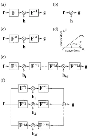
Space- and frequency-domain filtering are special cases of fractional Fourier-domain filtering 共Figs. 1共a兲, 1共b兲, 1共c兲兴.24,27 Fractional Fourier-domain
fil-tering consists of 共i兲 taking the fractional Fourier transform of the input signal,共ii兲 multiplication with a filter function, and共iii兲 taking the inverse fractional Fourier transform of the result. The fractional ver-sion of the optimal Wiener filtering problem has been studied in detail.27,28 Fractional Fourier-domain
fil-tering has been further generalized to multistage and multichannel filtering关Figs. 1共e兲 and 1共f 兲兴. In mul-tistage filtering29 –33 the input is first transformed
into the a1th domain, where it is multiplied by a filter
h1. The result is then transformed back into the
original domain. This process is repeated M times. Denoting the diagonal matrix corresponding to mul-tiplication by the kth filter hkby Ak, we can write the
following expression for the overall effect of the mul-tistage filtering configuration:
Tms⫽ F⫺aM⌳M· · · Fa2⫺ a1⌳1Fa1, (2)
where Tms is a matrix representing the overall
multi-stage-filtering configuration and Fak is the
akth-order discrete fractional Fourier-transform
matrix. Multi-channel-filtering configurations31–35
consist of M single-stage blocks in parallel. For each channel k, the input is transformed to the akth
do-main, multiplied by a filter hkand then transformed
back. We can write the following expression for the overall effect of the multi-channel-filtering configuration: Tmc⫽
兺
k⫽1 M F⫺ak⌳ kFak, (3)where Tmcis a matrix representing the overall multi-channel-filtering configuration. It is possible to fur-ther generalize these filtering configurations by use of parallel and series arrangements together; such systems have been called generalized filtering cir-cuits.36
Fractional Fourier transform-based filtering cir-cuits have found applications in many areas in-cluding optical and digital signal and image
Fig. 1. 共a兲 Fourier-domain filtering. 共b兲 Space-domain filtering. 共c兲 ath-order fractional Fourier domain filtering. 共d兲 Fractional Fourier domains. 共e兲 Multistage filtering. 共f 兲 Multichannel fil-tering.
restoration, signal and system synthesis, synthesis of mutual-intensity distributions, and fast implementa-tion of shift-variant linear systems 共Ref. 20, Chap. 10兲.
The problem of finding the optimal filter coeffi-cients, given the transform orders, was solved.27,30,33
Given a matrix H that represents a system one wishes to synthesize, one seeks the filter coefficients such that the resulting matrices Tms or Tmcare as
close as possible to H according to some specified criteria, such as mean square error. Until now the transform orders have usually been chosen uni-formly; the problem of optimizing the orders has not yet been addressed. In this paper we show how one can optimize over the orders for multichannel filtering by first finding the optimal filter coeffi-cients for a larger number of uniformly chosen or-ders and then maintaining the most important ones.
Fractional Fourier-transform-based filtering con-figurations have been used for approximating linear space-variant systems, represented by some matrix
H.30 –32,34 It was shown that for many such
sys-tems encountered in various applications, it is possible to approximate the system H with a mul-tistage or multichannel configuration Tms or Tmc
with acceptable mean square error, by using a small or moderate number M of stages or channels. Be-cause the cost of implementing the fractional Fou-rier transform 共optically or digitally兲 is similar to the cost of implementing the ordinary Fourier transform, this leads to an efficient implementation of the space-variant system in question. For
digi-tal systems, the cost is of the order of MN log N, which should be compared to a cost of the order of
N2 for direct implementation of linear systems.
共Here N is the length of the discrete signal vectors that should be at least as large as the space-bandwidth product of the continuous signals.兲
In the multichannel case it is possible to analyti-cally find the optimal filter coefficients, provided that the transform orders are given.33 In practice,
how-ever, an iterative method is preferred. In the mul-tistage case it is not possible to find analytic solutions, so an iterative method must be used to begin with.30
In this paper we concentrate on the multi-channel-filtering case and consider the improvement of opti-mizing over the M orders in addition to the filter coefficients. We first find the optimal filter coeffi-cients for a larger number P of uniformly chosen orders and then maintain the most important ones. More specifically, we start with P uniformly chosen orders, where P is several times the number of orders
M we are eventually going to use. Then the M or-ders resulting in filters with the highest energies are chosen, and the other P–M branches of the mul-tichannel configuration are eliminated. Finally, with the M orders thus chosen, we reoptimize the filter coefficients.
Figure 2 shows how the fractional Fourier-transform stages of the multichannel configuration can be optically implemented.21,37–39 Either of the
alternative implementations shown 关in Figs. 2共b兲, 2共c兲, or 2共d兲兴 can be used for the fractional Fourier blocks appearing in Fig. 2共a兲. For a fractional
trans-Fig. 2. 共a兲 The multichannel configuration consists of k ⫽ 1, 2, . . . , M parallel channels, each consisting of a fractional Fourier-transform stage Fakfollowed by a spatial filter h
kfollowed by another fractional Fourier-transform stage of order⫺ak. 共b兲, 共c兲 and 共d兲 show three
alternative optical implementations of the fractional Fourier-transform stages appearing in共a兲 共b兲 Canonical implementation type I. 共c兲 Canonical implementation type II. 共d兲 Quadratic graded-index 共GRIN兲 medium implementation. While the focal lengths of the lenses and their separations are shown in共b兲 and 共c兲 the radial-refractive-index distribution is given by n2共r兲 ⫽ n
0
form of order a, the parameters of the configurations should be chosen as follows:
Fig. 2共b兲: dI⫽ s2 tan共a兾4兲, fI⫽ s2 csc
冉
a 2冊
, (4) Fig. 2共c兲: dII⫽ s2 sin共a兾2兲, fII⫽ s2 cot冉
a 4冊
, (5) Fig. 2共d兲: dGRIN⫽ s2 共a兾2兲, GRIN ⫽ s2 , (6) where is the wavelength and s is a suitably chosen scale parameter with the dimension of length. These configurations will map a function f共x兾s兲 at their input to a function fa共x兾s兲 at their output, wherex is measured in meters.
3. Synthesis of Mutual-Intensity Distributions
To illustrate our approach, we will consider the prob-lem of synthesizing light with a desired mutual in-tensity. Here we wish to synthesize a system H such that, when light of a given mutual intensity is present at the input, light whose mutual intensity is as close as possible to the given specification is ob-tained at the output. Choosing to work with one-dimensional signals taking dimensionless variables for simplicity, we let f共u兲 and g共u兲 denote the input and output optical fields, and Rf共u1, u2兲 and Rg共u1, u2兲 denote the input and output mutual intensities. If
f共u兲 and g共u兲 are the input and output of a system
characterized by a kernel H共u, u⬘兲 such that g共u兲 ⫽ f
H共u, u⬘兲f共u⬘兲 du⬘, then the input and output mutual
intensities are related by
Rg共u1, u2兲 ⫽
兰兰
Rf共u1⬘, u2⬘兲 H共u1, u1⬘兲⫻ H*共u2, u2⬘兲du1⬘du2⬘ , (7)
where H* denotes the complex conjugate of H. The sampled, discrete version of the optical fields will be represented by column vectors f and g and the mu-tual intensity functions will be represented by matri-ces Rfand Rg. Then, we have g⫽ Hf, where H is the
discrete form of the system kernel and the double integral relationship above assumes the following matrix form:
Rg⫽ HRfH†, (8)
where H†is the Hermitian conjugate of H. Equation
共8兲 is quadratic in H. We are going to employ an equivalent representation that is linear. Because mutual intensity matrices R are Hermitian and pos-itive semi-definite, it is possible to diagonalize them as
R⫽ UDU†, (9)
where D is a diagonal matrix whose elements are the real eigenvalues, and U is a matrix whose columns constitute the set of orthonormal eigenvectors of R so that U†U ⫽ I, where I is the identity matrix.
Let-ting D1兾2denote the diagonal matrix whose elements are the positive square roots of the elements of D, we substitute D1兾2U†UD1兾2for D in the above equation:
R⫽ UD1兾2U†UD1兾2U†. (10)
Using this expansion for both Rgand Rf, we can write
Rg⫽ R˜gR˜g†⫽ R˜gR˜g⫽ R˜g2, (11) Rf⫽ R˜fR˜f†⫽ R˜fR˜f⫽ R˜f2, where R˜g⫽ R˜g †⫽ UD1兾2U† , (12) R˜f⫽ R˜f †⫽ UD1兾2U† .
Substituting Eq.共11兲 into Eq. 共8兲 we obtain the fol-lowing: R˜gR˜g † ⫽ HR˜fR˜f † H†. (13)
One way of satisfying the above equation is to en-sure that
R˜g⫽ HR˜f, (14)
or
H⫽ R˜gR˜f⫺1. (15)
In our numerical examples, we are going to con-sider the input light source to be incoherent. As-suming this source extends uniformly from⫺r0to r0,
its mutual intensity can be written as
Rf共u1, u2兲 ⫽ ␦共u1⫺ u2兲rect
冉
u1
2r0
冊
. (16) When discretized, the corresponding matrix Rf共and its square root R˜f兲 is equal to the identity I provided
that r0 is larger than the interval over which we sample. Therefore the matrix H we wish to approx-imate is simply equal to R˜g.
As a first example, we wish to synthesize a Gaussian–Schell-model beam with mutual intensity:
Rg共u1, u2兲 ⫽ exp
冋
⫺ 共u1⫺ u2兲2 2r12册
exp冉
⫺u1 2⫹ u 22 4r22冊
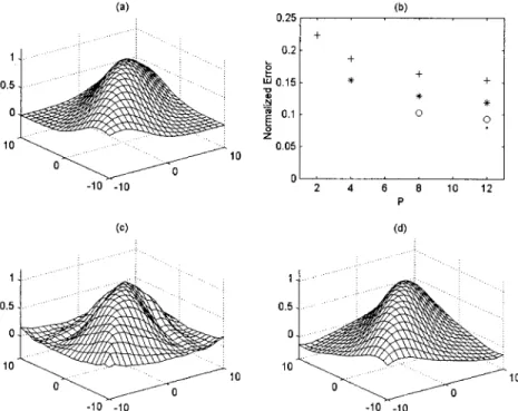
. (17) 共In our examples r1 ⫽ 5 and r2 ⫽ 10.兲 When wesynthesize the filter H corresponding to this mutual intensity using the multichannel configuration with
M⫽ 3 filters 共a1⫽ 1兾3, a2 ⫽ 2兾3, a3 ⫽ 1兲, the
nor-malized error turns out to be 15.42 %. Using the proposed method of optimizing the orders with P⫽ 12, we find that the optimal orders are a1 ⫽ 2兾12,
a2 ⫽ 5兾12, a3 ⫽ 10兾12, and the normalized error
using these orders becomes 12.64 %. When we syn-thesize the same H with M⫽ 2 filters 共a1⫽ 1兾2, a2⫽
orders with P⫽ 8, we find that the optimal orders are
a1 ⫽ 2兾8, a2 ⫽ 6兾8, and the normalized error using
these orders is 16.36%. Further simulations have been undertaken for other values of M and P and the resulting errors are plotted in Fig. 3共b兲. Figure 3共a兲 shows the desired mutual intensity, Fig. 3共c兲 shows the synthesized mutual intensity for M⫽ 2 without optimization of orders, and Fig. 3共d兲 shows the syn-thesized mutual intensity for M⫽ 2 with optimiza-tion of orders with P⫽ 8.
As a second example we consider the synthesis, as closely as possible, of a mutual-intensity profile spec-ified as Rg共u1, u2兲 ⫽ rect
冉
兩u1⫺ u2兩 2r1冊
rect冉
u1 2r2冊
rect冉
u2 2r2冊
, (18) where r2 ⬎ r1. This amounts to specifying theam-plitude of light at two points to be fully correlated when the distance between those points is less than
r1, and totally uncorrelated otherwise. Because the rectangle function does not represent a physically realizable mutual-intensity function共it is not positive semi-definite兲, its negative eigenvalues will be re-placed by zero in obtaining its square root represen-tation. This amounts to replacing the rectangle function with the closest positive semi-definite func-tion. When we synthesize the filter H corresponding to this mutual intensity using the multichannel con-figuration with M ⫽ 3 filters 共a1 ⫽ 1兾3, a2 ⫽ 2兾3,
a3⫽ 1兲, the normalized error is 15.35 %. Using the
proposed method of optimizing the orders with P⫽ 12, we find that the optimal orders are a1 ⫽ 2兾12,
a2 ⫽ 6兾12, a3 ⫽ 10兾12, and the normalized error
using these orders is 12.3 %. When we synthesize the same H with M⫽ 2 filters 共a1⫽ 1兾2, a2⫽ 1兲, the
normalized error is 22.64 %. Optimizing the or-ders with P⫽ 8, we find that the optimal orders are
a1 ⫽ 2兾8, a2 ⫽ 6兾8, and the normalized error using
these orders is 15.45 %. Once again, further simu-lations were undertaken for other values of M and P and are plotted in Fig. 4共b兲. Figure 4共a兲 shows the desired mutual intensity, Fig. 4共c兲 shows the synhthesized mutual intensity for M ⫽ 2 without optimization of orders, and Fig. 4共d兲 shows the syn-thesized mutual intensity for M⫽ 2 and optimization of orders with P⫽ 8.
A number of conclusions can be drawn by examin-ing the numerical results. First, optimization of the orders is capable of offering tangible improvements compared to choosing the orders uniformly. We also observe that beyond a certain value of P, further increases in this parameter do not offer further re-ductions in the error共the benefits of optimizing over the orders is saturated兲. This is because further in-creasing P merely allows further refinements and fine tuning in choosing the optimal orders that which have a diminishing return once one is already close to the optimal orders. Also, we can see that improve-ments coming from optimization of the orders are greater when M is smaller but less when M is larger. This is because when M is large to begin with, it is already possible to concentrate the filtering action in those domains that are optimal. This of course means that the other domains add cost to the system implementation with little benefit, and the method
Fig. 3. 共a兲 Desired Gaussian–Schell-model mutual intensity profile. 共b兲 Normalized error versus P for different values of M. We show
M⫽ 2, P ⫽ 2, 4, 8, 12 by crosses; M ⫽ 4, P ⫽ 4, 8, 12 by asterisks M ⫽ 8, P ⫽ 8, 12 by open circles, and M ⫽ 12, P ⫽ 12 by dots. 共c兲
we propose is useful precisely because it allows these low benefit domains to be pruned.
4. Conclusion
In conclusion, we have presented a simple and effec-tive way of optimizing the orders in fractional Fourier-domain-based multi-channel-filtering config-urations. Until now, the orders had mostly been chosen uniformly because there was no simple way of solving the nonlinear problem of optimizing over the orders. The method we propose is more likely to be useful when confronted with low-cost, rather than high-accuracy applications, because larger improve-ments are obtained when the use of a smaller number of filters is desired. Future work might include ex-tending the method to the multistage case, which poses a number of challenges, and to more general filtering circuits. Generalizing the procedure to the optimization of the parameters of linear canonical transform-based-filtering systems,40 which are even
more general than fractional Fourier-transform-based systems, would have the potential to offer fur-ther improvements.
References
1. L. B. Almeida, “The fractional Fourier transform and time-frequency representations,” IEEE Trans Signal Process. 42,
3084 –3091共1994兲.
2. O. Akay and G. F. Boudreaux-Bartels, “Unitary and Hermitian fractional operators and their relation to the fractional Fourier transform,” IEEE Signal Process. Lett. 5, 312–314共1998兲. 3. T. Alieva, V. Lopez, F. Agullo-Lopez, and L. B. Almeida, “The
fractional Fourier transform in optical propagation problems,” J. Mod. Opt. 41, 1037–1044共1994兲.
4. I˙. S¸ . Yetik, H. M. Ozaktas, B. Barshan, and L. Onural, “Per-spective projections in the space-frequency plane and frac-tional Fourier transforms,” J. Opt. Soc. Am. A 17, 2382–2390 共2000兲.
5. L. M. Bernardo and O. D. D. Soares, “Fractional Fourier trans-forms and imaging,” J. Opt. Soc. Am. A 11, 2622–2626共1994兲. 6. W. X. Cong, N. X. Chen, and B. Y. Gu, “Recursive algorithm for phase retrieval in the fractional Fourier transform domain,” Appl. Opt. 37, 6906 – 6910共1998兲.
7. D. Dragoman and M. Dragoman, “Near and far field optical beam characterization using the fractional Fourier tansform,” Opt. Commun. 141, 5–9共1997兲.
8. M. F. Erden, H. M. Ozaktas, and D. Mendlovic, “Propagation of mutual intensity expressed in terms of the fractional Fourier transform,” J. Opt. Soc. Am. A 13, 1068 –1071共1996兲. 9. M. F. Erden, H. M. Ozaktas, and D. Mendlovic, “Synthesis of
mutual intensity distributions using the fractional Fourier transform,” Optics Commun. 125, 288 –301共1996兲.
10. J. Garcı´a, R. G. Dorsch, A. W. Lohmann, C. Ferreira, and Z. Zalevsky, “Flexible optical implementation of fractional Fou-rier transform processors. Applications to correlation and fil-tering,” Opt. Commun. 133, 393– 400共1997兲.
11. S. Granieri, R. Arizaga, and E. E. Sicre, “Optical correlation based on the fractional Fourier transform,” Appl. Opt. 36, 6636 – 6645共1997兲.
12. J. Hua, L. Liu, and G. Li, “Scaled fractional Fourier transform and its optical implementation,” Appl. Opt. 36, 8490 – 8492 共1997兲.
13. C. J. Kuo and Y. Luo, “Generalized joint fractional Fourier transform correlators: a compact approach,” Appl. Opt. 37, 8270 – 8276共1998兲.
14. S. Liu, J. Xu, Y. Zhang, L. Chen, and C. Li, “General optical implementation of fractional Fourier transforms,” Opt. Lett.
20, 1053–1055共1995兲.
15. A. W. Lohmann, Z. Zalevsky, and D. Mendlovic, “Synthesis of Fig. 4. 共a兲 Closest positive semi-definite approximation to the desired rectangular mutual intensity profile. 共b兲 Normalized error versus
P for different values of M. We show M⫽ 2, P ⫽ 2, 4, 8, 12 by pluses; M ⫽ 4, P ⫽ 4, 8, 12 by asterisks M ⫽ 8, P ⫽ 8, 12 by open circles, and M⫽ 12, P ⫽ 12 by dots. 共c兲 Synthesized profile using uniform orders 共M ⫽ 2兲. 共d兲 Synthesized profile using optimized orders 共M ⫽ 2, P⫽ 8兲.
pattern recognition filters for fractional Fourier processing,” Opt. Commun., 128, 199 –204共1996兲.
16. D. Mendlovic, Z. Zalevsky, and H. M. Ozaktas, “Applications of the fractional Fourier transform to optical pattern recogni-tion,” in Optical Pattern Recognition,共Cambridge University Press, Cambridge, 1998兲 Chap. 4, pp. 89–125.
17. P. Pellat-Finet, “Fresnel diffraction and the fractional-order Fourier transform,” Opt. Lett. 19, 1388 –1390共1994兲. 18. Z. Zalevsky, D. Medlovic, and H. M. Ozaktas, “Energetic
effi-cient synthesis of general mutual intensity distribution,” J. Opt. Soc. A 2, 83– 87共2000兲.
19. Y. Zhang and B.-Y. Gu, “Rotation-invariant and controllable space-variant optical correlation,” Appl. Opt. 37, 6256 – 6261 共1998兲.
20. H. M. Ozaktas, Z. Zalevsky, and M. A. Kutay, The Fractional
Fourier Transform with Applications in Optics and Signal Processing,共John Wiley & Sons, New York, 2001兲.
21. A. W. Lohmann, “Image rotation, Wigner rotation, and the fractional order Fourier transform,” J. Opt. Soc. Am. A 10, 2181–2186共1993兲.
22. A. W. Lohmann and B. H. Soffer, “Relationships between the Radon–Wigner and fractional Fourier transforms,” J. Opt. Soc. Am. A 11, 1798 –1801共1994兲.
23. D. Mustard, “The fractional Fourier transform and the Wigner distribution,” J Aust. Math. Soc. B 38, 209 –219共1996兲. 24. H. M. Ozaktas, B. Barshan, D. Mendlovic, and L. Onural,
“Convolution, filtering, and multiplexing in fractional Fourier domains and their relation to chirp and wavelet transforms,” J. Opt. Soc. Am. A 11, 547–559共1994兲.
25. H. M. Ozaktas, B. Barshan, and D. Mendlovic, “Convolution and filtering in fractional Fourier domains,” Opt. Rev. 1, 15–16 共1994兲.
26. C¸ . Candan, M. A. Kutay, and H. M. Ozaktas, “The discrete fractional Fourier transform,” IEEE Trans. Signal Process. 48, 1329 –1337共2000兲.
27. M. A. Kutay, H. M. Ozaktas, O. Arikan, and L. Onural, “Op-timal filtering in fractional Fourier domains,” IEEE Trans. Signal Process. 45, 1129 –1143共1997兲.
28. Z. Zalevsky and D. Mendlovic, “Fractional Wiener filter,” Appl. Opt. 35, 3930 –3936共1996兲.
29. M. F. Erden, M. A. Kutay, and H. M. Ozaktas, “Repeated filtering in consecutive fractional Fourier domains and its ap-plication to signal restoration,” IEEE Trans. Signal Process.
47, 1458 –1462共1999兲.
30. M. F. Erden and H. M. Ozaktas, “Synthesis of general linear systems with repeated filtering in consecutive fractional Fou-rier domains,” J. Opt. Soc. Am. A 15, 1647–1657共1998兲. 31. M. A. Kutay, M. F. Erden, H. M. Ozaktas, O. Arikan, O¨ .
Gu¨ leryu¨ z, and C¸ . Candan, “Space-bandwidth-efficient realiza-tions of linear systems,” Opt. Lett. 23, 1069 –1071共1998兲. 32. M. A. Kutay, M. F. Erden, H. M. Ozaktas, O. Arikan, C¸ .
Can-dan, and O¨ . Gu¨leryu¨z, “Cost-efficient approximation of linear systems with repeated and multi-channel filtering configura-tions,” in Proceedings of the 1998 IEEE International
Confer-ence on Acoustics, Speech, and Signal Process. 共IEEE,
Piscataway, N. J., 1998兲 pp. 3433–3436.
33. M. A. Kutay, H. O¨ zaktas¸, M. F. Erden, H. M. Ozaktas, and O. Arikan, “Solution and cost analysis of general multi-channel and multi-stage filtering circuits,” in Proceedings of the 1998
IEEE-SP International Symposium on Time-Frequency and Time-Scale Analysis共IEEE, Piscataway, N. J., 1998兲 pp. 481–
484.
34. M. A. Kutay, H. O¨ zaktas¸, H. M. Ozaktas, and O. Arikan, “The fractional Fourier domain decomposition,” Signal Process. 77, 105–109共1999兲.
35. I˙. S¸ . Yetik, M. A. Kutay, H. O¨ zaktas¸, and H. M. Ozaktas, “Continuous and discrete fractional Fourier domain decompo-sition, “in Proceedings of the 2000 IEEE International
Confer-ence on Acoustics, Speech, and Signal Processing, 共IEEE,
Piscataway, N. J., 2000兲 Vol. I, pp. 93–96.
36. H. M. Ozaktas, M. A. Kutay, and D. Mendlovic, “Introduction to the fractional Fourier transform and its applications” in P. W. Hawkes, ed., Advances in Imaging and Electron Physics, Vol. 106共Academic Press, San Diego, Calif., 1999兲 Chap. 4, pp. 239 –291.
37. D. Mendlovic and H. M. Ozaktas, “Fractional Fourier trans-forms and their optical implementation: I, J. Opt. Soc. Am. A
10, 1875–1881共1993兲.
38. H. M. Ozaktas and D. Mendlovic “Fractional Fourier trans-forms and their optical implementation: II.” J. Opt. Soc. Am. A
10, 2522–2531共1993兲.
39. H. M. Ozaktas and D. Mendlovic, “Fractional Fourier optics,” J. Opt. Soc. Am. A 12, 743–751共1995兲.
40. B. Barshan, M. A. Kutay, and H. M. Ozaktas, “Optimal filter-ing with linear canonical transformations,” Opt. Commun.