Optimal control of a two-stage stochastic hybrid manufacturing system with Poisson arrivals and exponential service times

Proceedings of the

44th IEEE Conference on Decision andControl,and theEuropeanControl Conference 2005

Seville, Spain,December12-15,2005

ThlAI

9.6

Optimal

Control

of

a

Two-Stage Stochastic

Hybrid

Manufacturing System

with

Poisson

Arrivals

and

Exponential

Service Times

Kagan Gokbayrak and Omer Selvi

Abstract- Extending earlier work on single-stage stochastic hybrid system models, we consider atwo-stagestochastichybrid systemwhere thejob arrivalsarerepresented throughaPoisson process,and theservice times required to attainadesiredphysical

state areexponentially distributed dependentonthe controllable process rates. For the case where the costs associated with the process ratesand theinventory levels arenon-decreasing convex, and the process rates take values from finite sets, we show that thereexist thresholdpoliciesonbothinventory levels forselecting theoptimal process rates ateach station.

Index Terms-Stochastic, Hybrid Systems, Two-Stage, Opti-mal Rate Control

I. INTRODUCTION

The term "hybrid" is used to characterize systems that include time-driven and event-driven dynamics. The former

are represented by differential (difference) equations, while the latter may be describedthrough various frameworks used for Discrete Event Systems (DES), such as timed automata, max-plus equations, queueing networks, or Petri nets(see[1]). Broadly speaking, two categories of modeling frameworks have beenproposedtostudy hybridsystems: Those that extend event-driven models to include time-driven dynamics; and those that extend the traditional time-driven modelsto include event-driven dynamics (for an overview, see [2], [3], [4], [5])

The hybrid system modeling framework used in this paper falls into the first category above and is motivated by the

structure of many manufacturing systems. In these systems, discrete entities (referred to asjobs) move through anetwork of work-centers which process thejobs so as to change their

physical characteristics according to certain specifications.

Associated with eachjob are aphysical state and atemporal

state. The physical state

zij

evolves accordingto time-driven

dynamics modeled through differential equations Zi,j =

fj(Zi,j,ui,j)

for i

Zij(Tinj) = j Zij(Ti,j + Si,j)

1,2,...

,md

,

(1)

(2) which, depending on the particular problem being studied,

describe changes in such quantities as the temperature, size, weight, chemical composition, bacteria level, or some other

measure of the "quality" of thejob. The temporal state ofa

K. Gokbayrak and 0. Selvi are with the Department of Indus-trial Engineering, Bilkent University, Ankara, Turkey kgokbayr, selvi@bilkent.edu.tr,

job evolves according to event-driven dynamics, e.g., by the Lindley Equation (see in [1])

xijl =

mnax(ai,

ix-1,2)+ si,i Xi,2 =

max(xi,l,,xi-1,2)

+Si,2

xo, =-0 (3) X0,2=- O (4) and includes information such as the arrival time

ai,

departure

times

xij,

and service times

sij

of job i at work-center j dependent on the control input uij applied on job i to

bring it to a desired final state

(icj.

The interaction of time-driven with event-time-driven dynamics leads to a natural trade-off between temporal requirements on job completion times and physical requirements on the quality of the completed jobs. For example, while the physical state of ajob can be madearbitrarily close to a desired"qualitytarget," thisusually

comes at the expense of long processing times resulting in

excessive inventory costs or violation of constraints on job completiondeadlines. Ourobjective,therefore, istoformulate and solveoptimalcontrolproblemsassociated with such trade-offs.

In [6], [7], [8], and [9], the hybrid system framework is adopted to analyze a single-stage manufacturing process

assuming a deterministic setting, i.e., a known job arrival schedule and controllable service times for alljobs. An ef-ficient algorithm to determine the optimal service times for

a class of single-stage systems is presented in [8]. In [10], however, a stochastic model of a single-stage manufacturing

system is studied, where the job arrivals are represented through a Poisson process with the control variable being

the exponential service's process rate. Adopting an M/M/1

queueing model to describe the event driven dynamics, it is shown that when theinventory-level-dependentservice process

ratestake values fromafinite set, and thecostsassociated with the process rate and the inventory level are non-decreasing

convex, there exists athresholdpolicy on the inventorylevel forselectingthe optimalprocessrate. Inthis paper,weextend the model in [10] to a two-stage hybrid system model and show that similar threshold policies exist on inventory levels for each station.

II. PROBLEM FORMULATION

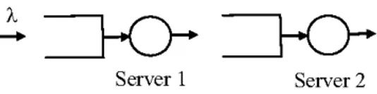
Consider thetwostageserialmanufacturing systemdepicted

in Figure 1. Jobs are arriving to the system according to a

Server 1 Server 2 Fig. 1. Two-stageserial manufacturing system

at a time on a first-come first-served non-preemptive basis (i.e. a job in service can not be interrupted until its service

completion). Service times for both servers are exponentially

distributed and server 1 (1 = 1,2) operates with rate u1 E U1

where

Ul

's arefinite sets such that

U1 =

(5)12

m

The rates uv are indexed so that uv <u + for i 1,...,m

1-1.

Defining a rate = A+

ul1

H+ u 2, this system can be modeled as a discrete-time Markov Chain(DTMC). The state

space for this DTMC canbe defined as

S {(i,j):i,j2o+}

where the state

(i,j)

describes the system with i jobs in the first server and j jobs in the second server. The transition probabilities for this DTMC are

P(oAo)

(ki ) 1- A ly

P(i,o),(k,l)

{

P(o,j),(k,l)

{ 1 1

P(i,j),(kil)

A u (i,O) A±u1 (i,O) 0 +u2(O j) A±U2(O,i) 0 A u1 (ii) u2(2ij) j

I _ A+uI(i,j)+U2 (i,j)

0

(k,l )

=

(1,0)

(k,l )

=

(0, 0)

otherwise

(k,l )

=

(i

+

1,

O)

(k,l )

=

(i-

1:

l)

(k,l )

=

(i: 0)

otherwise

(k,l)

=

(I,j)

(k,l )

=

(O,

j-

1)

(k,l )

=

(O,j

) otherwise

(k,l)=(i

+ l,j)

(k,l)

=(i

-l,j +

1)

(k,l )

=

(i

j-1)

(k,l )

=

(i,j

) otherwise

Assuming that the servers start with system sizes q , the infinite horizon problem we consider is to determine the

stationary state-dependent rate setting policy w such that the discounted cost

is minimized. Note that in(6), a is the discount factor,

ql

denotes the system size for server1, and the pair

(UIl

z2)

=

7(ql,

q2)

denotes thecorrespondingpolicy-determinedprocess ratesfor the servers. The one step cost

C(ql,q2,uI,

2)

in (6) is assumed to be separable, i.e.,

C(ql,Q2,

'Uk

2)

=

bi(ql)

+

b2(q2)

+C,(k

+U2(u)

where the inventory costs

bl

(.) and the service costs cj (.) are

non-decreasing convex functions.

III. OPTIMAL RATE CONTROL POLICY

Applying DynamicProgramming (DP),ine.g. [1I1],tosolve theoptimal controlproblem (6), the discounted cost-to-go DP

equation for state (i,j ) becomes

Vn+l(i,j)

=

Imin

1(iij) U1 I 2(i,j) U2

bi(i)

+b2(j) +ci(u1(i,j)) + c2(U2(i,j)) +a Vn(i - 1,j)

+e

(

jVn

(i-1j

+

1)

U-aV

(i,j)

A±1 (i'i) u(ij)vV

A+u (i,j)+U (i,j E i

(7)

Notethat for all i,j,n E

+,

we have assumed

Vn(-i,j

+

1)

=

Vn(0J)

and Vnt(u -1i) = Vnn( ) Let us define A

Vn")

(i,j)

AV142)

(i,j)

Vn(ij

)

Vn(ij

)

Vn(i-Vn(izj

(8) (9)

i,j

+

1)

- 1)

By (8) and (9), for all i,j,n Ei

Z+

AV

)(0,j)

=

AV12)(i,0)

=0

The following theorem establishes theoptimal control pol-icy:

Theorem 1. The optimalcontrols for the

(n

+

l)th

step are

ul

+1(i,j)

= arg min cl

(u1)

n

~~

0UI1U

Un+

1(i,j)

arg

mnm

fC2(U2)

aUAVi{2)(i,j2}

u2EU2

Proof:

The cost-to-go equation in (7) can be writtenas

Vn+l(i,j)

bj(i)

+

b2(j)

+H

aVn(i,j)

A

H-a

[Vn(iH-1J) -Vn(i,j)

+_u1(i,j)Emin U + min U2(i,j) U2 (6)

ci(u1(i,j))

-au

(yijAV,,)(')

)

c2(U2(i,j

))

_

()\Vn(2)(ij

-)X -au2 A t I'

uI

ce 'Av(1)

(i

j

)

IT n Do 2) =E,

2,U

1 2)

Vx

(q

1.q x

a'C(ql,q

u 0 0

E

k k O k ,k=O -i

Hence, the result follows. U

Corollary 1. The optimal rates for empty servers are the lowest cost rates for those servers, i.e.,

u1(0j

)

arg m {CdUh} 1

U1 UI U1

u2(i,

0)

arg

min

{c2()}

=

Proof. Since AVn1 (O,j) and AVn2 (i,

O)

are zero for all i,j E

E+,

the result follows from Theorem 1. U Since it is

computationally

impossible to solve for

ni\1)

(i,j) and A'V( (i,j) over all i ,j and n, determining

the optimal process rates for all states (i,j)

analytically

is not feasible. Instead, we will exploit monotonicity

properties

of

AV4(1)(i,j)

and I\(

2)(i,j)

to establish

inventory

level thresholds for the optimalprocess rates.

Using notation

cl

=

cl(ul

),

we can define the thresholds

,1

as C ±1 Clk W=t-k+l k k

k=1

a('.

{DO

k= 0 0<k<mn k=ml

Given thatcl

(.)

isanon-decreasingconvex

function,

31

is also

non-decreasing in k for 1= 1, 2, which allows us to establish

the following optimality condition:

Lemma 1. The optimal process rate

ul(i,j)

ul

if and

only if/31 A<

V$ti,j)

</3A Proof: (<=) Let us assume that

i3- <

AV(0

)(i,j

)<

ol

and Then,

ct

-

a-"

(iUA

jV )

<c1 Ift>k then k <AV)(i,j) Ift<k then

which contradicts the u (i,j)

AVn')(i,j

) <i3

k-1

u5 assumption. Similarly, if )Ck Ck-1 a Kl_tk -CUl-1

_-k-I

then c1 -a

kIV(

(ij)

<c1

which contradicts the u1

(i,j

) u5 assumption. U An immediate corollary ofLemma 1 is the following: If

AVn()(ii,j1)

<

AVn(l)4(i2,j2)

then the optimal process rates

satisfy

ul

(i',

j1) <

Ul (i2,j 2).

Depending on the

[k35 k35]

interval that the

AVVn4

(i,j)

values fallin, an optimal process rate

ul

is selected.

The following theorem establishes monotonicity properties

of the

A17jjt)(i,j)

and implies the existence of a threshold

policy.

Theorem 2. Given

b(.)

and

c(.)

as non-decreasing convex

functions, for all i,j,n E Z+

i)

AIV1

(i,(j)

isnon-decreasing ini and

non-increasing

in

,X,

i.e.,

A V(1)(ij) A

V(1)

(it

3

AV1)(i+

1,j)

>

AVn)

(i.j

-+

1) ii)

AVn42)

(i,j)

is non-decreasing inboth i andj,

i.e.,

AV2)(i,j)

AV\2)

(i,j

)

Proof: (By Induction)

Let us define

K -vV(i+,j)

AVn

(i2,j+I )

'6V1 j (1)

A=/ijV(

(i

-+

l,j)

-AiV(')

'6Vk,i,j

()=

AV(')(i,j

+31)

AV()

We needto show that for all k

Vkl,i,j(1)

>

0,6V

kij(2)

<0

5Vk

k,(1)

> 0,61

i,j(2)

>0 For k =0, since

Vo(i,j)

=0 for all

i,j,

(i,j) (i,)

I >

A\V(0)(inj)

Ct

Vol,

i

(1)

6V2Oij

j(1)

0V_0:0

O1i,j

₀

_ij

_j(2)

(2)

Both casescontradict our assumption, so the optimalprocess

rate u (i,j ) = u .

(=>)Conversely, let us assume that ul(i,j) = ul and consider the following cases: If

KCk±1 CkA

1 i- J

Uk

±1

Uk

Next, assume that for k = n, for all i,j

n,i,j

(2)

< O n,i,j

(2)

> O

We needto show that for k =n+1 and for all i,j

then 0,V

n+l±i,j

(2) <0

6,V

2+

i(2)

> O

\

V(0)

(

i:

j)

>0

II

Cl

-a-'\kVn(l)(i,j)

>C1 _{a +}

IAVn(4)

_(ij)

iVnn+a

iaI

( )

>s

6Vn+l

)i,

j()

>

inequalities

are satisfied.

U~1 k I a_ckcl 0 0 Uk -..) a 'A

Vn(l)

(t

3 IT

!.k

-. ) a 'A

Vn(l)

(t

3 IT

c1

ol<

t k 1 aut

6Vn',i,j

(1)

>-6

Vn,

i,i

(1)

>-M,V

M,V

j+2

j+l-

I-i-i

(ub,C ) _~~~~

(ud

cd)

(ug

cg)

~~r- ~--~ ~-IC

ifC

,

(Uf

Cf

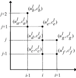
uj--i-i i i+l

Fig.2. Optimalprocessratesand theircosts forstep (n+1)

Let us assume that optimal process rates from Theorem 1 and their costs are calculated

(given

in

Figure

2.)

Then,

AV(')<(i,j)

and

AV(21(i,j)

can be given as

A1

+aeAV({)

(i,j) +ae iVj(1)

U1

cHa

+ e aAV1

4l(i

1,j

+

1)

2

+C2H-_a

adAV1(2)(i1j

H

-Ca

2H+

-aV()(i- l,Va +1)

AV(2)

( j)=b(j) 2(j1) +

CeAV(2)

(in bC

H-cceaLddAV42)(i,i

+-a

b2AV(

ij i)

+Ce-w>

n\n(nd

L2

=[V(i2j

Hi)

-V(i2j

)1

-[Vn(iH- l,j) -Vn(i Hij+i)1

2

- j(2) >

hence byLemma 1 u 2(iH 1,j) <u

2+(i,j

+

1)

holds for all i,j. This enables us toclaim the

following

inequalities:

uI <

ul

<

ul

<

ul

<

ul

< u XU1b - <ia1 1 K Ld1 K-Li1UK Lif1

,I < <u<<u2<

Step 1: (Proof of

5V±1+lij

(1) > 0)

We have

6VIn+l,i,j

()=

[b,I(

+1)-b

Ii][b, ()b

I

i1)]

+Ha A

6ni+,,j

(1) + T

H1

+ T where

ULm = H aa (5V ,j±

I(1)

ml a~~1

T(1)

=0e

unH

u)

igj

(1) + AV ij()I 1

I.

6Vn,

i j (I

[(Ct

cl)

-aLi

LAV()(ij

d H-i)]

(l)~ un,u V

~ ~

1)

+ °

Ua'AV(lI)(ij-l()(

2 U2

Li1

2 aim2 Li91 6 u2 2 Ha a 9

1Vj21(1)

H-

[(c2

c2)

-aLi

di/AV(2)(ij)1

(c~ c) -a

Note that we can

manipulate (12)

to derive an

equivalent

definition for

t(1)

t 2 2 aLi2 a(5V 2 IT

~a-Vn,i+lj

(1) >ITan

2-

2 . Vce9 1(2) I n,i+ l,j-1(2 ) a 2 C2 U2)V2 +(CaCd ITa2 2

[

2~c)

_(Li2

Li)AV(2)

(i,j

H)

Observe that

1. Since

bi (.)

is

non-decreasing

convex in

i',

2.

By

the induction

hypothesis,

a-6

+l,j(1)

> 0

3.

By

the induction

hypothesis,

and since

uL~

>

uLi

Lie

_a

Li961

Lie16

4. a. If u

=ud,

then (cI cd) a Li Hence,

Ld

\(l)(

j)

₀ 4. b. If

ul

>u then IT

(CI

n - d -a(ul -d) -ud~

1)

Hence, (cg- c) -a g AV (ij) > 0 5. a. If

ul

= Ul, then a~

~1

(C

-CD)

a aAVn(1)(ij +1) 0 5. b. Iful >U

I,

then

7-n(1

)ij +1)> i3e- > 1

n ~~~a(ul ul)

Hence,

(Ce

-CD)

-a LaV( )(ij +1) < 0

From 3, 4, and 5, we establish that

T(1)

> 0. In order to show that 5Vn+l,i,j(1) > 0, wewill also show

T(1)

> 0. For

thispurpose we will consider the

u2

<

U2

casewith(12) and

the

u9

>U a case with (13).

Case 1:

u2

<uK

6. By the inductionhypothesis, and that ug a KM2

U2 Ug2 (1) +Ce j2

Im n8i7i,j( Vni-,Vjl+1>(1

2 2

Case 2: u2 >U2

9 a

9. Bythe induction hypothesis, byu_ahg<U 2 < u2 ,and_mmi2 by

the argument in (1 1) 2 2 c a8 m_ n,i,j(1) +- a n,i,j-1(1) > _ 2U 2 e a 5V1 1(2) > 10. a. If

u2

=

u2,

then ac d~ a bd I(a I10. b. If

u2

>U 2

vn)i2,J) <i3d a< (C2a Hence, (C2 c2) _a(U2 (a Cd -IT a 11.a. If

u2=

u2 then 9,

(C2 c2)

-a

(U2 _ 11.b. If

u2

>U2

then 0 0

7. a. If Lu2 = u2, then

9 d

2 2

(c2 c2) Ual ULi AV(2)(ij) 0

7. b. Ifu2>u»L, then 9 d i (2)

(ij-

) < i3d < 7

g(L

-c2) ,u2)_di~ Hence, 2 2

(2 2) aLi LdAv(2)(ij) > 0

8. a. If

u2

Lu2r

then

u2 u2

(C2

c2)

_a iaAV(2)(ij +1) = 0

8. b. If

ul2

>Ul2, then

\7-(2 (iTVj +1) > i3e-1~~

(C

~~~~~~~~~~~~~~~~~~~>

>2) ( ua AV42)(i,j +1) > 0 0 0 c2)

u2)

u2)

AV2)(i,j) > 0

2u)

AV 2)(i,j H-i)

I

_(Lic

(C2 0 CQ) .u2) Hence, Li2 _Li2, (Cc (ce cg) a /AV(2)i,j -) <0

For both cases we showed that

T(1)

> 0 completing this

step, proving that VV1+ (1) > U.

Other steps of the proofare similar and omitted for space

considerations. Thecomplete proofis given in [12].

It follows from Lemma 1 and Theorem 2 thatan inventory

levelthreshold policy is optimal for determining the process

rates. Such thresholds are depictedinthefollowingnumerical example.

Note that the three possible events may affect the process

rates as follows: an arrival to the system has the potential

of increasing the process rates for both servers, a departure

fromthe firstserverhas thepotentialofdecreasingtheprocess

rate for the first serverandincreasingtheprocess rate for the

secondserver, anda departure from the secondserverhasthe

potential ofincreasing theprocessrate for the firstserverand

decreasingthe process rate for the second server.

(c2

_c) -( i

aiAV(2)(i

j + 1) < 0

2)A

V,2)

(,

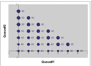
IV. NUMERICAL EXAMPLE

Let the arrival rate to the two-stage serial manufacturing

systembe A = 17 while the service rate sets and respective

costs ofoperation for both stages are {30, 50, 70} 4,c 1(50) = 7,c {40, 60, 90} 2,c 2(60) = 6,c

1(70)

= 12 aL) a) a 2(90) = 15

The costs of holding (i,j) inventory is

bi(i) = 3i,b 2(j) = 5j

The optimal process rates obtainedby the Genetic Algorithm (see in [13]) are shown inFigure 3 for the first serverand in

Figure 4 for the second server:

I Be

5c @0s

411 @0 @0

1 2

Queue#1

Fig. 3. Optimalprocessratesforserver1

V. CONCLUSION

In this study, we modeled a stochastic two-stage

manufac-turing system with two M/M/1 queueing systems in series. The controllable process rates for both stations took values

from finite sets. For the case where the single step costs

associated with the process rates and the inventory levels are

non-decreasing convex, we show that there exist threshold

policies on both inventory levels for selecting the optimal process rates.

Extendingthese results for the N-machine seriesproduction

line is the subject ofongoing research.

Queue#1

Fig. 4. Optimalprocessratesforserver2

[4] M. S. Branicky, V. S.Borkar, and S. K. Mitter, "A unified framework forhybrid control: Model and optimal control theory," IEEE Tr on

Automatic Control, vol. 43,no. 1,pp.31-45, 1998.

[5] R. L. Grossman, A.Nerode, A. P. Ravn, and H. Rischel, eds., Hybrid Systems - Vol. 736 of LectureNotes in Computer Science.

Springer-Verlag, 1993.

[6] Y. Wardi, C. G. Cassandras, and D. L. Pepyne,"Abackwardalgorithm forcomputing optimal controls for single-stage hybrid manufacturing systems," Int. J. Prod. Res., vol. 39-2,pp.369-393, 2001.

[7] C. G. Cassandras and K.Gokbayrak, "Optimalcontrol for discrete event andhybrid systems,"Modeling, Control and Optimization of Complex Systems,pp. 285-304, 2002.

[8] Y. C. Cho, C. G.Cassandras, and D. L. Pepyne, "Forward decomposition algorithms for optimal control ofaclass ofhybrid systems," Intl. J. of Robust and NonlinearControl, vol. 11,pp. 497-513, 2001.

[9] C. G. Cassandras, D. L.Pepyne, and Y. Wardi, "Optimal control ofa

class ofhybrid systems,"IEEE Trans. onAutomaticControl, vol.

AC-46,3,pp. 398-415, 2001.

[10] K. Gokbayrak and C. G. Cassandras, "Stochastic optimal control ofa

hybrid manufacturingsystemmodel," Proc. of38thIEEEConf Decision andControl,pp. 919-924, 1999.

[11] D. P. Bertsekas, DynamicProgramming and Optimal Control. Belmont, Massachusetts: AthenaScientific, 1995.

[12] 0. Selvi and K.Gokbayrak, "Stochastic optimal control ofatwo-stage

hybrid manufacturing system," Tech. Rep.2005-01, Bilkent University, IndustrialEngineeringDepartment, 2005.

[13] M. Mitchell, An Introduction to GeneticAlgorithms. TheMIT Press, 1998.

REFERENCES

[1] C. G. Cassandras and S. Lafortune, Introduction to Discrete Event Systems. KluwerAcademicPublishers, 1999.

[2] A. Alur, T. A. Henzinger, and E. D. Sontag, eds., Hybrid Systems. Springer-Verlag, 1996.

[3] P. Antsaklis, W. Kohn, M. Lemmon, A. Nerode, and S. Sastry, eds., Hybrid Systems. Springer-Verlag, 1998.

U1

cl

(30)

U2 c2(40)