328 IEEE TRANSACTIONS ON ROBOTICS AND AUTOMATION, VOL. 11, NO. 3, JUNE 1995
Inertial Navigation Systems
for Mobile Robots
Billur Barshan and Hugh
F.
Durrant-Whyte, Member, ZEEEAbstract- A low-cost solid-state inertial navigation system (INS) for mobile robotics applications is described. Error models
for the inertial sensors are generated and included in an Extended Kalman Filter (EKF) for estimating the position and orientation of a moving robot vehicle. Two Merent solid-state gyroscopes have been evaluated for estimating the orientation of the robot.
Performance of the gyroscopes with error models is compared to the performance when the error models are excluded from the system. The results demonstrate that without error compensation, the error in orientation is between 5-15"/min but can be improved at least by a factor of 5 if an adequate error model is supplied.
S i a r error models have been developed for each axis of a solid-state triaxial accelerometer and for a conducting-bubble tilt sensor which may also be used as a low-cost accelerometer. Linear position estimation with information from accelerometers and tilt sensors is more susceptible to errors due to the double integration process involved in estimating position. With the system described here, the position drift rate is 1-8 c d s , depending on the fre- quency of acceleration changes. An integrated inertial platform consisting of three gyroscopes, a triaxial accelerometer and two tilt sensors is described. Results from tests of this platform on a large outdoor mobile robot system are described and compared to the results obtained from the robot's own radar-based guidance system. Like all inertial systems, the platform requires additional information from some absolute position-sensing mechanism to overcome long-term drift. However, the results show that with
careful and detailed modeling of error sources, low-cost inertial sensing systems can provide valuable orientation and position information particularly for outdoor mobile robot applications.
I. INTRODUCTION
NERTIAL navigation systems are self-contained, nonra-
I
diating, nonjammable, dead-reckoning navigation systems which provide dynamic information through direct measure- ments. In most cases an INS must be integrated with other absolute location-sensing mechanisms to provide useful infor- mation about vehicle position. Models that describe the outputs of inertial sensors sufficiently accurately are essential if the in- formation is to be used effectively. Fundamentally, gyroscopes provide angular rate information, and accelerometers provide velocity rate information. Although the rate information is reliable over long periods of time, it must be integrated to provide absolute measurements of orientation, position and velocity. Thus, even very small errors in the rate information Manuscript received August 6, 1993; revised October 6, 1994. This work constitutes part of the OxNav project supported by SERC-ACME grant GRl638375.B. Barshan is with the Department of Electrical Engineering, Bilkent University, Bilkent, 06533 Ankara, Turkey.
H. F. Durrant-Whyte is with the Robotics Research Group, Department
of Engineering Science, University of Oxford, Oxford, OX1 3PJ United Kingdom.
IEEE Log Number 9409082.
provided by inertial sensors cause an unbounded growth in the error of integrated measurements. As a consequence, an
INS
by itself is characterized by position errors that grow with time and distance. One way of overcoming this problem is to periodically reset inertial sensors with other absolute sens- ing mechanisms and so eliminate this accumulated error. In robotics applications, a number of systems have been described which use some form of absolute sensing mechanisms for guidance (see [l] or [2] for surveys). Such systems typically
rely on the availability of easy-to-see beacons or landmarks, using simple encoder information to predict vehicle location between sensing locations. This works well when the density of beacons or landmarks is high and the ground over which the vehicle travels is relatively smooth. In cases where the beacon density is sparse or the ground is uneven, such systems can easily lose position track. This is particularly a problem for vehicles operating in outdoor environments. Inertial naviga- tion systems can potentially overcome this problem. Inertial information can be used to generate estimates of position over significant periods of time independent of landmark visibility and of the validity of encoder information. Clearly, positions derived from inertial information must occasionally be realigned using landmark information, but a system that combines both inertial and landmark sensing can cope with substantially lower landmark density and can also deal with terrain where encoder information has limited value.
Inertial navigation systems have been widely used in aerospace applications [l], [3], [4] but have yet to be seriously exploited in robotics applications where they have considerable potential. In [ 5 ] , the integration of inertial and visual information is investigated. Methods of extracting the motion and orientation of the robotic system from inertial information are derived theoretically but not directly implemented in a real system. In [6], inertial sensors are
used to estimate the attitude of a mobile robot. With the classical three-gyro, two-accelerometer configuration, experiments are performed to estimate the roll and pitch of the robot when one wheel climbs onto a plank using a small inclined plane. One reason that inertial systems are widely used in aerospace applications but not in robotics applications is simply that high-quality aerospace inertial systems are comparatively too expensive for the budgets of most robotics systems. However, low-cost solid-state inertial systems, motivated by the needs of the automotive industry, are increasingly being made commercially available. Although a considerable improvement on past systems, they clearly provide substantially less accurate position information than equivalent aerospace systems. However, as we describe in 1042-296X/95$04.00 0 1995 IEEE
BARSHAN AND DURRANT-WHYTE: INERTIAL NAVIGATION SYSTEMS FOR MOBILE ROBOTS
~
329
this paper, such systems are at a point that, by developing reasonably detailed models of the inertial platform, these sensors can provide valuable information in many robot positioning tasks.
Another system which is potentially of great value for vehicle localization is the global positioning system (GPS)
[7]. GPS is a satellite-based radio navigation system that
allows a user with the proper equipment access to useful and accurate positioning information anywhere on the globe. The fact that an absolute identification signal, rather than a direct measurement of range or bearing, is used to compute location means that measurements are largely independent of local distortion effects. The position accuracy that can be achieved with GPS is 5 m in the military band, and 50
m in the civilian band. However using a technique known as differential GPS, in which a separate base receiver is employed, civilian accuracy may be improved to 5 m. Al- though this is not as good as can be achieved using high frequency radar, it may still be adequate for some applications. It is also worth noting that the cost of GPS receivers is remarkably low (about $1000). In [8], integration of GPS with INS is described for precision navigation in aerospace applications.
The primary motivation for the work reported in this paper has been the need to develop a system capable of providing low-cost, high-precision, short time-duration position informa- tion for large outdoor automated vehicles. In particular, the interest has been in obtaining location information for short periods when the vehicle is not in contact with any beacon or landmark information. The vehicle has pneumatic tires but no suspension and runs over a road surface at speeds of up to 6
m/s. Variations in wheel radius, tire slip and body deflection cause the encoder information to be unreliable for location estimation except over very short sample intervals. Inertial sensing offers a potential solution to this type of problem.
To make best use of low-cost inertial sensing systems, it is important that a detailed understanding of the mechanisms causing drift error are understood and a model for these derived. The approach taken in this paper is to incorporate in the system a priori information about the error characteristics of the inertial sensors and to use this directly in an extended Kalman filter ( E W ) to estimate position before supplement- ing the INS with absolute sensing mechanisms. In Section 11, a hardware implementation of a robotic INS employing three solid-state gyroscopes, a solid-state triaxial accelerom- eter and two conducting-bubble tilt sensors is described. In Section 111, the error models for each of these sensors is developed, testing them for adequacy of representation and implementing them in an EKF for error compensation. The performance of two different gyroscopes are compared in Section IV with and without an error model incorporated in the system. The adequacy of these gyroscopes are as- sessed for those robotic tasks that rely on accurate angular localization of a mobile robot. In Section V, the results of bench tests of the accelerometers when used for position estimation are discussed. Section VI describes the testing of the complete INS on a radar-guided land vehicle. Accurate vehicle position fixes from the radar guidance system in a
dense beacon environment are compared against position and orientation information predicted by the INS. In conclusion, the usefulness of low-cost INS in robotics applications, is discussed for outdoor vehicles and also for indoor guidance systems.
II.
DESCRIPTION OF INS COMPONENTSA fundamental requirement for an autonomous mobile robot is the ability to localize itself with respect to the environment. The INS system described in this paper comprises three
solid-state rate gyroscopes, a triaxial linear accelerometer manufactured by ENTRAN Devices Ltd., and two Electrolevel inclinometers (or tilt sensors) by TILT Measurement Ltd., all pictured in Fig. 1.
Gyroscope
Two different types of gyroscopes have been considered and evaluated: the Solid STate Angular Rate Transducer (START) gyroscope manufactured by GEC Avionics and the ENV-05s Gyrostar manufactured by Murata [9]. The START gyroscope is an inertial sensor originally intended for the guided munition market in the 1980’s but which has also proved to be very suitable for the vehicle control market [lo], [l 11. The device consists of a small cylinder with integral piezoelectric trans- ducers and an integrated-circuit module [12]. The principle of operation is to measure the Coriolis acceleration caused by angular rotation of a vibrating cylinder, chosen for its symmetry, around the principal axis. The cylinder is open at one end and supported on a base at the other end. Eight piezoelectric transducers are attached symmetrically around the open end of the cylinder for driving, controlling and measuring the vibrations via the integrated circuit module [13].
The Gyrostar is a small relatively inexpensive piezoelectric gyro originally developed for the automobile market and active suspension systems [9]. The main application of the Gyrostar has been in helping car navigation systems to keep track of turns for short durations when the vehicle is out of contact with reference points derived from the additional sensors. The principle of operation is very similar to that of START but the geometry is radically different: It consists of a triangular prism made of a special substance called “Elinvar,” on each vertical face of which a piezoelectric transducer is placed. Excitation of one transducer at about 8 kHz, perpendicular to its face, causes vibrations to be picked up by the other two transducers. If the sensor remains still, or moves in a straight line, the signals produced by the pick-up transducers are exactly equal. If the prism is rotated around its principal axis, Coriolis forces in proportion to the rate of rotation are created.
Both gyroscopes generate voltage outputs proportional to the angular velocity of the vehicle around the principal axis of the device. The maximum rate that can be measured with the particular START gyro under investigation is f200”/s within its linear range. The corresponding value is f90°/s for the Gyrostar. If the input rate goes beyond the maximum limits, the rate and orientation information become erroneous and need to be reset.
330 IEEE TRANSACTIONS ON ROBOTICS AND AUTOMATION, VOL. 1 I , NO. 3, JUNE 1995
Fig. 1.
accelerometer by ENTRAN Devices Ltd. (d) The Electrolevel-ELH46 inclinometer manufactured by TILT Measurement Ltd.
(a) The START gyro manufactured by GEC Avionics. (b) The ENV-05s Gyrostar manufactured by Murata. (c) The EGCX3-A linear triaxial
Accelerometer
The accelerometer measures the linear acceleration of the robot along three mutually orthogonal axes on the robot frame. The measured value naturally incorporates the gravity vector that needs to be compensated for. The maximum range of the accelerometer along each axis is f 2 g = 19.62 d s 2 . The output corresponding to each axis is a voltage proportional to the projection of the total acceleration along its direction. Each axis of the accelerometer employs a Wheatstone bridge consisting of semiconductor strain gages bonded to a simple cantilever beam and endloaded with a seismic mass. Under acceleration, the bending moment creates a strain resulting in a bridge imbalance. Consequently, a voltage proportional to acceleration is generated. The device is centrally mounted on the vehicle such that its x and y axes are level with the vehicle platform and the z axis is orthogonal.
Rlt Sensors
Two orthogonally mounted tilt sensors measure small devi- ations of the vehicle platform up to f l O o from the horizontal
x
- y plane with a discrimination of 1. The Electrolevel tilt sensor is a gravity-sensing angle transducer based on the principle of the spirit level. A suitably curved tube contains an electrically conducting liquid, three electrodes, and a gas bubble. Under the influence of gravity, the bubble floats to the highest point in the tube. As the tube is tilted, the position of the bubble relative to the electrodes changes, causing a difference in electrical resistance between electrodes. The frequency response characteristics of the sensor extends from zero to a natural frequency of 2.5 Hz.The tilt information provided by these sensors is supplied to the accelerometer to cancel the gravity component projecting on each axis of the accelerometer. Unfortunately, this infor-
BARSHAN AND DURRANT-WHYTE: INERTIAL NAVIGATION SYSTEMS FOR MOBILE ROBOTS A A LISA 11-C _ _ _ . _ _ . _ _ _ . _ _ _ _ _ _ _ _ . _ _ . . _ _ _ _ . . - - - - 331 IO M BlTslsFC S F R M
mation is only useful when the vehicle is stationary since tilt sensors are inherently sensitive to acceleration as well. When the sensor is subject to an acceleration a in a direction normal to its measuring axis in the horizontal plane, the resultant of this acceleration and the acceleration due to gravity g determines the position of the bubble. If the sensor is also tilted from the horizontal by a, the measured effective angle is
1 aeff = a
+
tan-l?.9
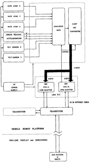
1 The block diagram for the hardware implementation of the
inertial sensors is shown in Fig. 2. The outputs of the inertial sensors are multiplexed and fed to a 12-bit A/D converter. The
digitized output is interfaced to an INMOS-T805 transputer.
The total cost of this inertial package is approximately f 5000
which is substantially less than the typical cost of inertial systems used in aerospace applications.
A
MOBILE ROBOT PLATFQKM
rv
111. ERROR MODELLING OF INERTIAL SENSORS Constructing Error Models
Building error models for inertial sensors is motivated by an attempt to reduce the effect of unbounded position and orientation errors. Dependmg on how successful these models are, inertial sensors may possibly be used in an unaided mode or for longer durations on their own. The error characteristics that dominate the operation of the INS depend on the type of inertial sensors involved. The gyroscope drift in its various manifestations is the most important contributor to navigation system errors, and is mainly dependent upon the device technology. A detailed treatment of modeling aerospace
INS'S can be found in the first volume by Maybeck [14].
For a robotic INS, the scale, nature and parameters of the localization problem are different than in aerospace. Hence, INS's developed for aerospace applications cannot be directly implemented on mobile ground vehicles. In addition, systems developed for aerospace are far too expensive to be used in robotics applications.
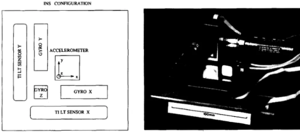
Fig. 3 illustrates the configuration of the
INS
package. The accelerometer is mounted centrally on the INS plate, and the tilt sensors are mounted along the z and y axes of the robot frame. The location of the gyroscopes are insignificant as long as they are orthogonal sincethe measured angular rate is independent of the chosen coordinate frame.To develop error models for the two types of gyroscopes,
their outputs were recorded over long periods of time when subjected to zero input, i.e. the gyroscopes were stationary on the laboratory bench. The result of this experiment over a period of 12 hours is shown in Figures 4(a) and (b) for
START and Gyrostar, respectively. Ideally, the output for
zero input would be a constant voltage level corresponding to the digital output of 2 048 for a 12-bit A/D converter as shown by the thick, solid horizontal line in the figures. The standard deviation of the output fluctuations is approximately 0.16'/s for the START and 0.24"/s for the Gyrostar. For
both gyroscopes, the real output data is at a lower level
TlLT SENSOR Y , I _ ..._..._..._..---
t
.I
.-.. !BIT M N E R mI-
. -. . -. . . 1 2 B m--.
7 1
Fig. 2. Hardware implementation of the INS.
than ideal at start-up, and the mean value gradually increases with time in an exponential fashion. Repeatability of these results indicates that an apparently small time-varying bias is characteristic of these gyros. The time variation of the bias is attributed to thermal effects based on the observation that the gyroscope units gradually heat up during operation. The bias can taper off to a negative or positive value depending on the ambient temperature. The results indicate that the Gyrostar reaches its steady state much faster than the START. Drift
in the rate output of Gyrostar is about 30 mV (1.35'/s) 10 min. after switching on and, provided there is no temperature change, about a further 10 mV (0.45'/s) during the next 24
hours [9].
The same experiment to assess the drift has also been performed for each axis of the accelerometer and for the two tilt sensors. The error characteristics of the accelerometer axes are of similar form but with differing parameters. The z axis data has been shown in Fig. 5 as an example. The error at the voltage output of each axis is characterized by a large negative bias that drifts over time. For the tilt sensors, the
332 IEEE TRANSACTIONS ON ROBOTICS AND AUTOMATION, VOL. 11, NO. 3, JUNE 1995
INS CONFIGURATION
ACCELEROMETER
TI LT SENSOR X
I
I
Fig. 3. Geometric configuration of the INS.
A/D output = 2048
($
+ 1)t
I
I
ideal output parameter fit CI*(l - e - * ) + c,, mu , time(hours) 0 2 4 6 8 10 I2 A/D output = 2048(9
+ 1)'
idealoutput 0 OeI.' I
output does not exhibit any drift, obviating the need to build an error model [ 151. The dominating source of error for the tilt sensors is the input-output nonlinearity for angles between
A/D output = 2048
(e
+
1)2sm I time(hours)
0 2 4 6 8 IO 12
Fig. 5. Digitized output of the I axis of the ENTRAN accelerometer shown along with the fitted model of form Cl(1 - e-
f
)+
Cz . Data was collected over a period of 12 hours by sampling every minute when the z axis was subject to gravity.f5-10'. The calibration data provided by the manufacturer is used to model this effect.
In the following, let
~ ( t )
be the bias error associated with measuring the true value of a quantity of interest using inertial sensors. A nonlinear parametric model of the following form was fitted to the data from the gyroscopes and the accelerometer using the Levenberg-Marquardt iterative least- squares fit method [16]:where E model(t) is the fitted error model to the gyroscope output when zero input was applied, with parameters CI, C2,
and
T
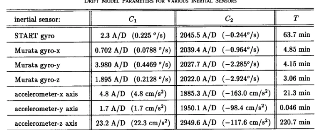
to be tuned. Starting with reasonable initial guesses for the parameters, convergence to a local minimum is achieved within 5-10 iterations. The best fitting parameter values to the experimental data are tabulated in Table I for the inertial sensors which comply with this model. Note that the z axis of the accelerometer is subject to gravity when no other acceleration is applied to the sensor. Since the tilt sensors do not exhibit this type of drift error, they are not included in the table.BARSHAN AND DURRANT-WHYTE INERTIAL NAVIGATION SYSTEMS FOR MOBILE ROBOTS 333 TABLE I
DRIFT MODEL PARAMETERS FOR VARIOUS h X T L 4 L SENSORS
Testing Adequacy of Error Models
In general, a model fitted to experimental data is regarded as being adequate if the residuals from the fitted model constitute a white, zero-mean process. Hence, one can start with any reasonable model based on inspecting the original data and test its residuals for whiteness. If the test fails, the model can be further developed until the residuals pass the whiteness test. This implies that the test for the validity of any model is basically reduced to a test for whiteness.
Following this route, the sufficiency of the above model in (2) is determined for each sensor by applying a whiteness test to the residuals in the autocorrelation domain. For a discrete system with sampling interval T,, the residual w ( k ) at time kT, is computed as follows:
Since the trend in the data has been subtracted out, the process w ( k ) is assumed to be stationary, in which case the autocovariance R,, becomes only a function of the lag A
between two data samples. When only a finite set of N data samples is available for estimation, the expressions for the sample biased autocovariance estimate is given by [17]:
(4) 1 N - l A l - l
&,(A) = -
N k = O w ( k ) w ( k
+
A ) .Ideally, the autocorrelation function of a zero-mean white process is a spike for zero lag (A = 0), corresponding to the process variance, and zero otherwise. With a finite and fixed number of data points, the sample autocorrelation will have some fluctuations around the ideal that need to be tested for statistical significance. If N is sufficiently large (N >16), it can be shown that [18] the distribution of the sample
autocovariance estimate for nonzero A is well approximated by a Gaussian distribution with zero mean and standard error given by: 1.0 0.8 0.6 0.4 0.2 0.0
Fig. 6. Biased sample autocorrelation estimate of the residuals. The result was obtained by an ensemble average over the autocorrelations of 10 data
sequences, each of 10 s duration. The dotted lines indicate
~e
f a - and M R w w ( 0)f 2 B R
bounds for the autocorrelation estimate.
In Fig. 6, the sample autocorrelation estimate, i.e. sam-
ple autocovariance estimate scaled by the estimated process variance R,,(O), is shown for the START gyroscope. An
ensemble average over the autocorrelation estimates of M = 10 data sequences (each of 10 s duration) was taken, reducing
the standard error bounds by
&.
The dotted lines corre-b - 2bR
spond to the
f
mFw
(o) andf
m r i ~ ; ( o ) bounds for the autocorrelation estim2;. These bounds determine the standard error for estimating the autocorrelation of a white process, given the finite and fixed amount of data [19]. Since thesample autocorrelation error distribution of a white process is Gaussian the autocorrelation estimate is bound to lie withinfmEiww(o) 2AR 95.5% of the time. In compliance, the
~
334 IEEE TRANSACTIONS ON ROBOTICS AND AUTOMATION, VOL. 1 I , NO. 3, JUNE 1995
25R
results indicate that the estimate is within
f
w w about96% of the time.
The positive outcome of the whiteness test on the model residuals demonstrates that the model in (2) adequately repre- sents the slowly varying bias error on the rate output of the START gyroscope. The same whiteness test has been applied to the residuals of the model for the Gyrostar and each axis of the accelerometer. The results have proven to be positive but are not included here for brevity. In the next section, the error models developed are exploited in an EKF to compensate for the errors.
d m R W W ( O )
Implementation of the Error Models
represented by the following differential equation:
The parametrized model of (2) for the bias error can be
with initial conditions ~ ( 0 ) = C2 and i(0) = $$. After
discretization, (6) becomes
E(k
+
1) = -5- E(k)+
-
I s (Cl+C2)T
+
T, T+
T, withE(0) = (7.2. (7) Due to its recursive nature, this difference equation is inde- pendent of start-up time but relies on a good estimate of the initial bias.
The quantities observed by the INS incorporate the bias errors described by (7). The observations are the rate outputs of the gyros, acceleration components on the robot frame and the two tilt measurements, leading to the nonlinear observation equations shown at the bottom of this page. Here, a,, ay and g are the accelerations of the robot in the world coordinate frame, related to the measured accelerations by a rotational transfor- mation through the Euler angles [20] 0,
4,
'P around z, y and z axes, respectively. The observations ZG, ( k ) , ZG, ( k ) , ZG, ( k ) ,Z A , ( ~ ) , ZA,(~) and z ~ , ( k ) , are, respectively, of the Euler
angle rates j ( k ) ,
q ( k ) ,
& ( k ) , and the accelerations u , ( k ) , uy(k), a Z ( k ) along the z, y, andz
axes. Each observation is taken in additive drift ~ e ( k ) , ~ $ ( k ) , € & ( I C ) , ~ ~ ~ ( k ) , c a V ( k ) , e g ( k ) , each independently modeled by (7), and additive white noise wl(k), w2(k), w3(k), wq(k), 215(k), wg(k), respectively.Note that the tilt sensor outputs are not directly supplied as observations to the filter. Since the tilt sensors provide more accurate angular information than the gyroscopes when the robot is not accelerating, the gyros are reset by the outputs of these sensors whenever the absolute value of all the accelera- tion components are less than a prefixed threshold whose value is determined by the noise level of the accelerometer output. The tilt sensors do not directly measure the Euler angles but the inclination with respect to the horizontal plane, whereas the integrated output of the gyroscopes correspond to the actual rotations around each axis on the robot frame. Suppose CY, and
ay are the angles with the horizontal plane measured by the tilt sensors lying along z and y axes, respectively. From simple geometry, these are related to the Euler angles as follows:
8 = C Y ,
q = Qy,
cos a,
Equations (7) can be rewritten in matrix notation as
z ( k ) =
h[x(k)]
+
v(k) (1 1)where
x(k)
is the state vector as described below and v(k) isa white measurement noise process vector.
Given the observations, the states that need to be estimated are the true values of orientation, angular rate, linear accelera- tion, velocity, position and the errors associated with them. Hence, the states of interest are augmented by (7) for the sensors involved, to estimate and compensate for the time- varying bias errors. The resulting state equations of the EKF
k)laz(k)
+
[sin 0 ( k ) . sin $(IC). sin @ ( k )+
cos 0 ( k ) . cos @ ( k ) ] a ,(k)
+
sinO(k).cos$(k).g(k)+
c a , ( k )+
w5(k)= [cos
e(
k ) . sin $( k ) . cos 'P( k )+
sin 0 ( k ) . sin 'P( k ) ] a , (k)+
[cos 0(k)
.
sin $ ( I C ) . sin 'P(k)
-
sine(
k).
cosa(
k)]ay ( k )2.4, (IC)
BARSHAN AND DURRANT-WHYTE INERTIAL NAVIGATION SYSTEMS FOR MOBILE ROBOTS X G , (IC
+
1 )-
XG,( k
+
1 ) X G Z ( I C f l) XA, ( I C+
1 ) XA,( k
+
1 ) - x A , ( I C+
1 ) - =LUA,
J -FG= 0 0 0 0 0 O F G , O 0 0 0 0 O F G , O 0 0 0 0 O F A , O 0 0 0 0 O F A , O - 0 0 0 0 0 FA, with O T . -20 -40 -60 -80 and - \ - '7, 1 -\\:
'k \ \\ \ -.
" " " " ' - 335 0.5 0.0 -0.5The remaining block matrices FG,, FG, , FA,,
FA^,
and block state vectors XG,, XG,, XA,, XA, in (12) have very similardefinitions to those in (13) and (14) but with the corresponding error model parameters substituted in. The overall state vector comprises 30 states. More compactly, (12) can be rewritten as (13)
Note that the state transition is linear unlike the nonlinear measurements described by (1 1). The first four states are the true values of the orientation and its derivatives, and the next two states constitute the error model for the gyroscope. This part of the filter has a constant (a
(k)
structure augmented by the error model. Lower-order filters have been implemented but shown to have a delay and much ringing in their unit- step response. With this higher-order model, the filter is able to track abrupt changes in angular velocity very closely as will be shown in the next section. The remaining states of the filter correspond to the true values of position, velocity and acceleration in the world frame, plus the error states for measuring acceleration. One interesting point to note is that for each different sensor, the error states are coupled to their relevant true states only through the observation equations and not by the structure of the state transition matrix F.In setting the process noise covariance matrix Q for the
EKF, a continuous-time white-noise model is assumed as described in [21]. With this assumption for each independent sensor block, the following process noise covariance matrix (14)
20 0 -20 -40
'
0 1 2 3 4 5 time(min) (a) -40'
I 0 1 2 3 4 5 time(min)IEEE TRANSACTIONS ON ROBOTICS AND AUTOMATION, VOL. 11, NO. 3, JUNE 1995
500 0 -500 -1000 0 1 2 3 4 5 -1500 time(min) (b) W e d 0 -20 -40 -60 -80 -100 0 1 2 3 4 5 time(min) (d)
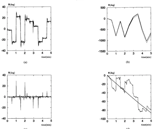
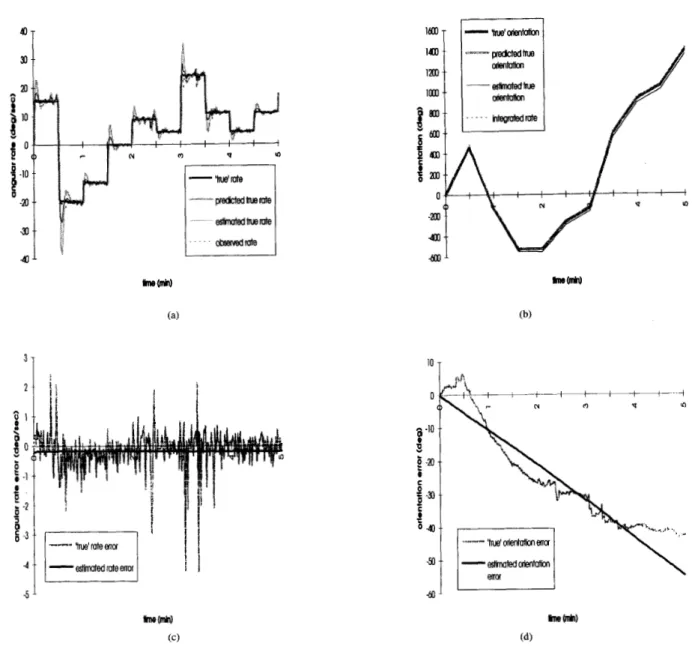
Fig. 8. (a) Angular rate; and (h) position of the START gyroscope when nonzero input is applied. A new angular rate was randomly generated every
30 s and applied to the gyro. The true values (thin, solid lines) and the erroneous Observations (dotted lines) are displayed along with the EKF results (thick, solid lines) which compensate for the error. (c) Error in the angular rate and (d) error in orientation. Both the true (thin, solid lines) and the estimated values (heavy, solid lines) are shown.
can be derived: 0 0 0 0
[Y
QG 0 0 0X 1
withl
o
0 0 andwhere u1 = 0.05"/s3,u2 = 0.2"/s, u3 = 3 cm/s2, and 0 4 =
0.01 cm/s2, with u2, u4 being the experimentally determined standard deviations of the residuals from the fitted models.
The state vector estimated by the filter is given by the standard recursive estimator
x ( k
+
Ilk+
1) = FX(k(k) + U+
W(k+
l ) v ( k+
1) (18) wherex(k
+
llk
+
1) is the estimate made of the state vector at time ( k+
l)Ts based on all observations up to this time,x(klk)
is the estimate at the previous time-step, W(k+
1) is the filter gain, and v(k+
1) = z(k+
1) - h[x(k+
ilk)]is the innovations vector provided by the new observations at time ( k
+
l)T,. A detailed treatment of EKF prediction and update equations can be found in [21]. An important point to note is that all states, including drift parameters, are estimated at every sample time.The EKF structure in (11) and (16) has been implemented in real time on an INh4OS-T805 transputer network where a minimum sampling interval of T, = 30 ms is achieved. Each gyroscope has been mounted on a rotating platform whose angular velocity and orientation can be accurately controlled and measured. An HCTL-1100 chip was used to control the motor in the integral velocity mode. The motor position from the encoder is accurate to 1/2000 of a revolution. A 500-line optical encoder was used to measure motor position, driving
BARSHAN AND DURRANT-WHYTE INERTIAL NAVIGATION SYSTEMS FOR MOBILE ROBOTS
the platform through a low backlash 20:l gearbox. The most significant positioning error is in gearbox backlash. This is very good, however, and better than 1/10 of a degree. For comparison purposes, the platform velocity and orientation are taken to be the "true" values of these quantities in the next section. Initial estimates of the bias errors are made to initialize the filter by averaging the output of each inertial sensor over a large number of samples when the robot is not in motion. Since the start time of the experiment can correspond to any point on the curves in Figs. 4 and 5, it is important to have good estimates of the initial biases. For an initial estimate with over 1 000 samples from each sensor, data collection and estimation take only 1-2 s on an INMOS-T805 transputer network hosted by an IBM-80486 PC. As data is collected by the inertial sensors, the parallel-running EKF filters the measurements and provides estimates of the quantities of interest for the mobile robot.
Iv. COMPARISON OF TWO SOLID-STATE GYROSCOPES To determine the adequacy of the error models, the system performance with no assumed error model is compared to the performance when the error models summarized in Table I are incorporated in the EKF for each gyroscope.
Performance of START
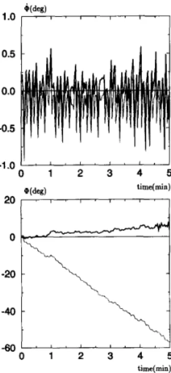
The results when zero input was applied to the START gyroscope are shown in Fig. 7 over a duration of five minutes. The true values and the erroneous observations are illustrated along with the EKF output which compensates for the error. In this experiment, the system was close to start-up, and the bias error had negative values. At the end of the experiment, the integrated gyroscope rate output exhibited an error of -70.8"/s, whereas the compensated and filtered output was
+8.6', having had an overall maximum deviation of +12.0°
from the true value. Similar experiments indicate that the typical improvement factor is approximately 6.
Fig. 8 illustrates the angular rate and position of the START gyroscope when nonzero input was applied for a total duration of five minutes. A new angular rate -25
5
5
25'/s was randomly generated every 30 s and applied to the gyro. The true values and the erroneous observations are displayed along with the filter results. Note that the drift in the orientation is more significant than in the angular rate since even very small errors quickly accumulate when integrated. To make this more visible, the true and estimated errors in rate and orientation are shown separately in Fig. 8(c) and (d) for the same data. At the end of the experiment, the integrated rate output was erroneous by -84.7" (the worst case) whereas the filtered estimate had an error of +3.4', indicating that the filter slightly overcompensated for the bias in this particular case. During the course of the experiment, however, the compensation was not always as good, the worst-case error being 36.0', due to the large spiky errors in the measured angular rate at those points when a new rate was suddenly applied to the gyro.These errors can be seen in Fig. 8(d) more clearly. Both the gyroscope rate output and the filtered rate output were accurate within f 2 S 0 / s at the end of the experiment.
337 - 1 . 0 ' ' ' ' ' ' ' ' ' '
'
0 1 2 3 4 5 time(min) W e d 1 -20 O P T V" 0 1 2 3 4 5 time(min)Fig. 9. Angular rate (top) and orientation (bottom) for the zero-input case of the Murata gyro when the bias error is negative. The true values (thin, solid line) and the erroneous observations (dotted line) are illustrated along with the EKF output (heavy, solid line) which compensates for the error.
P e g o m m e of Gyrostar
The results when zero-input was applied to the Gyrostar are shown in Fig. 9 over a duration of five minutes. At the beginning, the system was close to start-up and the bias error had negative values. At the end of the experiment, the integrated gyroscope rate output exhibited an error of -95.9"/s, whereas the compensated and filtered output was -0.21", having had an overall maximum deviation of -3.8' from the true value. The typical improvement factor was approximately 8.
Fig. 10 illustrates the angular rate and position of the
Gyrostar when nonzero input was applied for a total dura!ion of five minutes. As before, a new angular rate -25
5
5
25'/s is randomly generated every 30 s and applied to the gyro.
The true values and the erroneous observations are displayed along with the filter results. The true and estimated errors in rate and orientation are shown separately in Fig. 1O(c) and (d) for the same data. At the end of the experiment, the integrated rate output exhibited an error of -42.5' whereas the filtered estimate was +10.7", indicating that the filter slightly overcompensated for the bias in this particular case. As shown in Fig. IO(d), there is a much better agreement between the estimated position error and its true value than with the START gyro. This is due to Gyrostar being more shock tolerant than the START. Both the gyroscope rate output and the filtered rate output were accurate within f1.5'/s at the end of the experiment.
338
d esfimoted rate error -5
IEEE TRANSACTIONS ON ROBOTICS AND AUTOMATION, VOL. 11, NO. 3, JUNE 1995
-1
14n
1200
IUJI
0 t
Fig. 10. (a) Angular rate and (b) position of the Gyrostar when nonzero input was applied. A new angular rate was randomly generated every 30 s and applied to the gyro. The true values and the erroneous observations are displayed along with the EKF results which compensate for the error. (c) Error in the angular rate and (d) error in orientation. Both the true and the estimated values are shown.
was selected for the robotic INS since it proved to perform better than the START in addition to being more compact, light and inexpensive.
v.
EVALUATION O F THE ACCELEROMETER To determine the adequacy of the error models for each axis, the system performance with no assumed error model is com- pared to the performance when the error models summarized in Table I are incorporated in the EKF for each axis of the accelerometer. Experiments similar to those in the previous section have been performed both for zero-input and nonzero- input case 1151. For the zero-input case, when the error model was included, the maximum error in velocity was 38 c d sin absolute value and 30 m in position after about 3 min. Even with error compensation, this example indicates how quickly small errors in the rate outputs accumulate when the rate information is integrated to obtain velocity andor position information.
To evaluate the accelerometer for position estimation when in motion (nonzero-input case), a simple experiment was designed: The robot platform was accelerated and decelerated over a distance of 30 cm along its 2 axis in the forward
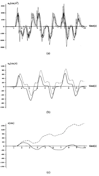
and backward directions. The results from the accelerometer are illustrated in Fig. 11. In Fig. ll(a), real data from the accelerometer is shown in dotted line, EKF estimate is in solid line. The dashed line corresponds to the output of the
BARSHAN AND DURRANT-WHYTE: INERTIAL NAVIGATION SYSTEMS FOR MOBILE ROBOTS 339 . . 60- 40- 0 - -20 - - 4 0 - -60 - zo - - 1 0 0
1
time(s) (C)Fig. 11. In (a), real data from the I axis of the accelerometer is shown in dotted line, EKF estimate is in solid line. The dashed line corresponds to the output of the tilt sensor I functioning as an accelerometer. In (b) and (c), solid lines indicate EKF estimates of velocity and position along the 2 axis. The dashed lines correspond to the numerical integration of tilt sensor output.
tilt sensor
x
functioning as an accelerometer for comparison purposes. In Figures ll(b) and (c), solid lines indicate EKF estimates of velocity and position along the z axis. The dashed lines correspond to the numerical integration of the tilt sensor output. At the end of the experiment, position estimation using the accelerometer was erroneous by -15.3 cm. Vibrations of the platform were kept at a minimum by performing the experiment on a very smooth surface. This caused.the drift on the accelerometer to be relatively small. In more realistic situations, the position estimation error can easily exceed 60-80 cm over a duration of 10 s.Linear position estimation with information from ac- celerometers and tilt sensors is more susceptible to errors due to the double integration process. With the described system, the position drift rate is between 1-8 c d s , necessitating the fusion of information from absolute position-sensing
Fig. 12. FRAIT 80 vehicle at the Firefly Ltd. test site.
mechanisms.
VI. TESTING OF THE INS ON A LAND VEHICLE The INS has undergone tests on an automated land vehicle provided by Firefly Ltd. and pictured in Fig. 12. The vehicle weighs 19 tonnes and is designed to cany I S 0 standard cargo containers up to a capacity of 80 tonnes. It is powered by diesel hydraulic drives and can achieve speeds up to 6 d s . It has a dual-Ackerman steer configuration with both front and rear wheels steering independently to allow crabbing motions. Tires are conventional pneumatic tires with no suspension. The main vehicle guidance system consists of two frequency- modulated continuous wave millimeter-wave radar systems operating at 94 GHz with a swept bandwidth of 500 MHz.
These provide range and bearing information to a set of 12 special radar reflectors placed around the test area. The range resolution is 10 cm, the bearing resolution approximately 1’ and the maximum range about 200 m. Beacon bearing and range measurements are used to compute location and velocity estimates of the vehicle with respect to a fixed beacon map. The absolute accuracy of the guidance system is approximately 3 cm over the test area. Since the information provided by the radar is very accurate and does not drift with time, this is used as an “absolute” reference to compare the accuracy of the position and orientation data provided by inertial sensors. Ultimately, the aim of the inertial system is to aid the radar- based navigation system in areas where beacon observations are infrequent, and for new vehicles travelling at substantially higher speeds where increased short-term accuracy is required. In such situations, the INS state estimator is used to provide improved short-term predictions between beacon observations which are then integrated in a subsequent navigation filter which incorporates a model of vehicle kinematics. This is known as a feedback filter configuration. This should be contrasted with a feedforward filter configuration in which the INS filter incorporates the vehicle model, and beacon observations are used to correct the estimates produced by this filter [ 141. Consequently, the experimental results described here concentrate on describing the stand-alone prediction performance of the
INS
platform.IEEE TRANSACTIONS ON ROBOTICS AND AUTOMATION, VOL. 11, NO. 3, JUNE 1995 340 150 100 50 0 , .,m -5 0 5 10 15 0 15 rim)
Fig. 13. On the left are z - y position of the FRAIT 80 vehicle as estimated by the radar for two different runs. On the right, corresponding z position of the FRAIT 80 vehicle versus time as estimated by the radar.
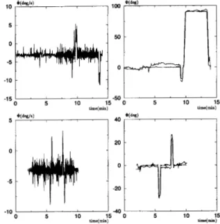
On the left-hand column of Fig. 13, the trajectory of the vehicle for two different runs is shown in the z - y coordinate frame (note the nonequal scaling of z - y axes). In both runs, the vehicle starts off at ( z i p ) = (0,20), moves along the y axis and comes backward to its starting point to continue along different trajectories. The duration of each run is different. To make the trajectories more clear, the z coordinate is illustrated on the right-hand side of the same figure as a function of time. In Fig. 14, raw angular rate data from the z gyroscope is shown for the two runs. By filtering the Gyrostar rate output with error compensation, a vehicle orientation estimate is obtained as illustrated on the right-hand side of the figure in dotted line. This result is compared to the @ estimate from the radar shown in solid line. Since the radar data is very accurate, it is taken to be the true value of the orientation for purposes of evaluation. It can be seen that the orientation estimate produced from the INS compares very well with the orientation estimate produced by the radar system. Over a run time of approximately 10 min., the maximum orientation error is of the order of 5". This is actually substantially better than
predicted from the bench tests conducted on the INS. It is conjectured that this is because the turning motions of the vehicle are not as abrupt as those generated during bench testing, and orientation estimates are generally good following these turning motions. These results indicate that the
INS
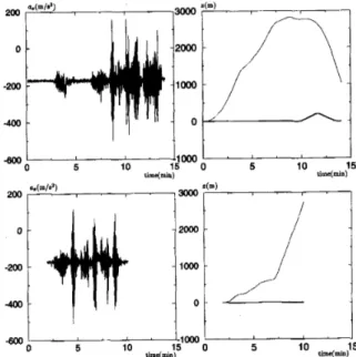
can be used to provide reliable vehicle orientation information over relatively long periods of time of the order of 10 min. and possibly longer.Fig. 15 illustrates raw data from the z axis of the ac- celerometer on the left-hand side. This data needs to be double integrated and error compensated to obtain linear position information. Using the previously described EKF structure, the corresponding result shown on the right-hand side of the same
10 time(mi 5 15 time(min) 10 -401 ' ' ' ' '
'
15 0 lo time(min)Fig. 14. On the left, Gyrostar rate output data for two different runs. On the right, corresponding orientation estimafe using the Gyrostar rate output and radar data for two different runs. The @ estimate using the radar data is shown in solid line, and the estimate obtained by filtering the gyro data is shown in dotted line.
figure is obtained. There are large discrepancies between the very accurate radar position data and the results obtained from the accelerometer over the duration of the test runs. This is due to the sensitivity of the accelerometer to very small vibrations and errors which quickly grow as a result of the double integration process. As described in the previous section, under idealized laboratory conditions, position information from the accelerometer is useful only over a duration of about 5 s.
Fig. 16 shows the error between radar position estimates and
INS
position estimates for a series of short segments of both test runs for a period of up to 25 s (the error being reset to zero at the beginning of each segment). This shows that for short durations the maximum drift rate in position estimates given by the INS is approximately 28 c d s . Thus, although the position information derived from the INS platform has substantially higher drift rates than the orientation estimates for long durations, the position information is still valuable over short time durations and can be used to improve position prediction information in a filter configuration.The nature of beacon-based navigation using some absolute sensing mechanism (like radar) requires that a good prediction of vehicle location is made at each time step so that the process of matching observed beacons to a map of beacon locations (data-association) can be done accurately and efficiently. The
INS
described in this paper provides a good means of provid- ing such predictions particularly in situations when only sparse beacon layouts are available or when the vehicle is running at high speeds over rough terrain. Error in predicted vehicle ori- entation is a notable source of difficulties in beacon matching, because of instabilities arising from nonlinearities involved in using the observation model to predict beacon location.BARSHAN AND DURRANT-WHYTE: INERTIAL NAVIGATION SYSTEMS FOR MOBILE ROBOTS
Fig. 15. On the left, raw data obtained from the z axis of the accelerometer for the two runs. On the right, corresponding I position estimate (dotted line) compared to the z position estimate from the radar (solid line) for the same two runs.
The low-drift rates associated with INS orientation estimates provides a direct means of minimizing such problems. Linear error in beacon matching is less of a problem because of the linear relationship between vehicle and beacon location errors. Thus, although the linear position predictions produced by the INS are substantially worse than the orientation estimates, they are still of considerable value in beacon-based navigation. Practically, the FRAIT-80 vehicle described observes a beacon
approximately 3 times a second to provide an accuracy of 5 cm at 6 d s . The addition of INS information will allow the same
accuracy to be achieved with a reduction in beacon observation frequency to once every 2-3 s, or a speed increase to 12-15
m l s
.
VII. DISCUSSION AND CONCLUSION
The purpose of the research described in this paper was to develop a low-cost INS system of general use in mobile robot guidance problems and specifically to aid in the navigation of high-speed outdoor vehicles. An INS comprising three solid- state gyroscopes, a triaxial accelerometer and two Electrolevel tilt sensors has been described. A detailed model of the navigation information available from these sensors has been validated. One of the most important results in this paper is that by developing a careful and accurate model of the INS
sensors, substantial improvements in performance can be made which make the application of low-cost INS'S to mobile robot
applications a viable proposition.
We have described a simple extended Kalman filter which takes as input the measurements made by the INS sensors and produces estimates for the platform position, orientation, their derivatives, and corresponding drift rates. This filter was used to test the INS under laboratory conditions, first
-2
-4
i
34 I
Fig. 16. y position estimate derived from the y axis of the accelerometer (in dotted tine) compared to the radar data over short durations (in solid line) for the two runs.
under zero-input conditions, and subsequently when subject to known input motions. These were used to provide preliminary estimates of position and orientation estimate errors. A number of conclusions from these tests were made, in particular, the orientation estimates obtained were reliable and useful over quite long periods of time (with the Gyrostar sensor performing best), while the position estimates obtained were reliable over shorter periods. In both cases, the drift models developed for these sensors substantially increased estimate accuracy.
The
INS
was tested on a radar-equipped land vehicle for evaluation and comparison purposes. The orientation estimates produced were found to be reliable over periods of at least 10 min., however, under field conditions where the vibrations can be large, the position estimates produced were reliable only over periods of 5-10 s. In feedforward configuration, this level of accuracy can be used to provide much improved vehicle location predictions which inturn
permit either a reduction in beacon density or an increase in vehicle speed.Objectively, the orientation information available from the INS is far better than position information. Although both are useful in outdoor applications like those described, only the gyroscope information would appear to have any value in indoor mobile robot applications. The low orientation drift rates associated with the gyroscope provide a low-cost means of obtaining good orientation information for a mobile vehicle. However it is unlikely that the accelerometer information would be any better at providing position estimates than the simple use of wheel encoders on indoor vehicles. This, though, has significant implications as it is most often the turning motions of indoor vehicles that introduce substantial position uncertainty due to the geometric magnification of orientation error into position error. Thus the use of a solid-state gyro-
342 IEEE TRANSACTIONS ON ROBOTICS AND AUTOMATION, VOL. 1 I , NO. 3, JUNE 1995
scope on indoor vehicles could yield substantially improved navigation performance, while the use of accelerometers is likely to be of only marginal value.
Our
current work is focused on three main applications of this type of sensing technology. The first is the integration of an INS unit like that described above with both radar (in terrain-aiding mode) and GPS navstar data in high-speed (60 mph) navigation systems. The second is the use of a twin- gyroscope system on indoor vehicles to estimate orientation and heading derived from the vehicle steer geometry. This has practical significance because the rate of orientation change (as measured by the gyroscope) is directly proportional to the effective steer angle of the vehicle wheels, which can con- sequently be measured without drift. Finally, we are looking at the application of this INS to low-cost underwater vehicles where only sparse navigation information is available.REFERENCES
M. M. Kuritsky and M. S. Goldstein, Eds., “Inertial navigation,” in
Autonomous Robot Vehicles, I. J. Cox and G. T. Wilfong, Eds. New
York: Springer-Verlag, 1990.
J. J. Leonard and H. F. Durrant-Whyte, Directed Sonar Navigation. Norwell, MA: Kluwer Academic Press, 1992.
C. T. Leondes, Ed., Theory and Applications of Kalman Filtering.
London: Technical Editing and Reproduction Ltd., 1970.
D. A. Mackenzie, Inventing Accuracy: A Historical Sociology of Nuclear
Missile Guidance. Cambridge, MA: MIT Press, 1990.
T. ViCville and 0. D. Faugeras, Cooperation of the Inertial and Visual
Systems (NATO AS1 Series, vol. F63). New ;York: Springer-Verlag,
1990, pp. 339-350.
J. Vaganay and M. J. Aldon, “Attitude estimation for a vehicle using inertial sensors,” in 1st IFAC Int. Workshop on Intell. Autonomous
Vehicles, 1993, pp. 89-94.
B. W. Parkinson and S. W. Gilbert, “Navstar: Global positioning system- ten years later,” Pmc. IEEE, vol. 71, no. 10, pp. 1117-1186, 1983. B. Tiemeyer and S. Vieweg, “GPS/INS integration for precision nav- igation,’’ Technical report, Institute of Flight Guidance and Control, Technical University of Braunschweig, Hans-Sommer-Str. 66 D-3300 Braunschweig, Germany, 1992.
T. Shelley and J. Barrett, “Vibrating gyro to keep cars on route,” Eureka on Campus, Eng. Materials and Design, vol. 4, p. 17, Spring 1992. D. G. Harris, “START A novel gyro for weapons guidance,” in
University of Stuttgart Gyro Symp., 1988.
D. G. Harris, “Initial trials results for image stabilisation using a rugged low noise gyroscope,” Technical Report, Guidance Systems Division, GEC Avionics, Rochester, Kent, U.K., 1992.
C. H. J. Fox, “Vibrating cylinder gyro-theory of operation and error analysis,” in University of Stuttgart Gyro Symp., 1988.
R. M. Langdon, “The vibrating cylinder gyro,” Technical Report, The Marconi Review, 1982.
P. S. Maybeck, Stochastic Models, Estimation, and Control. New York: Academic Press, 1979, vol. 1-111.
B. Barshan and H. F. Durrant-Whyte, “Inertial navigation systems for mobile robots,” Technical Report, Robotics Research Group, Oxford University, Oxford, U.K., Aug. 1993.
S. A. Teukolsky, W. H. Press, B. P. Flannery, and W. T. Vetterling,
Numerical Recipes in C. Cambridge, U.K.: Cambridge University
Press, 1988, pp. 54&547.
M. Schwartz and L. Shaw, Signal Processing: Discrete Spectral Analy-
sis, Detection, and Estimation.
R. L. Anderson, “Distribution of the serial correlation coefficient,”
Annals Math. Statist., vol. 13, pp. 1-13, Mar. 1942.
G. E. P. Box and G. M. Jenkins, Statistical Models for Forecasting and
Control.
J. J. Craig, Introduction to Robotics: Mechanics and Control. Reading,
MA: Addison-Wesley, 1989.
Y. Bar-Shalom and T. E. Fortmann, Tracking and Data Association. New York: Academic Press, 1988.
New York McGraw-Hill, 1975.
San Francisco: Holden-Day Inc., 1976.
ACKNOWLEDGMENT
The authors would like to thank GEC Avionics, Kent, U.K., for lending a prototype START gyroscope unit for evaluation purposes. Thanks are also due to Thomas P. Burke for his help with the mechanical design of the INS platform and Edward Bell of Firefly Ltd., North Devon, U.K., for his help with collecting the data on the FRAIT 80 land vehicle.
Billur Barshan received the B.S. degree in physics
and the B.S.E.E. degree in electrical engineering from Bogaziqi University, Istanbul, Turkey, and the M.S. and Ph.D. degrees in electrical engineering from Yale University, New Haven, CT in 1986, 1988, and 1991, respectively.
From 1987 to 1991 she was a research assistant at Yale University. From 1991 to 1993 she was a postdoctoral researcher at the Robotics Research Group at University of Oxford, U.K. Currently, she is an Assistant Professor at Bilkent University, Her current research interests include sensor-based robotics, sonar and Dr. Barshan is the recipient of Nakamura Prize given to the most outstand- Ankara, Turkey.
inertial navigation systems and sensor data fusion. ing paper at the IROS 1993 International Conference.
Hugh Durrant-Whyte received the B.S. (1st class) in Nuclear and Mechanical
Engineering from the University of London, England in 1983, the M.S.E. and Ph.D. degrees from the University of Pennsylvania in 1985 and 1986, respectively.
He is currently a University Lecturer in Engineering Science at the University of Oxford, U.K. His current research interests include multi-sensor systems and robotics.