USING NONLINEAR
PROGRAMMING
a thesis
submitted to the department of computer
engineering
and the institute of engineering and science
of b˙ilkent university
in partial fulfillment of the requirements
for the degree of
master of science
by
A. Sezgin Abalı
September, 2001
Assist. Prof. Dr. U˘gur G¨ud¨ukbay (Supervisor)
I certify that I have read this thesis and that in my opinion it is fully adequate, in scope and in quality, as a thesis for the degree of Master of Science.
Prof. Dr. B¨ulent ¨Ozg¨u¸c
I certify that I have read this thesis and that in my opinion it is fully adequate, in scope and in quality, as a thesis for the degree of Master of Science.
Assoc. Prof. Dr. ¨Ozg¨ur Ulusoy
Approved for the Institute of Engineering and Science:
Prof. Dr. Mehmet Baray
Director of Institute of Engineering and Science
ANIMATION OF HUMAN MOTION WITH INVERSE
KINEMATICS USING NONLINEAR PROGRAMMING
A. Sezgin Abalı
M.S. in Computer Engineering
Supervisor: Assist. Prof. Dr. U˘gur G¨ud¨ukbay September, 2001
Animation of articulated figures has always been an interesting subject of com-puter graphics due to a wide range of applications, like military, ergonomic de-sign etc. An articulated figure is usually modelled as a set of segments linked with joints. Changing the joint angles brings the articulated figure to a new posture. An animator can define the joint angles for a new posture (forward kinematics). However, it is difficult to estimate the exact joint angles needed to place the articulated figure to a predefined position. Instead of this, an animator can specify the desired position for an end-effector, and then an algo-rithm computes the joint angles needed (inverse kinematics). In this thesis, we present the implementation of an inverse kinematics algorithm using nonlinear optimization methods. This algorithm computes a potential function value be-tween the end-effector and the desired posture of the end-effector called goal. Then, it tries to minimize the value of the function. If the goal cannot be reached due to constraints then an optimum solution is found and applied by the algorithm. The user may assign priority to the joint angles by scaling ini-tial values estimated by the algorithm. In this way, the joint angles change according to the animator’s priority.
Keywords: animation, human motion, inverse kinematics, nonlinear program-ming, optimization.
DO ˘
GRUSAL OLMAYAN PROGRAMLAMA
KULLANAN TERS K˙INEMAT˙IK Y ¨
ONTEM˙IYLE
˙INSAN MODELLER˙IN˙IN AN˙IMASYONU
A. Sezgin Abalı
Bilgisayar M¨uhendisli˘gi, Y¨uksek Lisans Tez Y¨oneticisi: Yrd. Do¸c. Dr. U˘gur G¨ud¨ukbay
Eyl¨ul, 2001
Askeri uygulamalar, ergonomik tasarım gibi geni¸s uygulama alanları olan in-san modellerinin animasyonu bilgisayar grafi˘ginin en ¨onemli konularından biri olmu¸stur. Bir eklemli v¨ucut genellikle eklemlerle ba˘glanmı¸s segmanlar seti olarak modellenir. Eklem a¸cılarındaki de˘gi¸sim, v¨ucuda yeni bir duru¸s verir. Bir animat¨or, yeni bir duru¸s i¸cin eklem a¸cılarını belirleyebilir (ileri kinematik). Fakat, v¨ucudu bir pozisyona yerle¸stirmek i¸cin gerekli kesin eklem a¸cılarını tah-min etmek zordur. Bunun yerine bir animat¨or v¨ucuttaki u¸c bir nokta i¸cin is-tenen bir pozisyonu tanımlayabilir ve sonra ters kinematik algoritması v¨ucudu yerle¸stirmek i¸cin gerekli eklem a¸cılarını hesaplar. Bu tezde, insan modellerinin animasyonu i¸cin do˘grusal olmayan optimizasyon ile ters kinematik y¨onteminin ger¸cekle¸stirilmesi anlatılmaktadır. Bu y¨ontem, son-etkileyici ve hedef olarak adlandırılan son etkileyicinin istenen pozisyonu i¸cin bir potansiyel fonksiyon tanımlar. Do˘grusal olmayan optimizasyon algoritması bu fonksiyonun de˘gerini k¨u¸c¨ultmeye ¸calı¸sır. Eklem a¸cılarının ¨ust ve alt limitleri oldu˘gundan dolayı fonksiyon de˘geri sıfırlanamayabilir. Bu durumda algoritma en iyi ¸c¨oz¨umde durur (lokal optimum). Kullanıcı, eklem a¸cılarına, algoritma tarafından tah-min edilmi¸s ilk de˘gerlerinin a˘gırlıklarını de˘gi¸stirerek ¨oncelik verebilir. B¨oylece, eklem a¸cılarının animat¨or¨un ¨onceli˘gine g¨ore de˘gi¸smesi sa˘glanmaktadır.
Anahtar s¨ozc¨ukler: animasyon, insan hareketi, ters kinematik, do˘grusal ol-mayan programlama, optimizasyon.
Aileme.
I am very grateful to my supervisor, Assist. Prof. Dr. U˘gur G¨ud¨ukbay, for his invaluable support, guidance and motivation.
I also would like to thank my thesis committee members Prof. Dr. B¨ulent ¨
Ozg¨u¸c and Assoc. Prof. Dr. ¨Ozg¨ur Ulusoy for their valuable comments to improve this thesis.
I would like to mention some people who helped me during this study in different ways. I would like to thank Captain G¨ultekin Arabacı for his invaluable support who shares some parts of this research with me. I would also like to thank Captain T¨urker Yılmaz for his invaluable help on OpenGL libraries.
Finally, I cannot forget my love and my wife, Berrin Abalı. I would like to thank her for invaluable moral support and love.
1 Introduction 1
1.1 Organization of The Thesis . . . 2
2 Modelling of Articulated Bodies 3 2.1 Representing Articulated Figures . . . 3
2.1.1 Mathematical Notation . . . 3
2.1.2 Representation of Articulated Figures in Our Implemen-tation . . . 4
2.2 Data Structures . . . 6
2.3 Geometric Body Modelling . . . 10
2.3.1 Geometric Body Modelling Techniques . . . 10
2.3.2 Surface Scheme with Triangular Polygons . . . 11
3 Human Animation Techniques 13 3.1 Kinematic Methods . . . 13
3.1.1 Forward Kinematics . . . 14
3.1.2 Inverse Kinematics . . . 15
3.2.2 Inverse Dynamics . . . 17 3.3 Motion Capture . . . 18 4 Inverse Kinematics 20 4.1 Numerical Methods . . . 20 4.1.1 Linearized solutions . . . 20 4.1.2 Nonlinear Optimization . . . 22
4.2 A Combination of Analytic and Numerical Methods . . . 23
5 Implementation Details 25 5.1 Function Generator Module . . . 25
5.1.1 Potential Function Calculation . . . 29
5.1.2 Jacobian Generation . . . 31
5.1.3 Gradient Function Calculation . . . 32
5.1.4 Constraint Matrix Construction . . . 33
5.2 Nonlinear Programming Module . . . 34
6 The Nonlinear Optimization Algorithm 35 6.1 Determining an Initial Feasible Point . . . 35
6.2 Active Constraints . . . 36
6.3 Linearly Constrained Nonlinear Optimization Algorithm . . . . 37
7 Results 41
7.1 Performance Experiments . . . 43
8 Conclusion and Future Work 46 Bibliography 48 Appendix 52 A The User Interface 52 A.1 Overview . . . 52
A.2 Viewing Area . . . 52
A.3 Menu Area . . . 54
A.3.1 Navigation Block . . . 54
A.3.2 Selecting Goal Type . . . 55
A.3.3 Assigning Scalar Multiplier to the Joint Angles . . . 55
A.3.4 Visual Properties Block . . . 56
A.4 Keyboard and Mouse Usage for GUI . . . 56
2.1 Articulated figure representation. . . 5
2.2 Placement of joints on the articulated figure. . . 6
2.3 Tree-structured hierarchy of human figure. . . 7
2.4 Segment data structure . . . 7
2.5 Site data structure . . . 8
2.6 Joint data structure . . . 9
2.7 DOF data structure . . . 9
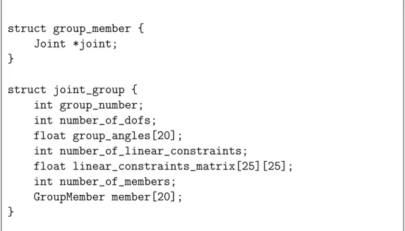
2.8 Joint group data structure . . . 10
2.9 An example file showing the 3D coordinates of points. . . 12
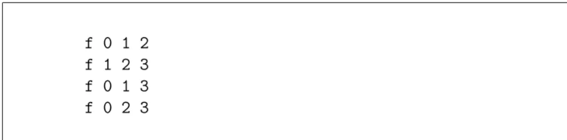
2.10 An example file that stores the polygon (face) information. . . . 12
2.11 An example shape read from files. . . 12
3.1 Given goal, more than one solution. . . 15
4.1 Iteration steps towards the desired goal. . . 21
5.1 The overall structure of the animation system. . . 26
7.1 Examples of unrealistic and realistic postures. . . 42
7.2 Examples of reachable and unreachable goals. . . 43
7.3 Example figures with and without scaling factors. . . 44
7.4 Example postures. . . 45
A.1 Graphical user interface of the system. . . 53
7.1 Average frame rates for animations . . . 43
DOF : Degrees of Freedom fps : Frames per Second
CSG : Constructive Solid Geometry SVD : Singular Value Decomposition DFP : Davidon-Fletcher-Powell algorithm
BFGS : Broyden-Fletcher-Goldfarb-Shanno algorithm
θi : ith joint angle
H : Hessian matrix
A : n-by-m constraint matrix where n denotes the number of joint angles in joint group and m
denotes the sum of all active and inactive constraints
q : The number of active constraints
aj : jth column vector of the constraint matrix
g : Gradient of the objective function as a vector
d : Search direction
G(θ) : Objective function GUI : Graphical User Interface
Introduction
Animation of articulated figures has always been an interesting subject of com-puter graphics due to a wide range of applications. In film industry, animators spend much time in order to fill the key-frames between two adjacent different positions of a figure. The usage of articulated figures in simulated environments helps the accomplishment of educational purposes and ergonomic designs. Dur-ing a presentation, an animated figure increases the understandability and the imagination of the audiences. One of the goals of computer graphics commu-nity is to model articulated figures, and to animate their actions realistically.
The level of automation in motion control of a human figure has a tradeoff between the user and the computer. On one side, the user is supposed to define all control factors for the movements of individual body parts during each time instance. In order to achieve realistic motions, the user must be highly experienced. On the other side, the user only gives a goal or a list of goals for the motion of the figure and the computer computes the parameters needed to reach the goals defined. However, the result may not be the same as what the user expects precisely.
Two basic approaches to motion control were developed. In one approach, the geometric properties of the articulated bodies are used for motion control. Positions and orientation of body segments, rotations and translations around
local and global coordinate frames are basic parameters of the approach. In-terpolations, computing the Jacobian and the gradients, optimization, etc. are helpful mathematical tools for the methods of the approach. Neglecting the physical behaviors of the objects in motion is the basic weakness of the ap-proach causing a serious loss of realism. The other apap-proach simulates the physical behavior of the objects. Newton’s laws are the fundamental princi-ple of the approach. The forces and torques for rotations are linked to the resulting motion with Newton’s equations. The approach generates realistic motions. However, the added complexity makes real time animation difficult.
One of the important issues in motion control of articulated figures is to handle the constraints. Constraints are the result of body segment limits. For example, head cannot turn back with an angle of 180-degree. While the animator gives a motion to a figure, constraints cannot be violated. Different methods have been used to handle the constraints. None of these methods is trivial.
The motivation behind this thesis is to implement an algorithm that reduces user’s job during an animation. In order to prevent undesired motions, user can also interfere with some control factors. The user will not need to take care of constraints of body parts while moving the figure reach a goal. In order to handle constraints, a constraint-based nonlinear optimization algorithm is implemented.
1.1
Organization of The Thesis
Chapter 2 explains how human figure is modelled and is represented. Chap-ter 3 reviews compuChap-ter animation techniques in general, and discusses their applicability to the concept of articulated figure animation. In Chapter 4, the inverse kinematics problem is discussed and common approaches to solving the problem are reviewed. In Chapters 5 and 6, an implementation of inverse kinematics using constraint-based nonlinear optimization is presented. Results of the implementation are presented in Chapter 7. Chapter 8 gives conclusion and future work. In Appendix A, the user interface of the system is described.
Modelling of Articulated Bodies
In this chapter, some common mathematical notations on articulated body modelling and geometric body modelling techniques are introduced. Further-more, articulated figure representation and data structures of our implementa-tion are discussed.
2.1
Representing Articulated Figures
2.1.1
Mathematical Notation
In order to represent an articulated figure, a mathematical notation is neces-sary. Two common notations are Denavit-Hartenberg (DH) notation [10] and axis-position (AP) joint representation [29].
The most common kinematic representation in robotics is the notation of Denevit and Hartenberg [10]. The notation defines four parameters that con-struct the transformation matrix between two consecutive links:
• the angle of rotation for a rotational joint or distance of translation for
a prismatic joint,
• the length of the link, or the distance between the axes at each end of a
link along the common normal,
• the lateral offset of the link, or the distance along the length of the axis
between subsequent common normals, and
• the twist of the link, or the angle between neighboring axes.
First problem with this notation is that it only allows one DOF per joint. Joints with more than one DOF are represented with more than one joint at the same position, each of which has one DOF. The other problem is that it is suitable for chain type of links, however, it cannot incorporate branching joints.
Sims and Zeltzer [29] introduce axis-position (AP) joint representation which stores:
• the position of the joint,
• the orientation of the axis of the joint, and
• pointers to the link(s) that each joint is attached to.
AP joint representation uses more parameters (three for position, three for axis orientation and one for joint angle) than those of DH notation and is more convenient for articulated figures.
In our implementation, AP joint representation is adopted with some mod-ifications. Transformation matrix of a joint with respect to the root joint is stored for the sake of easy implementation. The details of this representation are explained in Subsection 2.1.2.
2.1.2
Representation of Articulated Figures in Our
Im-plementation
Some common terms are helpful to represent an articulated figure. An articu-lated figure is constructed by segments that might be thought as body parts.
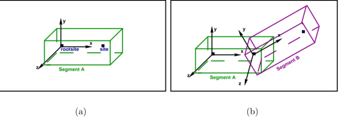
Each segment has at least two sites and one of them is rootsite of the seg-ment (see Figure 2.1.a). A site is an attachseg-ment point on a segseg-ment. A joint connects the site of a segment to the site of another segment (see Figure 2.1.b). The location of the axes of the joints defines the placement of the segments. This provides flexibility on the length and the shape of the segments. All transformations are provided by the joints.
site rootsite y x z Segment A (a) y x z Segment A Segment B z y x (b)
Figure 2.1: (a) segment representation; (b) two segments connected with a joint.
Each joint can have six DOFs (three for rotational and three for trans-lational). The number of DOFs of an articulated structure is the number of independent position variables necessary to specify the state of a structure [33]. Articulated figures have only rotational DOFs. A rotation with a correspond-ing angle around the axis of the DOF forms a transformation and the product of transformation matrices of the DOFs belonging to the same joint defines the location of the site and the segment. A DOF includes the rotation axis, current joint angle and the upper and lower limits of the joint angle (see Figure 2.7).
In order to use this segment and joint representation in the construction of an articulated figure, it is convenient to use a tree-structured hierarchy. A site is selected as root site of this hierarchical structure. Normally, the joints represent the edges and the segments represent the nodes in the tree struc-ture (see Figure 2.3). Each joint has a local coordinate frame that describes the transformation of the segment with respect to its parent segment and has a global coordinate frame that describes the transformation of the segment with respect to the root segment. This hierarchical structure provides that the transformation at the parent node affects the displacements of child nodes.
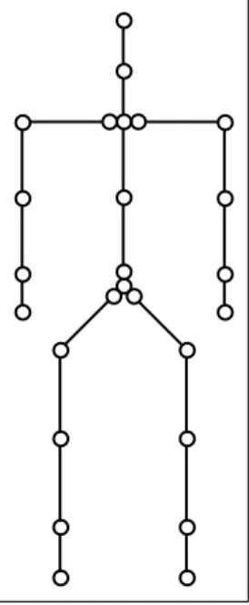
Figure 2.2: Placement of joints on the articulated figure.
In Figure 2.2, joints are represented with circles. Circles at the end of the limbs are end-effectors.
Each branch of the tree is defined as a joint group. Joint group provides a way to handle relevant joints as a whole. A joint group consists of not only joints but also a linear constraint matrix (see Figure 2.8). Linear constraint matrix is constructed by the upper and lower limits of the joint angles. Its use will be explained in detail in Chapter 5.
2.2
Data Structures
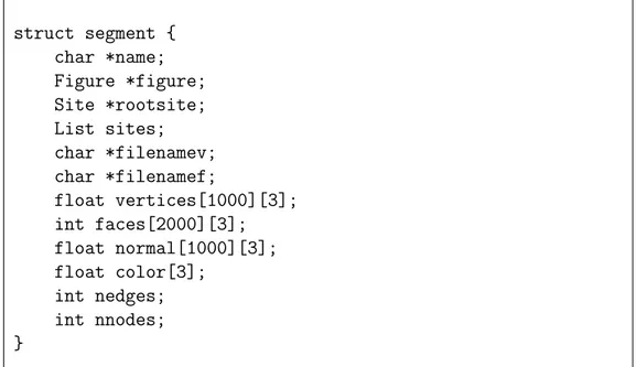
Each segment has an unique name (see Figure 2.4). The rootsite field is helpful to determine the displacement of segment. All sites belonging to a segment are stored in a linked list. The color of the segment is defined in color field. Since the other fields are related with the geometric model of a body (figure), they will be explained in Section 2.3.
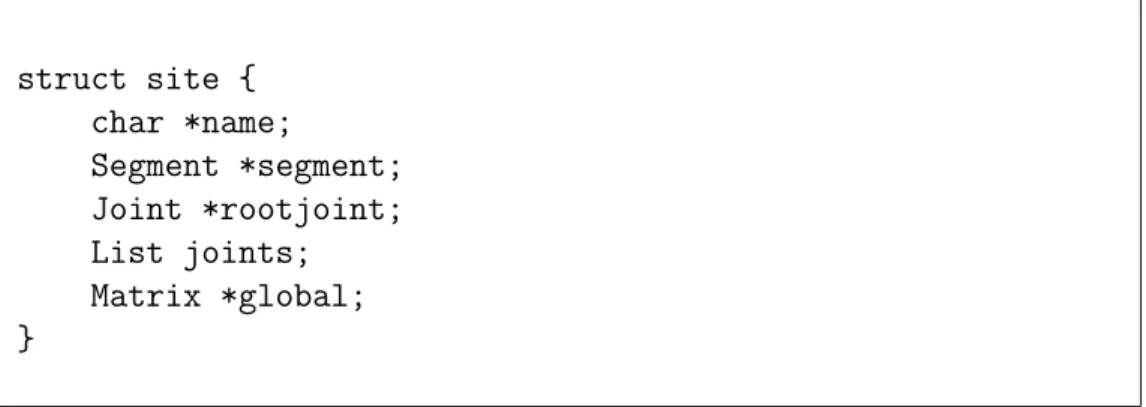
The site is defined with name. The segment field indicates the segment to which the site belongs. The rootjoint field gives the joint that connects the site to the site of neighbor segment. If this site is the root site of the segment
right pelvis left clavicle left left left right clavicle right right right right right right left left left rootsite left pelvis l_pelvis r_pelvis l_hip l_knee r_knee l_ankle l_clavicle r_clavicle r_shoulder r_elbow r_wrist l_shoulder l_elbow l_wrist r_hip neck sacrum waist neck skullbase thigh calf foot low torso up torso skull upperarm forearm hand upperarm forearm hand thigh calf foot r_ankle
Figure 2.3: Tree-structured hierarchy of human figure.
struct segment { char *name; Figure *figure; Site *rootsite; List sites; char *filenamev; char *filenamef; float vertices[1000][3]; int faces[2000][3]; float normal[1000][3]; float color[3]; int nedges; int nnodes; }
struct site { char *name; Segment *segment; Joint *rootjoint; List joints; Matrix *global; }
Figure 2.5: Site data structure
then the neighbor segment is the parent segment of the segment to which the site belongs. The site can be connected to more than one joint. These joints are stored in a linked list. global field stores the transformation of the site with respect to the root segment (see Figure 2.5).
Since all computations are done using the fields of the joints, the joint has a key role in the data structure. The site1 and site2 fields indicate the sites which are connected by the joint. The rootjoint field indicates the parent of the joint in tree-structured hierarchy. Joint’s DOFs are stored as a linked list in the dofs field and the ndofs field stores the number of the DOFs of the joint. The displacement field is a vector that gives the translation of the joint with respect to the parent joint. global is a transformation matrix that gives the position and orientation of the joint with respect to the root segment. The joint group it belongs field defines the joint group of the joint. Index of the joint in the joint group is stored in the index of joint in JointGroup field (see Figure 2.6).
The type field in dof structure defines that it is either rotational (‘r’) or translational (‘t’). Since the joints in articulated figures have no translational DOF, this field currently has no usage. The axis of the DOF is set once and it never changes. The angle changes if a motion occurs on DOF. The llimit and ulimit fields give the lower and upper limits of DOF respectively. The pointer to the next DOF of the same joint is stored in next field (see Figure 2.7).
struct joint {
char *name;
Site *site1, *site2; Joint *rootjoint; DOF *dofs; int ndofs; Vector displacement; Matrix global; JointGroup *joint_group_it_belongs; int index_of_joint_in_JointGroup; }
Figure 2.6: Joint data structure
struct dof { char type; float axis[3]; float angle;
float llimit, ulimit; dof *next;
}
struct group_member { Joint *joint; } struct joint_group { int group_number; int number_of_dofs; float group_angles[20]; int number_of_linear_constraints; float linear_constraints_matrix[25][25]; int number_of_members; GroupMember member[20]; }
Figure 2.8: Joint group data structure
members in the group are stored. Group angles are obtained from DOF angles of the joints in the group (see Figure 2.8).
2.3
Geometric Body Modelling
In order to animate a human figure, the geometry of the body must be mod-elled. This encapsulates constructing a surface or a volume geometry for the human body shape.
2.3.1
Geometric Body Modelling Techniques
In this subsection, current geometric modelling schemes are briefly reviewed. Geometric models can be classified into three categories:
Stick models: Segments are defined as lines. Joints link these segments. Figure
Surface models: Surface models can be grouped as polygons and curved
sur-faces.
The polygonal models are defined as networks of polygons forming 3D polyhedra. Each polygon consists of some connected vertex, edge, and face structure [2].
Mathematical formulations are used for constructing true curved sur-faces called patches. There are many formulations of curved sursur-faces, including: Bezier, Hermite, bi-cubic, B-spline, Beta-spline, and rational polynomial [5, 11].
Volume models: Volume models can be grouped as Voxel models and CSG.
In Voxel models, space is completely filled by a tessellation of cubes called voxels (volume elements). In CSG, there is no requirement to tessellate the entire space. Also, the primitive objects are not limited to cubes. There are many number of simple primitives such as cube, sphere, cylinder, cone, half-space, etc. Each primitive is transformed or deformed and positioned in space.
2.3.2
Surface Scheme with Triangular Polygons
In our application, a polygonal representation is used to model the geometry.
Each segment has a physical shape constructed by triangular polygons. Two files are read for each segment (see Figure 2.4). One of the files consists of point coordinates with respect to the rootsite local coordinate frame (see ure 2.9). These coordinates are written to a 2D array, vertices (see Fig-ure 2.4). The other file stores the polygon (face) information where triangles are used as polygons (see Figure 2.10). These connections are written to an-other 2D array, faces (see Figure 2.4). The normals of the faces are stored in normal field of the segment structure.
The resulting shape for the vertex and face lists presented in Figures 2.9 and 2.10 can be seen in Figure 2.11.
v 0.0 0.0 0.0 v 1.0 0.0 0.0 v 0.0 1.0 0.0 v 0.0 0.0 1.0
Figure 2.9: An example file showing the 3D coordinates of points.
f 0 1 2 f 1 2 3 f 0 1 3 f 0 2 3
Figure 2.10: An example file that stores the polygon (face) information.
x
z
y
(0,0,0) (1,0,0) (0,1,0) (0,0,1) point 0 point 1 point 2 point 3Human Animation Techniques
In this chapter, we give an overview of the previous work that has been pro-duced in this area.
In computer graphics, a variety of human animation techniques have been produced. These techniques can be classified into three main categories:
• kinematics, • dynamics, and • motion capture.
3.1
Kinematic Methods
Kinematics studies the geometric properties of the motion of the objects inde-pendent from the underlying forces that cause the motion.
3.1.1
Forward Kinematics
Forward kinematics explicitly defines the state vector of an articulated figure at a specific time. The state vector is
Θ = (θ1, ..., θn), (3.1)
where Θ is the set of joint angles including independent parameters defining the positions and orientations of all joints belonging to the figure.
A set of joints linked to each other hierarchically, forms a chain (i.e. a branch of tree at Figure 2.3). The most distal end of this chain is called the end-effector. With a given Θ, the cascaded transformations of joints in the chain affect the displacement of end-effector (Equation 3.2).
X = f (Θ). (3.2)
This specification is done with the manual input of a small set of poses (key-framing) by animator explicitly. In order to generate intermediate poses (in-betweens), interpolation techniques are used.
The choice of an adequate interpolation technique is a problem. The in-terpolated values for a single DOF between two key-frames form a trajectory curve. Most of the studies are concentrated on to form a proper shape for this trajectory and to control the variations of the speed along the trajectory in or-der to obtain a realistic motion [4, 20, 22, 30]. Linear interpolation technique, piecewise splines and double-interpolant methods with some modifications have been used to generate the intermediate poses.
Forcing the user to specify values for parameters is often inconvenient, es-pecially for tasks with too many DOFs. Too many parameters to control, drive the animator to make errors. In addition to this, combined effects of trans-formations from root to end-effector make it difficult to control the positional constraints while creating a key-frame. During interpolation, obtaining the true trajectory for realistic motion is also hard job to achieve.
Forward kinematics is successful for animating simple objects, but it is not really a good choice for animating highly articulated figures.
3.1.2
Inverse Kinematics
In inverse kinematics, the desired position and orientation of the end-effector are given by the user. Inverse kinematics computes all joint angles in the chain that orient the end-effector to the desired posture. In order to derive Θ with a given X, the inverse of Equation 3.2 is required (Equation 3.3).
Θ = f−1(X) (3.3)
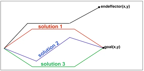
Solving the Equation 3.3 is quite difficult. Since the function in Equation 3.3 is nonlinear, there may be more than one solution set of Θ for a given X (Figure 3.1). In one approach, as the nonlinear property of function makes
goal(x,y) endeffector(x,y)
solution 1
solution 2
solution 3
Figure 3.1: Given goal, more than one solution.
the solution difficult, the problem can be made linear by localizing around the current operating position [34]. Girard’s PODA animation system is an example using this approach [15].
Another numeric approach is nonlinear optimization technique. This ap-proach tries to minimize a function of relation between the end-effector’s po-sition and the user defined goal. It applies iterative non-linear optimization techniques to obtain the minimum. Jack1 animation system developed at the
University of Pennsylvania uses this approach [1, 38].
Tolani et al. [32] also offer a combination of analytic and numerical methods 1Jack is a registered trademark of Transom Inc.
to solve inverse kinematics problems. These approaches will be discussed at Chapter 4 in detail.
3.2
Dynamic Methods
In kinematic approaches, articulated figures are animated with geometric com-putations. However, laws of physics have an important effect on the motion of articulated figure in reality. In computer animation, simulating the physical behavior of objects can produce more realistic motions.
The fundamental principle of dynamics is Newton’s law which can be for-mulated as;
F = ma, (3.4)
where F represents the force applied to an object, m represents mass of the object and a represents its acceleration, which is the second derivative with respect to time of the position vector. The force is linked to the resulting motion (Equation 3.4). The same equation can also be formulated as follows:
T = i¨θ, (3.5)
where T represents the torque, i represents the inertia matrix, and ¨θ represents
the angular acceleration. Torque is linked to rotation (Equation 3.5).
3.2.1
Forward Dynamics
Forward dynamics applies Equations 3.4 and 3.5 in order to calculate the mo-tion with a given force. Equamo-tions 3.4 and 3.5 are only for a rigid body. A hierarchy of rigid parts linked by joints is constructed in order to apply them to an articulated figure.
Animator applies external forces to rigid bodies. The motion is calculated step by step in time. At each step, acceleration is computed with respect to the applied forces. Computed acceleration is twice integrated to the position of the rigid body. The fundamentals of forward dynamics can be found in [35].
It is harder to solve the equation for an articulated structure than for a single rigid body. There is one equation for each DOF and the obtained accel-eration from the equation affects the forces applied to adjacent segments. High computation cost of forward dynamic approaches prevents them to be used in real time applications.
3.2.2
Inverse Dynamics
Inverse dynamics applies Equations 3.4 and 3.5 in order to calculate the forces with a given motion. Some of the notable research using inverse dynamics can be found in [3, 6, 18, 36].
Witkin, Fleischer, and Barr [36] uses “energy” constraints to assemble 3D models, for changing the shape of parametrically-defined primitive objects. Constraints are expressed as energy functions, and the energy gradient followed through the model’s parameter space. The constraints are satisfied if and only if the energy function is zero.
Isaacs and Cohen [18] does physical simulation of rigid bodies, for the spe-cial case of linked systems without closed kinematic loops. They embedded the key-frame animation system within a dynamic analysis by the help of kinematic constraints. Joint limit constraints are also handled through kinematic con-straints. This provides to escape to define additional forces. Instead, kinematic constraints remove constrained DOFs of joints, and inverse dynamic handles unconstrained DOFs.
Barzel and Barr [6] build objects by specifying geometric constraints. They classified these constraints as point-to-nail that fixes a point on a body to a user-specified location in space, point-to-point that forms a joint between two bodies, etc. Each rigid body is independently simulated at each time step. A rigid body is subjected to external forces and constraint forces. These forces act until all the constraints are satisfied. Constraint forces are solved from a set of dynamic differential equations.
spacetime constraints. The main idea is to compute the figure motion and the
time varying muscular forces on the whole animation sequence instead of doing it sequentially in time. The discrete values of forces, velocities and position over time are put in a large vector of unknowns. A set of constraints between these unknowns is specified. The vector of unknowns is computed with a constrained optimization. A cost function is specified for minimization. This function consists of the sum of squared muscular forces over time.
As it has been emphasized in forward dynamics, approaches based on dy-namic simulation suffer from high computational cost compared with the kine-matic approaches. However, the motion of the figure in dynamic approaches is more realistic than that in kinematic approaches.
3.3
Motion Capture
Since each individual has his own motion style, kinematics and dynamics stay insufficient to detect this competence. Moreover, for many different motions, it cannot be possible to obtain them realistically. In recent years, progress in motion capture techniques make it possible to use human motion data directly.
Magnetic and optical technologies make it possible to obtain and to store positions and orientations of points on the human body. However, the stored data are raw and need to be processed. Mostly, the synthetic skeleton does not match with the real one. In [7, 24], the synthetic skeleton is adapted to another one by recovering angular trajectories. They used an inverse kinematic optimization algorithm to obtain the correct angular trajectories. It is also possible to have some errors during capturing because of calibration error, electronic noise etc. These techniques also take care of this problem.
In recent years, two new techniques have been introduced in order to arrange interaction between synthetic actors: motion blending and motion warping. Motion blending technique constructs a database of characteristic motions and produces new motions by interpolating between parameters of this defined motions. Motion warping obtains well-known trajectories and changes the
motion by modifying these trajectories.
Animation techniques based on motion data produce realistic motions. However, this realism depends on the modifications done by the animator and capturing the correct motion data.
Inverse Kinematics
This chapter discusses the solution methods for the inverse kinematics ap-proach. These methods are classified into three categories:
• analytical methods, • numerical methods, and
• a combination of analytic and numerical methods.
Analytical methods can only be used for very simple articulations, like a two-link arm. For more complex articulations, no analytical solutions exist.
4.1
Numerical Methods
4.1.1
Linearized solutions
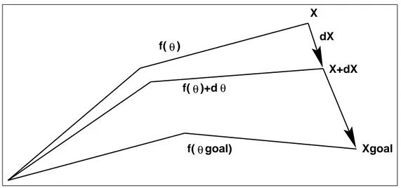
Inverse kinematics problem is nonlinear since the joint transformations involve rotations. This method tries to solve the nonlinear inverse kinematics problem with linear solution. As a first step, Equation 3.2 is differentiated with respect to Θ,
dX = J(Θ)dΘ, (4.1)
f(θ) f(θ)+d f(θ θ goal) X dX X+dX Xgoal
Figure 4.1: Iteration steps towards the desired goal.
where X is the end-effector position and orientation and Θ is the vector of joint angles from the root of the hierarchy to the end-effector and Jacobian J is a matrix of partial derivatives relating differential changes of Θ to differential changes in X
J = ∂f
∂θ. (4.2)
If we invert Equation 4.1 and iterate towards a final goal position with incre-mental steps, inverse kinematics problem can be solved linearly (Figure 4.1).
dΘ = J−1(dX). (4.3) Usually, it is not possible to take the inverse of Jacobian matrix. Because in order to invert Jacobian matrix, it is supposed to be square and nonsingular. However, it is commonly rectangular, because the dimension of Θ is usually larger than that of X. In this situation, pseudoinversion techniques are brought into play [15, 19]. Instead of J−1, pseudoinverse of Jacobian written as J+, is
used and it is defined as follows:
J+= JT(JJT)−1. (4.4) Then, Equation 4.3 becomes,
dΘ = J+(dX). (4.5)
Pseudoinverse solutions have the following problem. The rectangular structure of the Jacobian causes redundancy. A manipulator is considered kinematically
redundant when it possesses more DOFs than needed to specify a goal (Fig-ure 3.1). It is often useful to consider exploiting the redundancy in an attempt to satisfy some secondary condition. This can be accomplished by adding a new term to Equation 4.5,
dΘ = J+(dX) + (I − J+J)dZ, (4.6) where I is the identity matrix, (I − J+J) is a projection operator on the null
space of the linear transformation J, and is called the homogeneous part of the solution. dZ describes a secondary task in the joint variation space. Whatever the secondary task is, the second term does not affect the achievement of the main task. In addition to prevent the redundancy, the secondary task is used to account for joint angular limits [15] and to avoid kinematic singularities [27].
Another problem is the singularity of the Jacobian. Even though the pseu-doinverse can be used when the Jacobian is singular, as the articulation moves, there may be sudden discontinuities in the elements of the computed pseu-doinverse due to the changes in the rank of the Jacobian. Physically, the singularities usually occur when the articulation is fully extended or when the axes of separate links align themselves [33].
With singular value decomposition (SVD), it is possible to analyze whether Jacobian matrix is singular. The details of SVD approach can be found in [25]. Generally, the approaches to prevent the singularity track this situation and when it occurs, they try to avoid from singularity. However, the analysis of the Jacobian for singularity condition brings extra processing cost.
4.1.2
Nonlinear Optimization
Optimization based methods approach the problem as a minimization problem. Let e(θ) be the positional and orientational definition of end-effector depending on joint angles and g be the positional and orientational definition of desired goal,
P (e(θ)) = (g − e(θ))2, (4.7) where P (e(θ)) is a potential function that gives the distance (positional and orientational) between the end-effector and the goal. If the value of potential
function is zero, then the goal is reached. If the goal is not reachable because of the joint limits, the potential function value is tried to be minimized sufficiently. The optimization problem can be formulated as follows [14]:
Minimize P (e(θ)),
subject to li ≤ θ ≤ ui for i = 1, . . . , n. (4.8)
Here, li and ui are the lower and upper limits of the joint angles, respectively.
There are solvers, for example in MATLAB package [31], in order to handle constraint-based nonlinear optimization problems. They can be used as a black box and be integrated to an animation package. However, it is obvious that this integration would increase the computation cost drastically. Therefore, we choose to embed an optimization algorithm into our implementation. The details of the nonlinear optimization method will be explained in the next chapters.
4.2
A Combination of Analytic and Numerical
Methods
Tolani et al. [32] offer a combination of analytic and numerical methods to solve generalized inverse kinematics problems including position, orientation and aiming constraints. They develop a set of algorithms for arm or leg.
They approach the problem with transformation and rotation matrices. A seven DOF limb is defined that has 3 joints. Each of first and last joints has three DOF and joint at the middle has one DOF rotating around y axis. Let us call the joints as J1, J2 and J3, respectively. The equation that has to be
solved in order to reach the defined goal for the limb is
T1ATyBT2 = G, (4.9)
where T1 and T2 denote the rotation matrices of J1 and J3 as functions of three
DOFs belonging to the related joint. Ty is the rotation matrix of J2 defined as
matrices from J1 to J2 and J2 to J3, respectively. Finally, G is the matrix of
the desired goal.
In order to solve Equation 4.9 analytically, trigonometric equations are gen-erated from it. These analytic equations are enough for positional goals, and positional and orientational goals. However, for aiming goals, and positional and partial orientational goals, a combination of analytic and numeric meth-ods is used. Seven variables are reduced to two variables with trigonometric equations, The details of this method can be found in [21]. An unconstrained optimization algorithm is applied to solve for these two variables.
Analytical methods offer high performance for arm or leg limb in computer animation but may require special kinematic structure for the entire body be-cause of the huge trigonometric computations needed. Tolani et al. [32] offers an approach in which an inverse kinematics problem is broken into subprob-lems [39] that can be solved with the analytical method.
Implementation Details
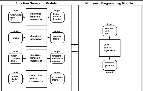
The animation system consists of two main parts:
• the Function Generator Module, and • the Nonlinear Programming Module.
Figure 5.1 gives an overall structure of the animation sytem.
5.1
Function Generator Module
First of all, the human figure is placed to an initial configuration according to the joint parameters entered by the user. The following parameters are entered by the user for each joint to specify the initial configuration of the human figure:
• the angle θ that rotates around an arbitrary vector (x, y, z), • displacement vector with respect to the parent joint, and • the parent joint of the joint.
type, Chain, goal Θ Jacobian Matrix Chain, initial Θ Chain, Potential function calculator Jacobian generator Gradient function calculator value of function Scalar Jacobian Matrix Gradient an array function as Matrix Constraint Gradient, etc. Θ, λ, Line search algorithm Gradient, potential, γ input input input input output output output output input output
Function Generator Module Nonlinear Programming Module
Constraint matrix constructor Chain
Figure 5.1: The overall structure of the animation system.
A transformation matrix M is constructed for each joint,
MJi = TJi(tx, ty, tz)RJi(θ, rotation axis), (5.1)
where TJi(tx, ty, tz) is four by four translation matrix with respect to the parent
joint, RJi(θ, rotation axis) is four by four rotational matrix that gives the
rotation around the axis of the DOF. If we concatenate the individual rotation and translation matrices, then the matrix MJi will be a four by four matrix
that has the following form:
MJi= 0 RJi 0 0 tx ty tz 1 . (5.2)
If the joint has more than one DOF then the general transformation matrix for the joint is obtained by cascaded multiplication of the rotation matrices for each of the principal axes (Equation 5.3), and then by concatenation of the translation and rotation matrices (Equation 5.4).
MJi = TJi(tx, ty, tz)RJi. (5.4)
The implementation of the system can be explained through a simple example. Consider a three-joint articulated structure. Joint parameters of the initial configuration is given in (Figure 5.2). If we write Equation 5.1 for joint J2 in our example, then we obtain
TJ2 = 1 0 0 0 0 1 0 0 0 0 1 0 0 5 0 1 , and RJ2= 0.707 0.707 0 0 −0.707 0.707 0 0 0 0 1 0 0 0 0 1 , MJ2 = TJ2(0, 5, 0).RzJ2(45, z axis), MJ2 = 0.707 0.707 0 0 −0.707 0.707 0 0 0 0 1 0 0 5 0 1 .
MJi only gives the transformation of ith joint with respect to (i−1)th joint.
In order to calculate transformation of jth joint with respect to ith joint, we should do cascaded multiplications:
MJij = MJi.MJi+1...MJj−1.MJj. (5.5)
If the ith joint is the root joint, then MJij gives the global position and
orien-tation of jth joint with respect to the root. If we apply Equation 5.5 to our example then we obtain
MJ12 = MJ1.MJ2, MJ13 = MJ1.MJ2.MJ3, MJ1= 0 1 0 0 −1 0 0 0 0 0 1 0 0 0 0 1 , MJ2 = 0.707 0.707 0 0 −0.707 0.707 0 0 0 0 1 0 0 5 0 1 , and
Joint 1(root) { name: J1 rootjoint: J1 displacement: {0,0,0} number of dofs: 1 axis of dof: {0,0,1} angle of dof: 90 degree } Joint 2 { name: J2 rootjoint: J1 displacement: {0,5,0} number of dofs: 1 axis of dof: {0,0,1} angle of dof: 45 degree } Joint 3 (end-effector) { name: J3 rootjoint: J2 displacement: {-4,4,0} number of dofs: 1 axis of dof: {0,0,1} angle of dof: 0 degree }
Figure 5.2: Joint parameter values for the initial configuration of a three-joint articulated structure.
MJ3 = 1 0 0 0 0 1 0 0 0 0 1 0 −4 4 0 1 . MJ12 = −0.707 0.707 0 0 −0.707 −0.707 0 0 0 0 1 0 0 5 0 1 , and MJ13 = −0.707 0.707 0 0 −0.707 −0.707 0 0 0 0 1 0 −4 9 0 1 .
These cascaded matrix multiplications give the global position and orienta-tion of related joint with respect to the root joint. After the initial configuraorienta-tion of the figure, new DOF axes of each joint are determined and set from obtained global matrix of the joint. These DOF axes are never changed again. When a motion is detected, only angles are changed and new position and orientation of each joint is constructed. In our example, if the joint J3 has one DOF around x axis then, the axis of the DOF will be set to (−0.707, 0.707, 0). During a motion, any angle set for the DOF will rotate around (−0.707, 0.707, 0).
5.1.1
Potential Function Calculation
Potential function P (e(θ)) is a function of the difference between the end-effector and the goal positions and orientations. It should be a nonnegative real number. The motivation behind the nonlinear optimization is to decrease this difference by trying to obtain a value for the potential function as close to zero as possible. In order to measure this difference, first of all we have to define the end-effector. Defined as the most distal joint in the chain, the end-effector can be thought as a 9D vector on the distal segment. First three components define the position of it as a positional vector. Second and third triples are the unit vectors specifying the orientation. The angle between these two unit vectors should be 90 degrees so that they can specify the orientation.
It is obvious that the end-effector is a function (e(θ)) of the state vector that is defined as in Equation 3.1. An instance of the joint angles θ of all the
joints in the chain determines e(θ).
For each joint in the chain, we have a rotation matrix for rotation an-gle θ around the joint axis, and cascaded multiplication of rotation matrices, corresponding to as many as the number of DOFs of the joint, construct a transformation matrix with respect to the parent joint. Cascaded multiplica-tion of these transformamultiplica-tion matrices from the root joint to the related joint gives the transformation matrix of related joint with respect to the root joint. Multiplication of the global matrix, which is constructed at initial position, with the transformation matrix gives the new position and orientation of the related joint. If this related joint is end-effector, we can obtain position vector and the two unit vectors of the end-effector from all these matrix multipli-cations. For example, the joint angles belonging to the chain of joints from sacrum to the left wrist changes the position and orientation of joints in the chain. Finally, the position and orientation of the left hand e(θ) are obtained.
Since the goal is definite constant and the end-effector position and orien-tation change with the joint angles, we can write the potential function as a function of the end-effector P (e(θ)). Usually, all components of the end-effector are not used in order to compute the potential function because of different types of goal.
In order to calculate the potential function P (e(θ)), we have to define the goal types. Although more types of goal are defined in [38], we defined two types of goal in our implementation because of time restrictions:
• positional goals, and
• positional and orientational goals.
A positional goal is defined as a 3D point vector in space. Therefore, only the positional vector of end-effector is used in order to compute potential function for a positional goal. If we define the positional goal as rg and the
position vector of end-effector as re then the potential function becomes,
Since the value of potential function is supposed to be a nonnegative scalar value, it is computed as the square of the difference.
Even though it is possible to define the orientational goal separately, we implemented the combination of positional and orientational goals. In addition to the coordinates of the goal rg in space, orientation of the goal is defined by
two orthonormal vectors xg and yg. Two orthonormal unit vectors of
end-effector xe and ye are used together with positional vector re. The potential
function becomes
P (re, xe, ye) = wp(rg− re)2 + wo((xg− xe)2+ (yg− ye)2). (5.7)
where wp and wo are weights of position and orientation, respectively. The
priorities of position and orientation are adjusted by the weights and the sum of wp and wo is equal to one.
The problem with equation 5.7 is that the values generated by the orienta-tion part are too small according to the values generated by the posiorienta-tion part. In order to reach to one unit difference at position part, one radian difference is needed at orientation part. To arrange this, the term corresponding to the orientation part is multiplied with a scalar value k = 360/(2πd), compensates one length unit to d degrees. Then, for positional and orientational goals, potential function becomes
P (re, xe, ye) = wp(rg − re)2+ wok2 ³ (xg− xe)2+ (yg − ye)2 ´ . (5.8)
5.1.2
Jacobian Generation
Chosen constraint based nonlinear optimization algorithm needs the derivatives of e(θ) with respect to the joint angles, Θ = (θ1, θ2, . . . , θn),
∂e ∂θ = Ã ∂e ∂θ1 ∂e ∂θ2 . . . ∂e ∂θn ! . (5.9) ∂e
∂θ is called the Jacobian matrix. As we know from the Section 5.1.1, re is
the point vector of end-effector, xe and ye are the unit vectors of end-effector
e(θ). And they are computed with cascaded multiplications of four by four
θi in the chain be unit vector u. Then, the derivatives of e(θ) with respect to θi become ∂re ∂θi = u × (re− ri), (5.10) ∂xe ∂θi = u × xe, (5.11) ∂ye ∂θi = u × ye. (5.12)
Each of Equations 5.10, 5.11, and 5.12 is a vector equation. For a joint group with n joint angles, the dimension of the Jacobian matrix is 9 × n.
5.1.3
Gradient Function Calculation
The gradient of the potential function is necessary for the nonlinear optimiza-tion algorithm implemented. Gradient of the potential funcoptimiza-tion P (re, xe, ye) is
a 9 × 1 column vector formed by partial derivatives of the potential function with respect to the re, xe and ye:
∇e(θ) = ∂P ∂re ∂P ∂xe ∂P ∂ye = ∇rP (re) ∇xP (xe) ∇yP (ye) . (5.13)
Each of partial derivatives ∂P/∂re, ∂P/∂xe, ∂P/∂ye is a 3 × 1 column vector.
For positional goals, the values of ∂/∂xe and ∂/∂ye are set to zero.
For positional goals, gradient of Equation 5.6 is
∇rP (re) = 2(re− rg). (5.14)
For positional and orientational goals, gradient of Equation 5.6 is formed by the following equations:
∇rP (re) = 2(re− rg), (5.15)
∇xP (xe) = 2k2(xe− xg), (5.16)
5.1.4
Constraint Matrix Construction
Let us equalize P (e(θ)) to a function of joint angles
G(θ) = P (e(θ)). (5.18)
As it is explained before if we decrease the value of G(θ) to zero then we reach the goal. However, it is not always possible because of the joint angle limits. For this reason, G(θ) is minimized:
Minimize G(θ),
subject to li ≤ θi ≤ ui for i = 1, . . . , n. (5.19)
Here li and uiare lower and upper joint limits, respectively. In order to use the
joint limits in our nonlinear optimization algorithm, they have to be rearranged as linear equality and inequality constraints:
aT
i θ = bi for i = 1, 2, . . . , l (5.20)
aTi θ ≤ bi for i = l + 1, l + 2, . . . , k
where ais are n×1 column vectors and the total number of them is k. The total
number of θs is n. l of ais represent equality constraints. Inequality constraint
representation is in the form of −θi ≤ −li, and θi ≤ ui.
In order to clarify, let us support formation of constraints with an example:
θ1 = π, π/4 ≤ θ2 ≤ π/2 ⇒ −θ2 ≤ −π/4, θ2 ≤ π/2, −π/4 ≤ θ3 ≤ π/4 ⇒ −θ3 ≤ π/4, θ3 ≤ π/4, Then ATΘ ≤ B, 1 0 0 0 −1 0 0 1 0 0 0 −1 0 0 1 × θ1 θ2 θ3 ≤ π −π/4 π/2 π/4 π/4 .
5.2
Nonlinear Programming Module
There are two major families of algorithms for multidimensional nonlinear mini-mization with calculation of first derivatives. Both families require a line search sub-algorithm. The first family goes under the name conjugate gradient meth-ods. The second family goes under the names quasi-Newton or variable metric methods. Since both of the methods are for unconstrained nonlinear equations and there is no superiority to each other, we used to a modification of variable metric method which is more common than conjugate gradient method.
Variable metric methods come in two main flavors. One is the Davidon-Fletcher-Powell (DFP) algorithm. The other goes by the name Broyden-Fletcher-Goldfarb-Shanno (BFGS). The BFGS and DFP are used together in our implementation.
Algorithm can be briefly defined in five steps:
1. Guess an initial feasible Θ.
2. Form an approximation to Hessian matrix H updated with constraints. 3. Compute a search direction d = −Hg(θ).
4. Find θ = θold+ λd using a line search to insure sufficient decrease.
5. Check the result whether the function is at the minimum (Kuhn-Tucker point), then stop else go to step 2.
g(θ) at step 3 is the gradient of objective function G(θ), g(θ) = ∇θG ⇒ g(θ) = Ã ∂e ∂θ !T ∇eP (e(θ)), (5.21)
where the Jacobian matrix ∂e/∂θ is computed by the Jacobian Generator Mod-ule and ∇eP (e(θ)) is computed by the Gradient Function Calculator Module.
In fact, the computation of g(θ) belongs to the Gradient Function Calculator Module. At each iteration, the Nonlinear Programming Module requests the objective function and its gradient from the Function Generator Module.
At each iteration, the value of objective function G(θ) decreases monoton-ically, and stops at a minimum value.
The Nonlinear Optimization
Algorithm
6.1
Determining an Initial Feasible Point
In nonlinear optimization, the key to stability and rapid convergence is an ini-tial guess of joint angle set not too far from the final result. Iniini-tially, we assign zero to each joint angle and select the goal next to end-effector. However, the important condition is that zero value will satisfy the equality and inequality constraints, else the value near zero is selected. If the selected goal is too far away from end-effector, we divide the goal into subgoals and run the algorithm more than once for in-between goals until reaching the desired goal. The joint angles found for an in-between goal become the initial feasible joint angle set for the next in-between goal. If the motion is changed to another direction by the user, the zero values are assigned to the joint angle set again and the optimization process continues. An initially selected joint angle is feasible if it satisfies equality and inequality constraints.
Another property of the algorithm is that the user interacts with initial joint angles by assigning a scalar multiplier to them, meanwhile the implementation takes care of joint limits. Nonlinear algorithm gives higher priority to the variables that have greater partial derivatives. When the multiplier scales the
joint angle, it also scales the derivative as well. The user can arrange the priority of joint angles with this method. This provides the user to escape creating unrealistic motions.
6.2
Active Constraints
If a constraint is an equality constraint or in an inequality constraint, given θi
satisfies the equality in border, then this constraint is active. For example, at an inequality constraint θi ≤ ui, if with a given θi, θi = ui equality is satisfied then
constraint becomes active. Nonlinear optimization algorithm that we choose handles the active constraint. This situation affects our constraint matrix and needs a modification on constraint matrix. Let us examine the example given in Subsection 5.1.4: θ1 = π (constraint 1), −θ2 ≤ −π/4 (constraint 2), θ2 ≤ π/2 (constraint 3), −θ3 ≤ π/4 (constraint 4), and θ3 ≤ π/4 (constraint 5).
Let initial Θ vector be specified as θ1 = π, θ2 = π/3, and θ3 = −π/4. Then,
1 0 0 0 −1 0 0 1 0 0 0 −1 0 0 1 × π π/3 −π/4 ≤ π −π/4 π/2 π/4 π/4 .
Constraint 1 is an active constraint, because it is an equality constraint. Constraint 4 is an active constraint because it is at the border. Then, we have one active equality constraint, one active inequality constraint and three inac-tive inequality constraints. In order to bring the constraint matrix convenient
for operations in the algorithm, we have to swap and shift the rows of matrix in a way that first q (i.e. 2) rows of k (i.e. 5) row matrix will be active constraints:
1 0 0 0 0 −1 0 −1 0 0 1 0 0 0 1 × π π/3 −π/4 ≤ π π/4 −π/4 π/2 π/4 .
6.3
Linearly Constrained Nonlinear
Optimiza-tion Algorithm
Variable Metric Method has been introduced by Davidon [9] for the uncon-strained problem as described by Fletcher and Powell [13] (hereafter called the DFP algorithm). The DFP algorithm has been improved and the BFGS algorithm has been introduced [8, 12, 17, 28]. In his original paper, Davidon envisaged the extension of his algorithm for unconstrained minimization to the case of linear equality constraints. Goldfarb [16] extended the DFP algorithm to the problem of linear inequality constraints by utilizing the techniques de-scribed by Rosen [26] in association with his projected-gradient method by which the search direction determined from the corresponding unconstrained problem is orthogonally projected to the subspace defined by those constraints on variables. At each iteration, a number of the constraints are regarded as being active and on that set of constraints, an equality problem is solved. The algorithm we presented here is taken from [38]. It is a combination of the BFGS algorithm and Rosen’s projected-gradient method.
An iterative algorithm calculates the least value of objective function G(θ) of n variables subject to equality and inequality constraints as in Equation 5.19. Because the algorithm is iterative, it requires an initial estimate of the solution
θ0 and then for i = 0, 1, 2, . . . the ith iteration replaces θi by θi+1, which should
be a better estimate of the solution. All the calculated angles θi are forced
to satisfy the constraints. The termination condition of algorithm is Kuhn-Tucker point. For detailed explanation about the Kuhn-Kuhn-Tucker point, readers
are referred to [14]. The steps of algorithm are presented as follows [38]:
1. θ0 is an initial feasible n size joint angle set, and H0
0 is an initially chosen
n-by-n positive definite symmetric matrix which is identity matrix in our
application. A is n-by-m constraint matrix where m denotes the sum of all active and inactive constraints and q of them are active at point θ0.
Aq is composed of q column vector ai of A, and the first l columns of Aq
are equality constraints ai : i = 1, 2, . . . , l. Hq0 is computed by applying
Equation 6.3 q times; g0 = g(θ0). 2. Given θi, gi, and Hi q, compute Hqigi and α = (AT qAq)−1ATqgi If HT
q gi = 0 and αj ≤ 0, j = l + l, l + 2, . . . , q, then stop. θi is a
Kuhn-Tucker point.
3. If the algorithm did not terminate at Step 2, either
kHi
qgik > max{0, 1/2αqa−1/2qq } or kHqigik ≤ 1/2αqa−1/2qq , where it is
as-sumed that αqa1/2qq ≥ αia−1/2ii , i = l + 1, . . . , q − 1, and aii is the ith
diagonal element of (AT
qAq)−1. They are all positive [16]. If the first
inequality holds, go to Step 4, Else drop the qth constraint from Aq, and
obtain Hi q−1 , from Hi q−1 = Hqi+ Pq−1aiqaTiqPq−1 aT iqPq−1aiq (6.1)
where Pq− 1 = IAq−1(ATq−1Aq−1)−1ATq−1 is a projection matrix; aiq is the
qth column of Aq; and Aq−1 is the n-by-(q1) matrix obtained by taking
off the qth column from Aq.
Assign q − 1 to q,and go to Step 2.
4. Compute the search direction di = −Hi
qgi for line search sub-algorithm,
and compute λj = bj− aTjθi aT jdi , j = q + 1, q + 2, . . . , k λi = min{λ j > 0}
We used and modified the routine lnsrch from [25] for line search to obtain the biggest possible γi such that 0 < γi ≤ min{1, λi}, and
P (θi+ γdi) ≤ P (θi) + δ 1γi(gi)Tdi g(θi+ γdi)Tdi ≤ δ 2(gi)Tdi (6.2)
where δ1 and δ2 are positive numbers such that 0 < δ1 < δ2 < 1 and
δ1 < 0.5. Let θi+1 = θi + γidi and gi+1 = g(θi+1). If (gi)Tdi > 0 which
means the function value would not be decreased, then recompute the search direction as di = −gi and run the step 4 again.
5. If γi = λi, add to A
q the aj corresponding to min{λj} in Step 4 (by
swapping aj with aq+1). Then compute
Hi+1 q+1 = Hqi− Hi qajaTjHqi aT jHqiaj (6.3)
Assign q + 1 to q and i + 1 to i, and go to Step 2.
6. Else, set σi = γidi and yi = gi+1− gi, and update Hi
q as follows:
If (σi)Tyi ≥ (yi)THi
qyi then use the BFGS formula:
Hqi+1= Hqi+ µµ 1 + (yi)THqiyi (σi)Tyi ¶ σi(σi)T − σi(yi)THi q− Hqiyi(σi)T ¶ (σi)Tyi (6.4)
Else use the DFP formula:
Hqi+1= Hqi+ σ i(σi)T (σi)Tyi − Hi qyi(yi)THqi (yi)THi qyi (6.5)
Assign i + 1 to i, and go to Step 2.
6.4
Discussion
We obtained the best result with δ1 = 0.0001 and δ2 = 0.5. In the
optimiza-tion algorithm, choosing the initial values that decrease the funcoptimiza-tion value sufficiently, is crucial. Else the algorithm can be failure. Especially, while we are changing the direction of a limb to an opposite site, initial values obtained from the previous computation may cause the algorithm to be failure. In ad-dition, since there are usually more than one solution, initial guess affects the
generated solution. This situation takes control away from the user. As it is explained in Section 6.1, we tried to obtain solution that is desired by the user, by multiplying the initial values with scalars.
The algorithm searches for a local minimum along a direction d in line search sub-algorithm. Sometimes, (gi)Tdi > 0 is occurred which means that it
cannot find local minimum. Therefore, we modified the algorithm as in step 4 and we changed the search direction.
Results
Our human figure consists of 20 segments, 26 joints and 31 DOFs. Four of the joints were defined as the end effectors. These are right and left hands, and right and left feet. Four joint groups were defined. The left upper joint group includes the joints from pelvis to left hand with 9 DOFs. The right upper joint group includes the joints from pelvis to right hand with 9 DOFs. The left lower joint group includes the joints from pelvis to left foot with 8 DOFs. The right lower joint group includes the joints from pelvis to right foot with 8 DOFs.
The left and right joint groups have three common DOFs on torso. If any motion is applied to one of these joint groups, an unrealistic appearance at the segments of the other joint group may occur, since the segments are separated (see Figure 7.1.a). However, tree-structured hierarchy of the human figure enables us to pass the motion on to the other joint group since any change at the position of the parent segment effects all of the child segments (see Fig-ure 7.1.b).
The algorithm only works for one goal instead of multiple goals at each time. Figure 7.2.a is an example of a reachable goal and Figure 7.2.b shows an unreachable goal.
As it is explained in Section 6.1, a scalar multiplier can be assigned to the joint angles. In Figure 7.3.a, an undesirable posture comes out without assigning a scalar multiplier. While the joint angles rotating around the x axis
(a) (b)
Figure 7.1: (a) unrealistic posture; (b) realistic posture.
is sufficient to reach the goal, the joint angles rotating around y and z axes, have initial values that effect the direction of the line search. In order to reach the defined goal in Figure 7.3.b, the joint angles, except the angles rotating around the x axis, are multiplied with 0.1. The priority of the joint angles rotating around the x axis is increased with this way. The algorithm handles them first.
(a) (b)
Figure 7.2: (a) reachable goal; (b) unreachable goal.
7.1
Performance Experiments
Totally, 899 vertices have been used to draw the segments. Average fps results during motion have been presented at Table 7.1 for the situations that are lights on/off and wireframe/mesh. The results were obtained on a personal computer with Intel Pentium1 III – 550 Mhz CPU and 192 MB of main memory with 32
MB of graphics memory.
Table 7.1: Average frame rates for animations
Wireframe/Mesh Shading Average FPS
Wireframe Shaded 13.90
Wireframe Not shaded 26.65
Mesh Shaded 14.05
Mesh Not shaded 29.05