Investigation of the effects of MAS5, RMA and GCRMA preprocessing methods on an affymetrix zebrafish genechip dataset using statistical and network parameters

(1)

i

INVESTIGATION OF THE EFFECTS OF MAS5, RMA AND

GCRMA PREPROCESSING METHODS ON AN AFFYMETRIX

ZEBRAFISH GENECHIP

®

DATASET USING STATISTICAL AND

NETWORK PARAMETERS

A THESIS SUBMITTED TO THE DEPARTMENT OF MOLECULAR

BIOLOGY AND GENETICS AND THE INSTITUTE OF

ENGINEERING AND SCIENCE OF BILKENT UNIVERSITY

IN PARTIAL FULFILLMENT OF THE REQUIREMENTS FOR THE

DEGREE OF MASTER OF SCIENCE

By

AHMET RAŞİT ÖZTÜRK

(2)

ii

(3)

iii

I certify that I have read this thesis and that in my opinion it is fully adequate, in scope and in quality, as a thesis for the degree of Master of Science.

________________________________ Asst. Prof. Dr. Özlen Konu

________________________________ Assoc. Prof. Dr. Işık G. Yuluğ

________________________________ Asst. Prof. Dr. Tolga Can

Approved for the Institute of Engineering and Science

_______________________________ Prof. Dr. Mehmet Baray Director of Institute of Engineering and Science

(4)

iv

ABSTRACT

INVESTIGATION OF THE EFFECTS OF MAS5, RMA AND GCRMA PREPROCESSING METHODS ON AN AFFYMETRIX ZEBRAFISH

GENECHIP® DATASET USING STATISTICAL AND NETWORK PARAMETERS

Ahmet Raşit Öztürk

MSc, in Molecular Biology and Genetics Supervisor: Assist. Prof. Özlen Konu

January, 2010, 125 pages

Microarray data preprocessing is an important determinant of the accuracy and repeatability of expression profiling studies. Recent studies have focused on comparison of preprocessing methodologies using differential expression analysis of spike-in datasets and qRT-PCR confirmations. Other approaches include comparison of array-wise and probe-wise correlation and of selected gene network parameters. However, zebrafish GeneChip datasets have not been used in such comparisons; furthermore, detailed analysis of upregulated and downregulated gene sets with respect to known network parameters are not well characterized across different preprocessing methodologies. In this study we re-analyzed a public zebrafish hypoxia microarray dataset (GSE4989; Marques et al. 2008) using MAS5, RMA, and gcRMA methods. Comparisons were made in terms of differentially expressed gene sets and defined network parameters, namely, clustering coefficient, degree distribution, and betwenness centrality. Our findings indicated that gcRMA and RMA exhibited greater similarity to each other in terms of differentially expressed genes, and network parameters. In addition, the network analysis demonstrated that upregulated and downregulated gene sets had distinct network structures; downregulated probesets had greater clustering coefficients and degree distributions for positively correlated probesets in all three preprocessing methods. However, gcRMA and RMA methods accentuated this difference further than MAS5 did, suggesting that preprocessing methods differ in their modulation of gene expression network structure. A selected

(5)

v

group of probesets that showed invariant network structure parameters across RMA, gcRMA and MAS5 was determined and analyzed functionally for the zebrafish hypoxia dataset. The results of this thesis suggest that preprocessing methods may alter network structure of the datasets differentially with respect to upregulated and downregulated gene sets. Accordingly, it might be beneficial to filter differentially expressed genes that are robust to such network topology modulation to increase the repeatability of gene sets.

(6)

vi

ÖZET

MAS5, RMA VE GCRMA ÖN İŞLEME METOTLARININ BİR AFFYMETRIX ZEBRAFISH GENECHIP® VERİ KÜMESİ ÜZERİNE

ETKİLERİNİN İSTATİSTİKSEL PARAMETRELER VE AĞ PARAMETRELERİ KULLANILARAK ARAŞTIRILMASI

Ahmet Raşit Öztürk

Moleküler Biyoloji ve Genetik Yüksek Lisansı Tez Yöneticisi: Yrd. Doç. Dr. Özlen Konu

Ocak, 2010, 125 sayfa

Mikrodizi veri ön işlemesi, ifade profili çıkarma çalışmalarının kesinlik ve tekrar edilebilirliğinin önemli bir belirleyici faktörüdür. Güncel çalışmalar, farklılaşmış ifade analizleri kullanılarak ön işleme metodolojilerinin kontrol probları içeren mikrodizi veri kümeleri ve qRT-PCR doğrulamaları yoluyla karşılaştırılması üzerine yoğunlaşmıştır. Diğer yaklaşımlarsa dizi ve prob boyunca karşılaştırmalarla birlikte, seçilmiş gen ağ parametrelerinin karşılaştırmalarını içermektedir. Ancak zebrabalığı GeneChip veri kümelerinde henüz böyle bir karşılaştırma kullanılmamıştır, ayrıca, bilinen ağ parametreleriyle ilgili olarak anlatımı artan veya azalan gen öbeklerinin detaylı analizi farklı ön işleme metodolojileri üzerinden iyi bir biçimde tanımlanmamıştır. Bu çalışmada bir zebrabalığı hipoksi mikrodizi veri seti (GSE4989; Marques et al. 2008) MAS5, RMA ve gcRMA metodları ile analiz edilmiştir. Karşılaştırmalar, farklı ifade edilen gen öbekleri açısından “öbeklenme katsayısı”, “derece dağılımı” ve “aradalık merkeziyeti” olarak adlandırılan ağ parametreleri referans alınarak yapılmıştır. Bulgularımız gcRMA ve RMA metotlarının farklı ifade edilen genler ve ağ parametreleri açısından daha yüksek bir benzerlik gösterdiğini işaret etmektedir. Bunun yanı sıra ağ analizi, anlatımı artan ve azalan gen öbeklerinin farklı ağ yapılarına sahip olduğunu, pozitif korelasyon gösteren probsetler açısından anlatımı azalan probsetlerin her üç ön işleme metodunda da daha yüksek öbeklenme katsayısı değerleri ve ağ grafiğinde daha fazla bağlantıya sahip olduğunu göstermiştir. Bu durum MAS5 metoduna göre gcRMA ve RMA metotları tarafından işlenen verilerde daha ön plana çıkmıştır. Bu durum da ön işleme metotlarının gen ifade

(7)

vii

ağlarının yapılarını şekillendirmekte farklı etkilerinin olduğunu göstermektedir. RMA, gcRMA ve MAS5 ile ön işlemeye tabi tutulan verilerden oluşturulan ağlar arasında ağ topolojisi bakımından en az değişiklik gösteren bir probset öbeği seçilmiş ve zebrabalığı hipoksi veriseti için fonksiyonel olarak analiz edilmiştir. Bu tezin sonuçları, ağ yapılarının anlatımı artan ve azalan gen kümeleri açısından ön işleme metotları tarafından değiştirildiğini önermektedir. Buna göre, farklı ifade edilen gen kümelerinin tespitinin tekrarlanabilirliğini arttırmak için ağ topolojilerindeki değişimlere dayanıklı genleri filtrelemek yararlı olabilir.

(8)

viii

ACKNOWLEDGEMENTS

I would like to thank to Assist. Prof. Özlen Konu for her supervision, valuable suggestions and for sharing her experiences on bioinformatics during my undergraduate and master studies. It has always been a privilege to work with such a special person.

I would like to express my thanks to Assoc. Prof. Işık G. Yuluğ and Assist. Prof. Tolga Can for their helpful comments for my thesis study.

I am indebted to especially Muammer Üçal, Ceren Sucularlı, Onur Kaya and Rümeysa Bıyık on behalf of all my friends for providing a stimulating environment in the lab. I would like to thank them on their friendship and support.

I would like to attend my thanks to Fatih Semerci for his support for my thesis and my thoughts.

Many thanks to MBG family who were with me during my studies.

(9)

ix

LIST OF FIGURES

Figure 1. Data distribution of each array before preprocessing 15

Figure 2. Raw data expression value frequencies. 16

Figure 3. RMA-preprocessed data expression value

frequencies. 16

Figure 4. gcRMA-preprocessed data expression value

frequencies. 17

Figure 5. MAS5-preprocessed data expression value

frequencies. 17

Figure 6. Comparison of distributions of raw and preprocessed

data. 18

Figure 7. Plots of medians of each raw and preprocessed

datasets. 20

Figure 8. Plots of standard deviations of each raw and

preprocessed datasets. 20

Figure 9. Distribution of intersection of probe sets generated from RMA, gcRMA, and MAS5 preprocessed data. Number of unique probe sets in each category is shown on the figure.

Colored areas are proportional to the number of probe sets. 23

Figure 10. Venn diagram of intersection of probe sets

generated from RMA, gcRMA, and MAS5 preprocessed data. Number of unique probe sets in each category is shown on the

figure. 24

Figure 11. Histogram of correlation values from union data of

each preprocessing method. 26

Figure 12. Histogram of correlation values from intersection

data of each preprocessing method. 26

Figure 13. Distribution of positive correlation values in each

preprocessed union data 27

Figure 14. Distribution of positive correlation values in each

preprocessed intersection data. 27

Figure 15. Sum of edges for networks generated at different

r-value thresholds for union data. 28

Figure 16. Sum of edges for networks generated at different

r-value thresholds for intersection data. 29

Figure 17. Boxplots representing the distribution of

betweenness centrality values in each network for union data. 31

Figure 18. Detailed representation of Figure 17 for better visualization of the distributions between the first and the third

(13)

xiii

Figure 19. Boxplots representing the distribution of

betweenness centrality values in each network for intersection

data. 33

Figure 20. Distributions of clustering coefficients among

different networks, for union data. 35

Figure 21. Distributions of clustering coefficients among

different networks, for intersection data. 35

Figure 22. Degree distribution in different networks, calculated

for union data. 37

Figure 23. Degree distribution in different networks, calculated

for intersection data. 38

Figure 24. Fold change versus clustering coefficient for the networks of intersection data. Red dots represent upregulated

genes. 39

Figure 25. P-value versus clustering coefficient for the networks of intersection data. Red dots represent upregulated

genes. 40

Figure 26. Fold change versus betweenness centrality for the networks of intersection data. Red dots represent upregulated

genes. 41

Figure 27. P-value versus betweenness centrality for the networks of intersection data. Red dots represent upregulated

genes. 41

Figure 28. Fold change versus degree distribution for the networks of intersection data. Red dots represent upregulated

genes. 42

Figure 29. P-value versus degree distribution for the networks

of intersection data. Red dots represent upregulated genes. 43

Figure 30. Scatter plots of clustering coefficients for each

network pair. Red dots represent upregulated genes. 44

Figure 31. Scatter plots of betwenness centrality values for

each network pair. Red dots represent upregulated genes. 44

Figure 32. Scatter plots of degree distribution values for each

network pair. Red dots represent upregulated genes. 45

Figure 33. Fold change versus clustering coefficient for the networks of random data. Red dots represent upregulated

genes. 46

Figure 34. P-value versus clustering coefficient for the networks of random data. Red dots represent upregulated

genes. 46

Figure 35. Fold change versus betweenness centrality for the networks of random data. Red dots represent upregulated

(14)

xiv

Figure 36. P-value versus betweenness centrality for the networks of random data. Red dots represent upregulated

genes. 48

Figure 37. Fold change versus degree distribution for the networks of random data. Red dots represent upregulated

genes. 49

Figure 38. P-value versus degree distribution for the networks

of random data. Red dots represent upregulated genes. 49

Figure 39. Scatter plots of clustering coefficient values for each network pair or random data. Red dots represent upregulated

genes. 50

Figure 40. Scatter plots of betweenness centrality values for each network pair or random data. Red dots represent

upregulated genes. 51

Figure 41. Scatter plots of degree distribution values for each network pair or random data. Red dots represent upregulated

genes. 51

Figure 42. Fold change versus clustering coefficient for both intersection and random networks. Network topology measures

from random data is plotted in yellow. 52

Figure 43. Fold change versus betweenness centrality for both intersection and random networks. Network topology measures

from random data is plotted in yellow. 52

Figure 44. Fold change versus degree distribution for both intersection and random networks. Network topology measures

(15)

xv

LIST OF TABLES

Table 1. Summary of each step of different preprocessing methods (modified from

Lim et al., 2007).. 5

Table 2. Number of differentially expressed genes that are detected by t-test, after

each preprocessing method. 21

Table 3. Numbers of common probe sets among pairs of differentially expressed

gene lists. 22

Table 4. Percentage of common probe sets that are shared in all three differentially

expressed gene lists. 22

Table 5. Numbers of union of differentially expressed gene list pairs. 22

Table 6. Percentage of differentially expressed gene lists to the union of all probe

sets. 22

Table 7. Comparisons of the betweenness centrality distributions of RMA,

gcRMA, and MAS5 preprocessed correlation networks using one-sampled t-test, for

union data. 30

Table 8. Comparisons of the betweenness centrality distributions of RMA,

gcRMA, and MAS5 preprocessed correlation networks using one-sampled t-test, for

intersection data. 31

Table 9. Comparisons of clustering coefficient distributions of RMA, gcRMA, and

MAS5 preprocessed correlation networks using one-sampled t-test, for union data. 34

Table 10. Comparisons of clustering coefficient distributions of RMA, gcRMA, and MAS5 preprocessed correlation networks using one-sampled t-test, for

intersection data. 34

Table 11. Comparisons of degree distributions of RMA, gcRMA, and MAS5

preprocessed correlation networks using one-sampled t-test, for union data. 36

Table 12. Comparisons of degree distributions of RMA, gcRMA, and MAS5

preprocessed correlation networks using one-sampled t-test, for intersection data. 37

Table 13. Spearman correlation rho values of pairwise comparison of each network

topology measure matrix 44

Table 14. Spearman correlation rho values of pairwise comparison of each network

topology measure matrix for random data. 50

Table 15. Least-variant genes in terms of network topology measures for

intersection dataset 55

Table 16. Least-variant genes in terms of network topology measures for union

(16)

xvi

ABBREVIATIONS

DEG : Differentially Expressed Gene

gcRMA : GC Robust Multi-chip Average

GUI : Graphical User Interface

MAS5 : Microarray Suite version 5.0

MM : Mismatch

PM : Perfect Match

qRT-PCR : Quantitative Real Time Polymerase Chain Reaction

(17)

1

CHAPTER 1: INTRODUCTION

1.1. Microarrays in human disease

Every year millions of people die because of various cancer types and other diseases. The reason for most treatment to fail is the lack of understanding of the nature of the disease. Since the cellular mechanisms causing a disease is complex, high-throughput methods are necessary in order to show the relationships between different genes or proteins (Draghici 2003). Bio-molecular interaction networks, which can be partly assessed through characterization of gene expression profiles and can be relatively easily obtained using microarray techniques, provide extensive information to understand the organization and interactivity of a biological system involved in disease (Draghici 2003).

The main advantage of microarrays is the ability of quickly and inexpensively getting the gene expression profile of a certain tissue or cell type at the transcriptome level (Seidel and Niessner 2008). Today, nearly all of the known transcriptome can be mapped and expression values can be obtained (Yauk et al. 2007). This notion gains importance especially in the case of cancer and drug treatment where a certain condition affects the behavior (or in other terms, expression pattern) of a group of cells. Transcriptome studies might be beneficial in the areas of drug development, diagnosis, comparative genomics, and functional genomics (Thorgeirsson et al. 2006; Wiltgen et al. 2007). It’s also important to increase understanding of mechanisms of physiological and cellular processes that might contribute to disease process, such as hypoxia, ischemia, and oxidative stress. Micorarray studies allow for expression profiling at a large scale; and functional annotation of the gene lists obtained from such analyses leads to novel signaling pathway characterizations involved in different pathologies (Quackenbush 2002).

1.2. Zebrafish as a model for human disease and gene networks

Model organisms are widely used in biomedical research (Amatruda et al. 2008; Gonzalez-Nunez et al. 2009). Zebrafish is a model organism that help the researcher find the effect of a condition within a short time due to its high reproductive capacity

(18)

2

and relatively short embryonic and larval development (Dooley et al. 2000). In addition, zebrafish has been shown to share common properties in terms of molecular response in human cancer models such as liver cancer (Berghmans et al. 2005). These characteristics make zebrafish an excellent good organism for studying human disease.

A limited number of protein-protein interaction and gene regulatory networks of zebrafish have been generated in the literature and some web tools generated for the visualization and the basic analysis of those networks also include zebrafish datasets. In a recent study (Sorathiya et al. 2009), a microarray dataset has been normalized using the RMA method and a gene expression network was generated. Network topology analysis revealed a group of genes which may have a role in the early stages of vasculogenesis in zebrafish. In another study (Webb et al. 2009), visualization of an in silico network was performed to identify the effects of amphetamine on gene expression. Other two studies (Bacha et al. 2009; Jupiter et al. 2009) focus on the development of web-based tools for network visualization and analysis using zebrafish protein-protein interaction and gene expression networks for demonstration of the tools.

1.3. DNA microarrays

Several types of microarrays are available for a wide variety of purposes (e.g., DNA, protein, and tissue microarrays). DNA microarrays can be separated into two types as cDNA and oligo arrays where a cDNA or a 25-80 base long oligonucleotide is spotted microscopically onto a solid surface (Schena et al. 1995). Another way of producing microarrays is through lithography where oligonucleotides are synthesized on the array using a special technique of light masking (Pease et al. 1994).

The working principle of microarrays is the hybridization of two oligonucleotides which is detected by the fluorescence emitted during the hybridization process (Draghici 2003). The signal from the oligonucleotide pair is read from special optic devices where the intensity of the signal represents the amount of hybridization for a specific oligonucleotide, namely the amount of gene expression. However, the intensity value can only be interpreted with respect to control spots or intensity values of a set of housekeeping genes (Millenaar et al. 2006; Irizarry, Bolstad, et al. 2003).

(19)

3

Getting a relative gene expression value dictates the necessity of utilizing a normalization method in order to make the comparison between different arrays possible (Geller et al. 2003). Normalization is also necessary to handle the differences between arrays in terms of RNA extraction, labeling, hybridization, and scanning as well as other types of systematic error (Draghici 2003).

1.4. Preprocessing of Microarrays

Although microarray technology promises great advantages, it also has its problems (Quackenbush 2002; Hill et al. 2001; Bilban et al. 2002; Boes et al. 2005; Kreil et al. 2005; Grewal et al. 2007; Canales et al. 2006; Steinhoff et al. 2006; Zakharkin et al. 2005; Smyth et al. 2003). One of the handicaps is the fact that one can obtain relative gene expression values, not the actual ones using the hybridization based techniques (Schena et al. 1995; Geller et al. 2003). Second, since the experimental procedures from RNA isolation to hybridization are error prone and also affected by the experience of the technician, non-biological noise is inserted into the microarray data (Bolstad et al. 2003). In addition, the distribution of different probe sets on different microarray platforms makes the comparison of different studies more difficult (Irizarry, Hobbs, et al. 2003). Although the first problem mentioned depends on the nature of microarrays, the latter ones can be solved through data transformations (Geller et al. 2003). The data preprocessing is a necessary step to remove the non-biological noise from the real signal as much as possible. Several preprocessing and normalization techniques have been proposed including RMA (Irizarry, Hobbs, et al. 2003), gcRMA (Wu et al. 2004), MAS5.0 (Hubbell et al. 2002), dChip (Li et al. 2001), PLIER (Affymetrix), and others (Shedden et al. 2005).

Despite the fact that proposed preprocessing techniques are useful for reducing systematic technical noise, there is no golden standard. One of the suggested methods is MAS5.0, a method proposed and suggested for Affymetrix for data preprocessing. In this method, mismatch probes, with a single mismatch from the perfect match probes, are taken into account for calculating the amount of true hybridization; and a scaling approach is used for data normalization (Hubbell et al. 2002). In addition, many studies use RMA since it has been shown to outperform other preprocessing techniques. RMA depends only on the perfect match probes from the microarray raw

(20)

4

data (Irizarry, Hobbs, et al. 2003; Katz et al. 2006; Bolstad et al. 2003; Chiogna et al. 2009). Another method called gcRMA has been introduced to improve the performance of RMA method by considering the effect of probe GC content (Wu et al. 2004). Although these methods are successfully utilized for the detection of differentially expressed genes (Draghici 2003; Shedden et al. 2005), it is also shown that the array platform, tissue type, sample size of the study, or numerous other conditions can affect the performance of the applied method (Giles et al. 2003).

1.5. Comparative analysis of Preprocessing Methods 1.5.1 Description of Methods

Preprocessing of microarray raw data is a three-step process for Affymetrix data that aims to result in the summed normalized signal intensity measurements (Draghici 2003; Irizarry, Hobbs, et al. 2003). Due to non-specific and false binding, filtering background noise from the data is the first crucial step. This step is called background correction. After filtering out the systematic noise from the data, normalization is applied. Normalization enhances the comparison of different data from different microarray experiments adjusting and scaling the main characteristics of the data, such as mean/median, distribution and/or standard deviation. After the normalization of the signal intensities of each nucleotide, the last step is summarization of the normalized values. Typically, a transcript is represented by 11 to 20 different short oligonucleotides and combining these multiple signal intensities is a crucial operation (Affymetrix). Summarization is usually the last step where signal intensities of multiple oligonucleotides, which represent a single transcript, are collected and summed into a single signal intensity value. Although some methods might have a different order or extra steps during preprocessing (Schuster et al. 2007), preprocessing methods that we refer in this thesis follow the steps mentioned above. A summary of each preprocessing method’s approaches for background correction, normalization, and summarization is shown below (Lim et al. 2007) in Table 1. According to a study in 2009, MAS5 is the most preferred method in the literature for the preprocessing of Affymetrix HG-U133 array whereas RMA is the second preferred method (Kadota et al. 2009).

(21)

5

Table 1. Summary of each step of different preprocessing methods (modified from Lim et al., 2007).

Method Background correction Normalization Summarization

MAS5 MM Subtraction Constant Tukey biweight

RMA RMA transformation Quantile Median polish

gcRMA gcRMA transformation Quantile Median polish

1.5.2 MAS5

As shown in Table 1, MAS5 utilize PM-MM subtraction for background correction. For each oligonucleotide on the array, Affymetrix has designed a corresponding mismatch oligonucleotide in order to take the effect of non-specific binding into account. In addition, the method gives detection calls that represent the presence or absence of the expression of a gene. Using this property of arrays, MAS5 corrects the perfect match signal intensities using mismatch signal intensities for each oligonucleotide. MAS5 assumes a linear approximation of background correction. For the normalization step, this method uses constant scaling to normalize different arrays. Lastly, for summarization, Tukey’s biweight approach is preferred (Hubbell et al. 2002). This summarization method is an efficient method for removing large median absolute deviations from the data. MAS5 removes background noise for each array independent from other arrays in the dataset. Thus, it is a single-chip method for preprocessing. So, preprocessing is not affected by addition or subtraction of arrays to the dataset (Binder et al. 2010).

Robust averages of PM-MM values are calculated in MAS5 method for background correction. However, variation of probes with low signals is increased. Also the subtraction adds extra noise to the data (Pepper et al. 2007). Obtaining MM values larger than PM values is another possible problem of MAS5 method, generally handled by using idealized MM values.

1.5.3. RMA

Due to the ineffective utilization of mismatch probes on the array, a new method was proposed depending just on the perfect match signal intensities (Irizarry, Hobbs, et al.

(22)

6

2003). Another property of this method is the utility of quantile normalization, which is a linear method for array-wise adjustment. Decomposition of the frequency distribution of signal intensities into an exponential signal and a Gaussian background distribution is the main approach of this method. Arrays are then normalized using quantile normalization, which scales the data across arrays in quantiles. Lastly, median polish, a summarization method, is used for getting a single signal intensity value for a transcript from multiple oligonucleotides (Lim et al. 2007). Median polish minimizes the residual log error. As a result, different signal intensities are transformed into one average distribution. RMA method decreases the variance of probes with low signal values (Binder et al. 2010).

1.5.4. gcRMA

gcRMA is the enhanced version of RMA method that uses GC content information of each nucleotide to calculate binding efficiency and thus, signal intensity. Since the strength of G-C hybridization is stronger than A-T, the GC content of an oligonucleotide affects the binding tendency of each oligonucleotide pair after washing the arrays (Wu et al. 2004). Normalization and summarization steps are the same as the RMA method. However, for background correction, gcRMA background correction method is applied (Lim et al. 2007). It is a multi array approach that is affected by addition or subtraction of arrays into a dataset. As a result, weighted averages of arrays are calculated and replaced with the original values (Binder et al. 2010).

1.5.5. Comparative preprocessing method studies and gene networks

In the literature, advantages and disadvantages of each preprocessing method is widely discussed (Kadota et al. 2008; Kadota et al. 2009; Hua et al. 2008; Verhaak et al. 2006; Qiu et al. 2005; Beyene et al. 2007; Liu et al. 2006; Reverter et al. 2005; Fujita et al. 2006; Harr et al. 2006; Shedden et al. 2005; Bolstad et al. 2003; Autio et al. 2009). Although a single method is not superior to others, it is concluded that the efficiency of the method is affected by the nature of the study (Verhaak et al. 2006). In addition, it is stated that MAS5 has more reliable results than other methods when applying a correlation-based statistical analysis like clustering analysis (Lim et al.

(23)

7

2007). In another case, RMA has been found superior when a list of significantly expressed genes was identified (Zakharkin et al. 2005). Although clustering and significantly expressed genes are investigated through different preprocessing methods, comparative gene network analysis has not been widely studied in the literature in this respect, to our knowledge. Most notably, Lim et al. (2007) has introduced the concept of normalization method comparisons in terms of reverse engineering gene networks. Another important landmark was a study performed by Ahn et al. (2009), which compared different networks with each other using specified network characteristics.

Although the generation of the network is usually performed using a correlation method like Pearson correlation (Selga et al. 2009; Baralla et al. 2009), network structure is thought to be robust and main parameters like clustering coefficient is a characteristic property of a network independent of the data (Strogatz 2001; Watts et al. 1998). Since it is shown that different tissue and cell types affect the efficiency of preprocessing method (Shedden et al. 2005; Gyorffy et al. 2009), it should be assessed if different preprocessing methods have significant effects on the network structure and the characteristics of network properties.

1.6. Zebrafish Microarrays

The microarray that is studied in this thesis belongs to the Affymetrix GeneChip Zebrafish Genome Array. The Affymetrix GeneChip Zebrafish Genome Array platform consists of 15,509 different probe sets for the detection of more than 14,900 zebrafish transcripts. Array is designed using the sequences from 2003 builds of RefSeq, Genbank, dbEST, and Unigene sequence databases. Each probeset includes 16 different 25-mer oligonucleotides long probes. Detection sensitivity scale is 1:100,000 (Affymetrix).

According to GEO database, there are currently 46 GeneChip Zebrafish Genome Array series representing 610 samples at the time this thesis is written. To our knowledge, there is no study in the literature focusing on the effects of normalization methods on Genechip Zebrafish Genome Array data. It is shown in the literature that different cell or tissue types can affect the statistical properties of data that affects the performance of preprocessing methods (Gyorffy et al. 2009; Shedden et al. 2005).

(24)

8

CHAPTER 2: AIMS AND STRATEGY

Microarray data analysis includes steps and methods such as preprocessing of raw data, differentially expressed gene identification, clustering, and visualization of gene regulatory networks. In this thesis, the aim is to investigate whether there is an advantage applying either the MAS5, RMA or gcRMA preprocessing algorithms to raw microarray data, using an exemplary dataset from zebrafish, to perform a more accurate gene profiling analysis.

Motivation behind the thesis is that although these three methods have been previously compared using human microarrays from different tissues and experiments, the effect of normalization on Affymetrix Zebrafish arrays has not been studied, to our knowledge. Since preprocessing is likely to affect the analysis results at different levels, better knowledge of the characteristic changes introduced by normalization and development of novel statistical analysis approaches would lead to a) a more suitable selection of normalization methods; and b) a more reliable interpretations of the obtained results.

To achieve the goal of this thesis, zebrafish Affymetrix microarray data on hypoxia

(Marques et al. 2008) were obtained from GEO database of NCBI. The dataset was

normalized using MAS5, RMA and gcRMA. Different analysis approaches were

applied to compare the characteristic effects of the mentioned

normalization/preprocessing methods: 1) assessment of data distribution; 2) assessment of differentially expressed genes; 3) determination and comparison of gene regulatory network characteristics. The reason for using a wide variety of analysis approaches is that different aspects of data characteristics could be influenced by each method. Thus, one can obtain a more thorough understanding of all facets of the problems and/or advantages associated with each method. For example, results of a t-test are affected by the extent of variation for each gene whereas the gene regulatory networks are affected by the relative rank of a gene among samples (Lim et al. 2007).

This thesis also aims to test whether upregulated and downregulated probesets have distinct network structure and properties (i.e., clustering coefficient, degree distribution, and betweenness centrality) in zebrafish hypoxia and normoxia

(25)

9

experiments; and whether these differences are affected differentially by application of microarray preprocessing algorithms. To test this hypothesis, positively correlated edges were used for network comparisons that were made between the up- and down-regulated probesets for each method and between methods using visualization techniques such as scatterplots and correlation analyses, and tests between real and randomized networks.

Finally, we also aimed to identify a subset of significantly differentially expressed probesets, with invariant network properties that are independent of the normalization method using the zebrafish hypoxia dataset. This study will help increase our understanding of the degree to which preprocessing can alter differentially expressed gene lists as well as the network structure in microarray datasets.

(26)

10

CHAPTER 3: MATERIALS AND METHODS

3.1. Dataset

In this study, a public microarray dataset (GSE4989; Marques et al. 2008) was downloaded from the NCBI GEO database (Barrett et al. 2005) to test the effects of normalization on differentially expressed gene lists and gene network characteristics. In GSE4989 expression series, gene expression in response to chronic constant hypoxia in the heart of adult zebrafish has been profiled. Data consisted of 10 Affymetrix GeneChip Zebrafish microarrays, five of which belonged to normoxia and the other five arrays were of the hypoxia group. Maques et al. (2008) identified 376 differentially expressed genes with a p value of 0.05 or less and a minimum fold change of 2. Although not mentioned in the paper, the preprocessing method used by the Marques et al. (2008) was RMA.

Hypoxia is the lack of getting enough oxygen into the body. It can be either generalized or tissue hypoxia depending on the severity and the location of the oxygen deprivation (Semenza 2001). Although mammals are not tolerant to hypoxia, it is known that some teleosts –such as zebrafish- have the ability to cope with extreme oxygen deprivation (Stecyk et al. 2004). The aim of the paper of Marques et al. (2008) has been to identify differentially expressed genes in hypoxia in order to understand the mechanism of developing such a tolerance. They have suggested that understanding the mechanism of zebrafish’s response to chronic constant hypoxia in heart might have clinical implications in the future (Marques et al. 2008). In the present thesis, we aim to test whether such an expression profile is robust to differences in preprocessing methods particularly in terms of differentially expressed gene lists and gene network parameters.

3.2. Preprocessing Methods

MAS5, RMA, and gcRMA methods were utilized to preprocess the raw data obtained in the form of .CEL files. To automate the normalization process, an R script was written using the functions of Bioconductor R packages (APPENDIX A). Once .CEL files were read into a variable, data were preprocessed with the abovementioned

(27)

11

methods and written into a tab separated file for further use (APPENDIX A). In addition, each generated file was also saved in an MS Excel 97-2003 compatible format for further use. Since the rma() and gcrma() methods give log2 transformed data, log2 transformation also was applied to the data obtained from the mas5() function to make the preprocessed data values comparable (BioconductoR).

3.3. Assessment of Differentially Expressed Genes upon preprocessing

Bioinformatics Toolbox of MatLab 2008a was used for the current and the following steps. Once the preprocessed data have been read into variables, samples from each of the two different groups (e.g., hypoxia vs normoxia; GSE4989) were labeled for a t-test (APPENDIX B). matt-test() function was used for calculation of p-values to identify differentially expressed genes by applying this function to each preprocessed dataset; and the probeset lists were obtained. Upon retrieval of the differentially expressed gene lists from each preprocessed data, union or intersection of these lists were obtained using a code that made use of the ‘union’ and ‘intersect’ functions (APPENDIX B).

3.4. Generation and comparison of gene expression networks

To generate gene expression networks, the Pearson correlation values (Equation 1) were calculated for each probe set pair within an experiment (e.g., GSE4989). Covariance of two datasets X and Y is divided by the multiplication of the standard deviations of X and Y.

(Equation 1)

Only the positively correlated gene pairs having an r value greater than or equal to 0.6 were considered to have an edge between them. The positively correlated gene pairs were analyzed in this study to simplify the network generation and decrease complexity. In this approach, each node represented a gene (probe set) and each edge represented coexpression of the two nodes. Resulting graph, a gene expression network, could be shown as an n-by-n matrix, where n is the number of nodes in the graph. A sparse matrix also was generated to be used for further investigation of network topology (APPENDIX C).

(28)

12

The distribution of correlation pairs across different correlation thresholds (Lim et al., 2007) were calculated and plotted using the plotting functions of MatLab. The average value of the positive correlation values from all pairwise probeset correlations (i.e., a mean edge correlation value) was compared between any two preprocessing method. Random networks (Lim et al., 2007) were generated to establish the extent of differences between observed and random correlations for each preprocessed dataset (APPENDIX C).

Since a differentially expressed gene list obtained from each preprocessed data contained different probe sets, the probesets of the union and those of the intersection lists were used to generate networks where all networks had the same number of nodes (APPENDIX D). Frequency distribution plots of bins of correlated pairs were compared among datasets obtained from different preprocessing methods for union and intersection datasets.

In this study, the following network measures were investigated: degree distribution (Newman 2003), clustering coefficient (Watts et al. 1998), and betweenness centrality (Freeman 1977).

Degree distribution is the number of edges in and out of a node.

(Equation 2)

Ci (clustering coefficient of the node i) is the proportion of neighboring subgraphs

having 3 edges and 3 nodes to the number of neighboring subgraphs with 2 edges and 3 nodes (Equation 2; Watts et al. 1998).

(Equation 3)

CB(v) value is the sum of all possible ratios of shortest paths passing the node v over

the total number of those shortest paths (Equation 3; Freeman 1977) where σst(v) is the number of shortest paths from s to t crossing the node v. σst is the total number of shortest paths from s to t.

(29)

13

For these calculations, a set of related functions from the GAIMC BGL Toolbox 4.0 was utilized in Matlab (Anon 2008). This toolbox has been previously used in a brain network analysis study to calculate network properties (Sporns et al. 2007).

Comparison of networks from different preprocessing methods as well as comparison of a network with a randomized counterpart we used a series of methodologies. To find the conserved correlations (i.e., the conserved edges) among the networks of differently preprocessed data, union and intersection methods were used (APPENDIX D). Scatterplots were generated to visualize network parameters in a pairwise fashion between any two preprocessing method. Spearman correlation coefficients for a compared network parameter across probesets (Ahn et al., 2009) were calculated between preprocessing methods for the intersection and union datasets (APPENDIX G).

Paired t-tests were used to test the differences between any two preprocessing method for the three network parameters, separately. Furthermore, data from each preprocessing method was also compared with those from a randomized dataset using paired t-tests (APPENDIX B).

Upregulated and downregulated probeset lists were generated and plotted against the fold change values and p-values obtained, for each preprocesing method separately using plot() function of Matlab (APPENDIX H).

3.5. Zebrafish Gene Symbol Annotation

Affymetrix IDs were converted to corresponding zebrafish gene symbols using Biomart Martview service (Biomart). Affymetrix IDs were given as an input to appropriate fields and associated gene symbols were retrieved using the GUI of the web tool. 8517 genes were found corresponding to the probesets in Affymetrix Zebrafish GeneChip array.

3.6. Drawing Graphs

For the generation of boxplots and histograms, MatLab’s boxplot() and hist() functions were utilized with appropriate input variables (APPENDIX D). In addition, suitable functions of AutoCAD 2008 were used for generating figures 9 and 10.

(30)

14 3.7. Random Network Generation

In order to compare the network topology measures with random networks, the node pairs were randomly shuffled in the upper triangle of the adjacency matrix using the code in APPENDIX E. Accordingly, given a network, the code generates a random network with the same number of nodes and edges. For comparing network results with respect to fold change and p-value distributions, actual networks were compared with random networks sampled from the original normalized dataset keeping the number of probesets the same with the intersection dataset (APPENDIX H)

3.8. Analysis of Hypoxia Dataset

To identify genes that were the least variant in both networks of different preprocessing methods, difference of a network parameter in each network was calculated and converted to its absolute value. Then, sum of the differences were sorted in order to identify the least-changed top 20% of the genes for each network topology measure. Lastly, intersection of the least-changed probeset lists was

(31)

15

CHAPTER 4: RESULTS

4.1. Effects of Preprocessing on Data Disribution

Since each preprocessing method aims to remove non-technical variation in the microarray data in different ways, they alter the distribution of the data differently. In order to show the effects of each preprocessing method, boxplots and histograms were used for visualization of each preprocessed data’s numerical properties. Figure 1 demonstrates that the distribution of the raw data before any kind of preprocessing suggesting that GSE4989 arrays have comparable raw data distributions where 50% of the data resided between log2 values of 6 and 8. Raw data distribution resembled an extreme value distribution (Gumbel 1958) with a small number of probe sets with high expression values whereas close to 50% of the probes accumulated closer to the lower limit of the distribution (Figure 2). Upon preprocessing, raw data distribution has changed drastically; the shape of the distribution was dependent on the type of the preprocessing method (Figures 3, 4, and 5).

(32)

16

Figure 2. Raw data expression value frequencies.

(33)

17

Figure 4. gcRMA-preprocessed data expression value frequencies.

Figure 5. MAS5-preprocessed data expression value frequencies.

Based on the histogram representations, preprocessing procedures altered the data distribution. While RMA and MAS5 have produced distributions closer to normal

(34)

18

distribution, gcRMA led to a distribution with features of bimodality (Figure 3, 4, and 5). To be able to observe each experiment within the experiment set, boxplots were drawn. Figure 6 indicated that each method within itself was highly consistent thus arrays could be compared with each other. However, there were drastic differences with respect to the median values as well as Inter Quartile Ranges (i.e., IQRs, which is described as showing the robust 50% of the data between 25% and 75%) among different methods (Figure 6). Accordingly, MAS5 normalized experiments had higher IQRs when compared to others; the normalization method that generated the least variable experiment set was RMA. gcRMA resulted in a skewed distribution where the lower 95% confidence interval of the boxplots was truncated relative to those obtained using other methods (Figure 6).

Figure 6. Comparison of distributions of raw and preprocessed data.

Different normalizations resulted in different medians (Figure 7). Also seen from the previous boxplot representation of the raw and preprocessed datasets (Figure 6), the mean of the medians from all 10 microarray experiments were less in gcRMA when compared with those from RMA and MAS5 (Figure 7). RMA data followed gcRMA data and had a 1.5 fold greater median value than gcRMA. In RMA, median values of each array seemed to be stable around the expression value of 6.3, in log2. Raw data

(35)

19

exhibited a higher median value compared to RMA, and lower median value compared to MAS5 (Figure 7). Since the raw data was not processed, the figure

reflected the actual median expression values of each probe. In particular, the 8th array

seemed to have an upward shift in expression values which could be observed from the value distribution shown in Figure 6. Since RMA and gcRMA utilizes quantile normalization method normalizing each array via exchange of actual expression

values between arrays, the upwards shift in the 8th array was not observed in data

normalized with RMA or gcRMA. Lastly, MAS5 had the highest median value for each array and also showed the widest data distribution as seen from the Figures 6 and 7. Since MAS5 used a scaling approach for preprocessing of the data, the normalization was likely to be affected by the deviation and shifts in the raw data. The

median of the 8th array of the MAS5 data was shifted upwards as in the raw data.

The differences in the distribution of each preprocessed data also were reflected in the standard deviation of the arrays. As seen in Figure 8, raw data exhibited the least amount of standart deviation among arrays whereas gcRMA had the highest standard deviation values. Raw data was followed by RMA and then MAS5 datasets. One clear observation from Figure 8 was that RMA and gcRMA tended to decrease the variability in distribution across arrays and standardized the distributions of each array in order to make them more comparable.

(36)

20

Figure 7. Plots of medians of each raw and preprocessed datasets.

(37)

21

4.2. Effects of Preprocessing on Differently Expressed Gene Lists

Based on the findings from the histograms and boxplots of data distributions of both the raw and preprocessed data, it was clear that each preprocessing method altered the distribution and original data values in different ways. Therefore, we hypothesized that this situation also might affect the results of statistical tests based on these normalized datasets.

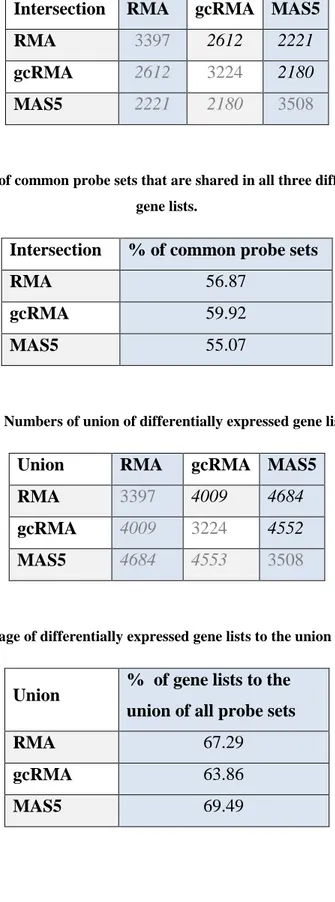
For each dataset, the number of differentially expressed genes was obtained using two sample equal variance t-tests with an alpha value of 0.05; and the results were represented as the number of probesets differentially expressed as well as the corresponding percentage they fell into (Tables 2 and 3). Accordingly, all three methods identified close to 20% of all probesets in the GeneChip as significant. Since gcRMA and RMA were similar in their background correction, normalization and summarization steps, the number of genes common to both methods was greater than that observed between MAS5 and RMA or MAS5 and gcRMA (Table 3). 1932 probe sets were common in these three significant gene lists, each obtained from RMA, gcRMA, and MAS5 preprocessed data, respectively (Table 3). Percentage of the common probesets among these significant gene lists was greater than 50% in all three methods (Table 4). Moreover, the union of these three gene lists consisted of 5048 unique probe sets. Union of significant gene lists of each dataset were compared and results also indicated that RMA and gcRMA gene lists were the most similar ones compared to MAS5 (Table 5). Lastly, Table 6 demonstrated the ratio of significant gene list of each dataset to the union gene list. Accordingly, MAS5 had the biggest contribution to the MAS5 list as expected.

Table 2. Number of differentially expressed genes that are detected by t-test, after each preprocessing method.

# of probe sets % of probe sets

RMA 3397 21.75

gcRMA 3224 20.64

(38)

22

Table 3. Numbers of common probe sets among pairs of differentially expressed gene lists.

Intersection RMA gcRMA MAS5

RMA 3397 2612 2221

gcRMA 2612 3224 2180

MAS5 2221 2180 3508

Table 4. Percentage of common probe sets that are shared in all three differentially expressed gene lists.

Intersection % of common probe sets

RMA 56.87

gcRMA 59.92

MAS5 55.07

Table 5. Numbers of union of differentially expressed gene list pairs.

Union RMA gcRMA MAS5

RMA 3397 4009 4684

gcRMA 4009 3224 4552

MAS5 4684 4553 3508

Table 6. Percentage of differentially expressed gene lists to the union of all probe sets.

Union % of gene lists to the union of all probe sets

RMA 67.29

gcRMA 63.86

MAS5 69.49

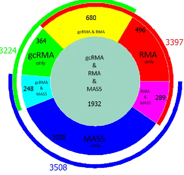
The results were also visualized for a better understanding of the number of probe sets that were commonly or uniquely identified by each one of the methods tested in the present study. Graphical representation and a Venn-diagram representation were

(39)

23

shown in the following figures (Figure 9, 10). Accordingly, each method identified a considerable number of probe sets uniquely, where MAS5 identified the most. Accordingly, gcRMA and RMA were more related to each other in terms of the number of differentially expressed probe sets.

Figure 9. Distribution of intersection of probe sets generated from RMA, gcRMA, and MAS5 preprocessed data. Number of unique probe sets in each category is shown on the figure. Colored

(40)

24

Figure 10. Venn diagram of intersection of probe sets generated from RMA, gcRMA, and MAS5 preprocessed data. Number of unique probe sets in each category is shown on the figure.

4.3. Effects of R-Value Thresholds and Preprocessing Methods on Network Generation

A landmark study performed by Lim et al. (2007) for investigation of the effects of normalization on gene network structure suggested of using a) arraywise correlations of real and randomized datasets; b) distribution of correlation pairs across different correlation thresholds; c) pairwise mutual information between networks; and d) functional enrichment of highly correlated pairs.

In the present study, similarly we tested whether the distribution of correlation pairs across different correlation thresholds differed according to the preprocessing method used. However, instead of analysis of arraywise correlations, we compared the average value of the positive correlation values from all pairwise probeset correlations (i.e., a mean edge correlation value). These comparisons were made between any two

(41)

25

preprocessing method as well as against a randomly generated network as suggested in the Lim et al. (2007) study. In addition, we used paired t-tests instead of mutual information indices to compare the network edge correspondence differences. Finally, frequency distribution plots of bins of correlated pairs were compared among datasets obtained from different preprocessing methods. Our analyses also made use of two different, namely the union and intersection, lists of differentially expressed genes from each method.

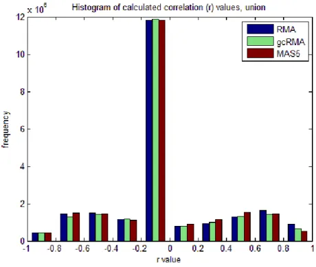
Probeset pairwise correlation value distributions varried from one preprocessing method to another for the union and intersection datasets (Figures 11, 12). For both datasets, correlation values were scattered to the positive and negative ends while most of the correlations were found in between 0 and -0.2. In addition, the intersection dataset had pairwise correlations accumulating at extremes of both directions suggesting a greater proportion of significant pairwise correlations. In the union data, however, except the values between 0.2 and -0.2, correlation values were relatively more uniformly distributed.

Distribution of positive correlation values (r>0) was visualized using boxplot representations (Figures 13, 14). Positive correlation can identify the pairs of genes having a similar expression profile among different arrays. Boxplot representations also showed a similar pattern as observed in Figures 11 and 12. Union data exhibited a more uniform distribution of correlation values whereas the median positive ‘r’ value was higher in the intersection data with lower interquartile of the distribution spanning a greater range of correlation values.

One additional observation from the Figures 13 and 14 was that the effect of preprocessing such that the nature of correlation could be more clearly seen in intersection data. RMA and gcRMA had similar positive correlation profiles whereas MAS5 preprocessed data had relatively lower correlation among pairs of genes. Possible reason for this difference is mentioned in Discussion section.

(42)

26

Figure 11. Histogram of correlation values from union data of each preprocessing method.

(43)

27

Figure 13. Distribution of positive correlation values in each preprocessed union data .

(44)

28

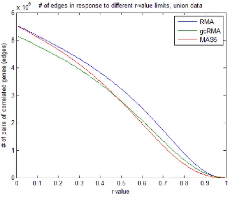
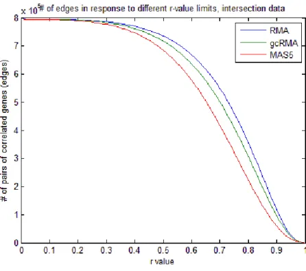
To demonstrate the effects of varying the r-value threshold on the number of edges in each network, distribution of sum of all gene correlations above the threshold (edges) were plotted separately for the union and intersection data (Figures 15, 16). These graphs showed that although there was a slight difference between the correlation distributions of differently preprocessed data, choosing an r-value of 0.6 and greater could minimize the nonlinearity due to methodology. For example, the distribution of all three methods ran parallel to each other when r equaled to or was greater than 0.6. Although RMA- and gcRMA-based correlation values had similar slopes, MAS5-based correlation values decreased faster as the value increased (Figure 15). The r-value around 0.45 was critical in this context so that MAS5-based data became the least correlated in terms of the number of gene pairs. Since intersection data had more significant genes having similar gene expression profiles, MAS5 remained the least correlated data however the slopes were parallel exhibiting linearity among preprocessing methods (Figure 16).

(45)

29

Figure 16. Sum of edges for networks generated at different r-value thresholds for intersection data.

4.4. Effects of preprocessing methods on network structure

To assess the effects of preprocessing methods on network structure, three network topology measures have been widely utilized: betweennes centrality, clustering coefficient, and the degree distribution or connectivity (Barrat et al. 1999; Freeman 1977; Newman 2003). Indeed, these three important network parameters also were previously used in comparison of networks generated from protein-protein interaction, radiation hybrids, functional annotation, and gene expression datasets (Ahn et al. 2009).

4.4.1. Betweenness centrality

Genes located among the shortest paths between any other two genes have a higher betweenness centrality value. Thus, genes with a higher betweenness centrality are thought to have a central role for cellular functions especially having roles for communication between modules (Hintze et al. 2008).

(46)

30

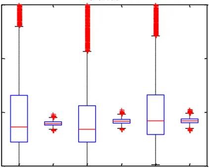
Distribution of betweenness centrality was calculated for correlation networks of each preprocessed data for union (Figures 17-18) and intersection (Figure 19) data. Each preprocessing method was analyzed separately, a boxplot was drawn showing the distribution of the betweenness centrality value distribution when compared with that from a random distribution. Network of original data and random data distribution significantly differed with respect to the range of distribution (Figure 17-19); for both the union and intersection data, RMA, gcRMA, and MAS5 betweenness centrality values were significantly different from their random counterparts with a p-value of zero (less than 10E-16). The random networks were designed to have the same number of genes and pairwise edges, with a randomized correlation distribution. Compared to the random networks, each preprocessed original data had a wide spectrum of betwenness centrality values expected to be seen in a real situation. On the other hand, preprocessing methods did not differ among each other with respect to betweenness centrality data distribution based on the paired-t-tests (Table 7) in the union data. However, usage of intersection data accentuated the differences among the preprocessing methods such that there was an increase in the median and IQR of the between centrality measurements obtained via MAS5 normalization (Table 8). These might show that the different preprocessing methods affected the highly significantly expressed genes in a network setting.

Table 7. Comparisons of the betweenness centrality distributions of RMA, gcRMA, and MAS5 preprocessed correlation networks using one-sampled t-test, for union data.

Betweenness

Centrality gcRMA MAS5

RMA 0.6167 0.0923

(47)

31

Table 8. Comparisons of the betweenness centrality distributions of RMA, gcRMA, and MAS5 preprocessed correlation networks using one-sampled t-test, for intersection data.

Betweenness

Centrality gcRMA MAS5

RMA 0 0

gcRMA 0

RMA RMA-Random gcRMA gcRMA-Random MAS5 MAS5-Random 0 1 2 3 4 5 6 x 105 B e tw e e n n e s C e n tr a lit y Union Data

Figure 17. Boxplots representing the distribution of betweenness centrality values in each network for union data.

(48)

32

RMA RMA-Random gcRMA gcRMA-Random MAS5 MAS5-Random 0 5000 10000 15000 B e tw e e n n e s C e n tr a lit y Union Data

Figure 18. Detailed representation of Figure 17 for better visualization of the distributions between the first and the third quarter.

(49)

33

RMA RMA-Random gcRMA gcRMA-Random MAS5 MAS5-Random 0 200 400 600 800 1000 1200 1400 1600 B e tw e e n n e s C e n tr a lit y Intersection Data

Figure 19. Boxplots representing the distribution of betweenness centrality values in each network for intersection data.

4.4.2. Clustering coefficient

Clustering coefficient is a network topology parameter for measuring the clustering tendency of nodes/genes. Lower clustering coefficients are the indicators of random networks (de Haan et al. 2009). A gene with a higher clustering coefficient is thought to have an actively interacting profile with other genes (Horvath et al. 2008).

To assess the clustering tendency of each network, the clustering coefficient distributions were calculated; boxplotted; and compared with their random networks in pairs (Figures 20-21). Results of comparisons with random networks gave similar results with those of betweenness centrality; clustering coefficients of networks of actual data were significantly different from random counterparts with p-values of zero (less than 10E-16). Strikingly, random networks exhibited very low clustering coefficient values as expected. When the clustering coefficients of RMA, gcRMA, and MAS5 networks were compared in a pairwise fashion, it was observed that clustering coefficient distributions of each preprocessing network was significantly different from each other for both the union and intersection data (Tables 9-10). This

(50)

34

result indicated that the clustering tendency of differentially expressed genes’ were highly affected by the nature of the preprocessing method. Although RMA and gcRMA had very similar protocols for preprocessing, the correction for the GC bias in probesets seemed to have an affect the network structure significantly.

Table 9. Comparisons of clustering coefficient distributions of RMA, gcRMA, and MAS5 preprocessed correlation networks using one-sampled t-test, for union data.

Clustering

coefficient gcRMA MAS5

RMA 0 0

gcRMA 0

Table 10. Comparisons of clustering coefficient distributions of RMA, gcRMA, and MAS5 preprocessed correlation networks using one-sampled t-test, for intersection data.

Clustering

coefficient gcRMA MAS5

RMA 0 0

(51)

35

RMA RMA-Random gcRMA gcRMA-Random MAS5 MAS5-Random 0 0.1 0.2 0.3 0.4 0.5 0.6 0.7 0.8 0.9 1 C lu s te ri n g C o e ff ic ie n t Union Data

Figure 20. Distributions of clustering coefficients among different networks, for union data.

RMA RMA-Random gcRMA gcRMA-Random MAS5 MAS5-Random 0.4 0.5 0.6 0.7 0.8 0.9 1 C lu s te ri n g C o e ff ic ie n t Intersection Data

(52)

36 4.4.3. Degree distribution

Degree distribution or connectivity of a network is another measure for understanding the dynamics of a network. Degree of a node/gene shows the number of its correlated pairs of genes. Connectivity has been shown to be correlated with essentiality of gene function (Caretta-Cartozo et al. 2007).

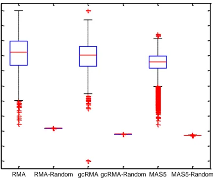
Following figures helped visualize the effects of preprocessing methods on connectivity (Figures 22-23). When compared with the random networks, actual networks were not significantly different (p-values greater than 0.99) in terms of median values for both the union and intersection data. However, when IQR of the actual and random networks were considered, random networks have a much more uniform distribution of node-degree (Figures 22-23). Pairwise comparisons of actual networks were significantly different with very low p-values indicating that the network structure was highly affected in terms of the number of correlations (Tables 10-11). gcRMA and MAS5 resulted in a decrease in nodes with greater number of edges when compared with RMA especially for the intersection dataset (Table 12; Figure 23). Interestingly, random networks also exhibited similar declines in node-degree in the same direction, e.g., RMA>gcRMA>MAS5. Median connectivity was greater in the random network in comparison with the real in RMA and gcRMA, Strikingly, in MAS5 median connectivity of the random network was less than that of the real network.

Table 11. Comparisons of degree distributions of RMA, gcRMA, and MAS5 preprocessed correlation networks using one-sampled t-test, for union data.

Degree

distribution gcRMA MAS5

RMA 0 0