T.C.
SELÇUK ÜNİVERSİTESİ
FEN BİLİMLERİ ENSTİTÜSÜ
TRANSIENT ANALYSIS OF SHORT CIRCUIT FAULTS WITH
REFERENCE TO GRID-CONNECTED WIND/PV HYBRID
SYSTEMS
Farhana Umer
Ph.D. Thesis
Electrical-Electronic Engineering
July 2017
KONYA
iv
TRANSIENT ANALYSIS OF SHORT CIRCUIT FAULTS WITH REFERENCE TO GRID-CONNECTED WIND/PV HYBRID SYSTEMS
Farhana UMER
THE GRADUATE SCHOOL OF NATURAL AND APPLIED SCIENCE OF SELÇUK UNIVERSITY
THE DEGREE OF DOCTOR OF PHILOSPHY IN ELECTRIC-ELECTRONIC ENGINEERING Thesis Advisor: Assist.Prof.Dr. Nurettin ÇETİNKAYA
2017, 154 Pages
Examining Committee Members Prof.Dr. Mehmet ÇUNKAŞ
Assoc.Prof.Dr. Ahmet Afşin KULAKSIZ Assist.Prof.Dr. Nurettin ÇETİNKAYA Assist.Prof.Dr. Hüseyin Oktay ALTUN
Assist.Prof.Dr. Mustafa YAĞCI
Contribution of short circuit current into the transmission network under various fault condition is a significant feature of Wind/PV hybrid power system. It’s a challenging job to protection engineers due to the topology variations among Wind/PV and conventional generating units. This paper presents simulation results for various types of faults and contribution of Wind/PV generators got through transient analysis.
The objective of this research is to examine the transient behavior of a Wind/PV hybrid system due to short circuit faults and resulting waveforms explained the behavior, such as peak values and rate of decay, of the Wind/PV generators. Firstly, a conventional power system is studied, such that the transmission system is fed at one-end by a synchronous generator. Secondly, the power system studied is a hybrid power system in which the conventional power system is integrated with a 100 MW Wind/PV system. Short circuit fault takes place at different locations along a 400 kV transmission line. In this study several scenarios have been considered regarding the types of faults, fault location, fault resistance, Peterson coil and the line lengths. In the studies, ATP/ EMTP program is used for modelling the Wind/PV hybrid power system; As a result, transient overvoltage and overcurrent waveforms are computed and plotted.
Keywords— Transient Analysis; Wind/PV System; Short Circuit Fault; Peterson Coil; Fault Resistance; Overcurrent; Overvoltage and ATP/EMTP
v
vi
First of all, I would like to express my gratitude to God for granting me with wisdom and the opportunity of an education.
My sincere appreciation and gratitude goes to my advisor Dr. Nurettin ÇETİNKAYA for his advice, assistance, encouragement and valuable guidance in the preparation of this work.
I am grateful to acknowledge and thank all of those who assisted me in my doctorate program at Selçuk University. Special thanks are given to my other doctorate committee members Dr. Mehmet ÇUNKAŞ, Dr. Ahmet Afşin KULAKSIZ, Dr. Hüseyin Oktay ALTUN and Dr. Mustafa YAĞCI.
I would like to thank my special friend Engr. Noor KHAN for his support and encouragement throughout this work.
I would like to thank my family members and closest friends, who have been a constant source of inspiration and support throughout my life and academic career.
Acknowledgement is extended to my youngest sister Maryam UMER for her support and cares throughout this work.
vii
TABLE OF CONTENTS
DECLARATION ... iii
ABSTRACT ... iv
ACKNOWLEDGEMENTS ... vi
TABLE OF CONTENTS ... vii
LIST OF FIGURES ... x
LIST OF TABLES ... xv
LIST OF SYMBOLS/ABBREVIATIONS... xvii
1. INTRODUCTION ... 1
1.1 Hybrid Power System ... 1
1.1.1 Transient analysis ... 1
1.2 Research Objective ... 2
1.3 Research Methodology ... 2
2. LITERATURE REVIEW ... 4
2.1 Overview ... 4
3. DISTRIBUTED ENERGY RESOURCES ... 8
3.1 Introduction ... 8
3.2 Photovoltaic System as a Resource of Electric Energy... 8
3.3 Worldwide Growth of Photovoltaics... 8
3.3.1 Estimation for 2015 ... 9
3.4 Photovoltaic Cell ... 9
3.4.1 Voltage-current characteristics and maximum power of PV system ... 10
3.5 Series and Parallel Circuits of PV Cells ... 11
3.5.1 Series connection of solar cells ... 12
3.5.2 Parallel connection of PV cells ... 12
3.5.3 From cells to arrays ... 13
3.6 Classification of PV Systems ... 14
3.7 Wind System as a Resource of Electric Energy ... 14
3.8 Wind Energy System ... 15
3.8.1 Power extracted from wind ... 15
3.8.2 Conversion system for wind energy ... 16
4. COMPUTATIONAL TECHNIQUES OF TRANSIENT ANALYSIS ... 19
4.1 Introduction ... 19
viii
4.1.3 Phase-domain techniques (PDT) ... 21
4.1.4 Graphical techniques ... 22
4.1.5 Root-matching method (RMM) ... 22
4.1.6 State variable method ... 23
5. C OMPUTATION OF SHORT CIRCUT FAULT ... 25
5.1 Introduction ... 25
5.2 Consequences of Faults ... 25
5.3 Fault Statistics for Different Items of Equipment in a Power System ... 26
5.4 Fault Types ... 27
5.4.1 Series faults ... 27
5.4.2 Shunt faults ... 28
6. COMPONENTS MODELLING OF WIND/PV HYBRID SYSTEM IN ATP/EMTP ... 35
6.1 Introduction ... 35
6.2 Synchronous Generator ... 35
6.3 Transmission Line ... 38
6.4 Transformer ... 41
6.4.1 Single phase transformer ... 41
6.4.2 Three phase transformer ... 43
6.5 Induction Generator... 48
6.6 Proposed Mathematical Formulations for the Power System Studied ... 50
7. SIMULATION RESULTS FOR THE PROPOSED WIND/PV HYBRID SYSTEMS ATP/EMTP SOFTWARE ... 53
7.1 Introduction ... 53
7.2 Studied Conventional Power System ... 56
7.2.1 Effect of line length on fault current ... 56
7.2.2 Effect of fault resistance ... 63
7.2.3 Effect of types of fault ... 67
7.3 PV Hybrid Power Systems ... 72
7.3.1 Effect of 3-phase SCF at different location on PV hybrid power system ... 74
7.3.2 Effect of 3-phase SCF on current at PV side i.e. location G ... 76
7.3.3 Effect of fault resistance on PV hybrid system ... 77
7.3.4 Effect of PV system and line length on fault current on PV hybrid system .. 82
ix
7.4.1 Effect of 3-phase SCF at different location on wind hybrid power system ... 87
7.4.2 Effect of 3-phase SCF on current at wind generator side (bus P) ... 90
7.4.3 Effect of fault resistance on wind hybrid system ... 93
7.4.3.1 Effect of fault resistance due to 3-phase SCF ... 101
7.4.4 Effect of wind farm and line length on fault current on wind hybrid system ... 104
7.5 Hybrid Power System Connected with Wind/PV Hybrid System ... 107
7.5.1 Effect of 3-phase SCF at different location on Wind/PV hybrid power system ... 107
7.5.2 Effect of 3-phase SCF current at Wind/PV generator side (bus P and bus G) ... 109
7.5.3 Effect of fault resistance on Wind/PV hybrid system ... 115
7.5.3.1Effect of fault resistance with 3-phase SCF ... 123
7.5.4 Effect of line length on Wind/PV hybrid system ... 126
7.5.5 Comparison between conventional and Wind/PV hybrid power system due to various faults ... 133
7.5.6 Effect of Peterson coil with SCF ... 136
7.5.7 Comparison between Wind/PV GCS with solidly grounding and with Peterson coil under various faults ... 140
8. CONCLUSION AND FUTURE WORK ... 143
8.1 Conclusion ... 143
8.2 Future Work ... 144
REFERENCES ... 145
APPENDIX ... 149
x
LIST OF FIGURES
Figure 3.1 Energy received on the earth’s surface ... 8
Figure 3.2 worldwide growths of photovoltaics ... 9
Figure 3.3 Projected global growth MW ... 9
Figure 3.4 A typical single-crystal silicon PV cell ... 10
Figure 3.5 The equivalent electrical circuit for a solar cell ... 10
Figure 3.6 A typical I -V curve for a solar cell ... 11
Figure 3.7 Maximum power curves for a solar cell ... 11
Figure 3.8 Series Connection ... 12
Figure 3.9 By pass diodes connected across series PV cells ... 12
Figure 3.10 Parallel connections ... 13
Figure 3.11 Forward diodes connected across parallel PV cells ... 13
Figure 3.12 Cells to array ... 13
Figure 3.13 Classification of PV systems ... 14
Figure 3.14 Global net renewable energy generation by fuel type from 2012-2040 ... 15
Figure 3.15 Block diagram of wind system ... 17
Figure 3.16 Constant speed, variable speed and constant & variable speed WECS ... 18
Figure 4.1 Propagation of electromagnetic wave due to fault ... 20
Figure 4.2 Simple RLC circuit ... 23
Figure 5.1 General representation of a LG fault ... 28
Figure 5.2 Sequence network diagram of LG fault ... 29
Figure 5.3 Sequence network diagram of a LL fault ... 30
Figure 5.4 Sequence network diagram of LL fault ... 30
Figure 5.5 General representation of a DLG fault ... 32
Figure 5.6 Sequence network diagram of a DLG fault ... 32
Figure 5.7 General representation of SCF ... 33
Figure 5.8 Sequence network diagram of a SCF ... 33
Figure 6.1 Equivalent circuit of synchronous generator ... 35
Figure 6.2 Line segment ... 38
Figure 6.3 Two port representation of a transmission line ... 40
Figure 6.4 Single phase two winding transformer equivalent circuit ... 41
xi
Figure 6.6 Delta connection of primary side winding ... 45
Figure 6.7 Star-connection of the secondary windings ... 46
Figure 6.8 Block diagram of transformer 1 ... 47
Figure 6.9 Equivalence circuit of Wind/PV hybrid system ... 51
Figure 7.1 Conventional power system (without PV & Wind) studied ... 53
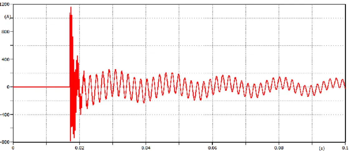
Figure 7.2 Configuration of conventional power system with SLG fault occurs at receiving end ... 56
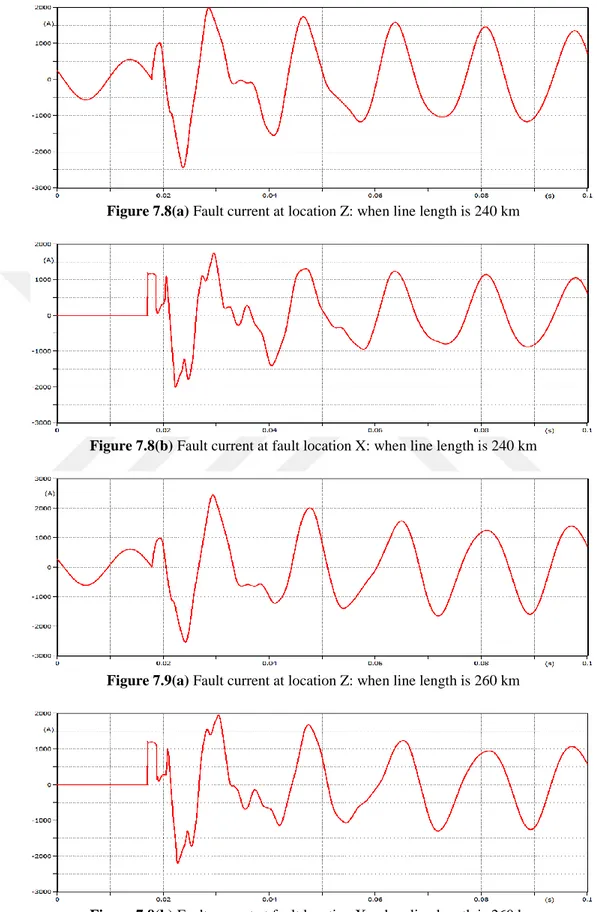
Figure 7.3 to 7.9 Fault current at location Z and X: when line length is 20 km, 100 km, 180 km, 200 km, 220 km, 240 km & 260 km ... 57-60 Figure 7.10 to 7.16 Voltage of un-faulted phases at location Z when line length is 20 km, 100 km, 180 km, 200 km, 220 km, 240 km & 260 km ... 61-63 Figure 7.17 Configuration of conventional power system for fault resistance ... 63
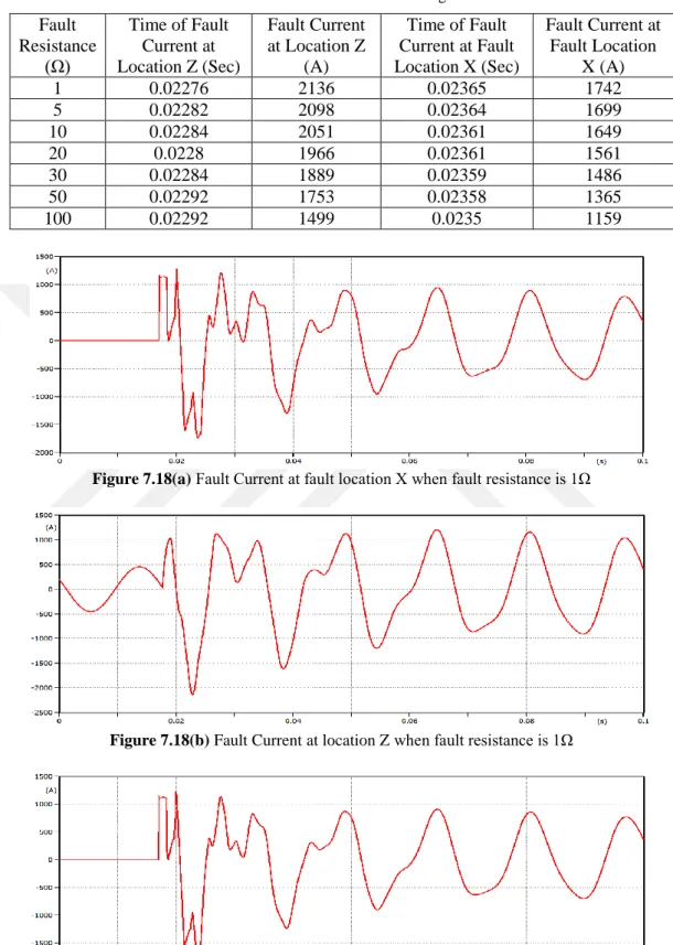
Figure 7.18 to 7.24 Fault Current at fault location X and Z when fault resistance is 1Ω, 5Ω, 10Ω, 20Ω, 30Ω, 50Ω and 100Ω ... 64-67 Figure 7.25 Configuration of conventional power system for 3-phase SCF ... 68
Figure 7.26 Faulted phase current at location Z and X when SLG fault occurs on phase A ... 69
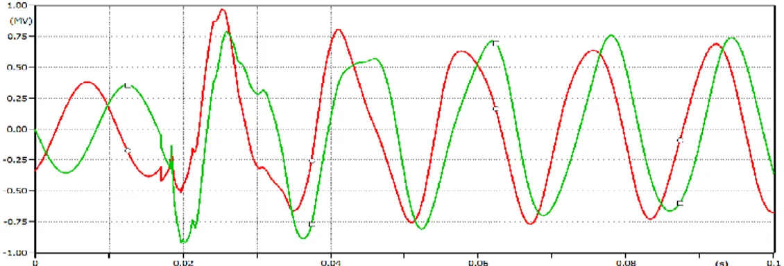
Figure 7.27 Current of faulted phases A and B at fault location X and Z when DLG fault occurs on phases A and B ... 69-70 Figure 7.28 Three phase currents at fault location X and Z when 3-phase SCF occur .. 70
Figure 7.29 Voltages of un-faulted phases at location Z and X when SLG fault occurs on phase A ... 71-71 Figure 7.30 Three phase voltage at location Z and X when DLG fault occur on phases A and B ... 71-72 Figure 7.31 Three phase voltage at fault location X and Z when 3-phase SCF occurs .. 72
Figure 7.32 P-V and V-I characteristic curves of PV ... 73
Figure 7.33 Hybrid power system (with PV only) at no-load ... 74
Figure 7.34 Configuration of PV hybrid system when 3-phase SCF occurs at location A ... 75
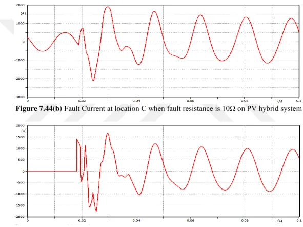
Figure 7.35 to 7.37 Fault current at fault location, when 3-phase SCF occurs at location A, B and C ... 75-76 Figure 7.38 to 7.40 Effect of 3-phase SCF at location G on PV terminal at ac terminal when fault occurs at location A, B and C ... 77
Figure 7.41 Configuration of studied PV hybrid power system: when fault resistance varies from 1Ω to 100Ω with SLG fault occurs on phase A at location A ... 78
Figure 7.42 to 7.48 Fault Current at fault location A and C when fault resistance is 1Ω, 5Ω, 10Ω, 20Ω, 30Ω, 50Ω and 100Ω on PV hybrid system ... 79-82 Figure 7.49 Configuration of studied PV hybrid system: when line length varies from 100 km to 260 km and Effect of line length on fault current ... .83
xii
length is 100 km, 180 km, 200 km, 220 km, 240 km and 260 km ... ...83-86 Figure 7.56 Wind hybrid power system at no-load ... 87 Figure 7.57 Configuration of wind hybrid systems when SCF occurs at bus X ... 88 Figure 7.58 to 7.60 Fault current at fault location, when 3-phase SCF occur at location X, Y and Z on wind hybrid system ... 88-89 Figure 7.61 to 7.63 Effect of 3-phase SCF at bus P on wind generator terminal 34.5 kV side when fault occurs at bus X, Y and Z ... 90 Figure 7.64 to 7.66 Voltages at bus at K: when fault occurs at bus X, Y and Z on wind hybrid system ... 91-92 Figure 7.67 to 7.69 Voltages at bus P: when SCF occurs at bus X, Y and Z on wind hybrid system ... 92-93 Figure 7.70 Configuration of studied Wind hybrid power system: when fault resistance varies from 1Ω to 100Ω with SLG fault occurs on phase A at bus X ... 94 Figure 7.71 to 7.77 Fault Current at fault location X and Z when fault resistance is 1Ω, 5Ω, 10Ω, 20Ω, 30Ω, 50Ω and 100Ω on wind hybrid system ... 94-98 Figure 7.78 to 7.81 3-phase voltages at fault location X and Z: With fault resistance 1 Ω, 10 Ω, 50 Ω and 100 Ω on wind hybrid system ... 99-100 Figure 7.82 Configuration of studied Wind hybrid power system: when fault resistance varies from 1Ω to 100Ω with 3-phase SCF occurs at bus X ... 101 Figure 7.83 to 7.89 3-phase voltages at fault location X: when SCF occurs at fault location X with fault resistance 1 Ω1 Ω, 5 Ω, 10 Ω, 20 Ω, 30 Ω, 50 Ω and 100 Ω on wind hybrid system ... 102-103 Figure 7.90 to 7.94 Fault Current at fault location X on wind hybrid system: when line length is 100 km, 200 km, 220 km, 240 km and 260 km ... ...105-106 Figure 7.95 to 7.98 Voltages of un-faulted phases at location Z on wind hybrid system: when line length is 200 km, 220 km, 240 km and 260 km ... ...106-107 Figure 7.99 Configuration of Wind/PV hybrid system: when 3-phase SCF occur at bus X ... 108 Figure 7.100 to 7.102 Fault current at fault location, when 3-phase SCF occurs at location X, Y and Z on Wind/PV hybrid system ... 108-109 Figure 7.103 to 7.105 Effect of 3-phase SCF at bus P on wind generator terminal 34.5 kV side when fault occurs at bus X, Y and Z ... 110 Figure 7.106 to 7.108 Effect of 3-phase SCF at bus P on wind generator terminal 34.5 kV side when fault occurs at bus X, Y and Z ... 111 Figure 7.109 to 7.111 Voltages at bus at K: when SCF occurs at bus X, Y and Z on Wind/PV hybrid power system ... 112-113 Figure 7.112 to 7.114 Voltages at bus P: when SCF occurs at bas bar X,Y and Z on Wind/PV hybrid power system ... 113-114
xiii
Figure 7.115 to 7.117 Voltages at bus G: when SCF occurs at bas bar X, Y and Z on Wind/PV hybrid system ... 114-115 Figure 7.118 Configuration of studied PV/Wind hybrid power system: when fault resistance varies from 1Ω to 100Ω with SLG fault occurs on phase A at bus X... 116 Figure 7.119 to 7.125 Fault Current at fault location X and Z when fault resistance is 1Ω, 5Ω , 10Ω , 30Ω , 50Ω and 100Ω on Wind/PV hybrid system ... 116-120 Figure 7.126 to 7.129 3-phase voltages at fault location X and Z with fault resistance 1 Ω, 10 Ω, 50 Ω and 50 Ω on Wind/PV hybrid power system ... ...121-122 Figure 7.130 Configuration of studied Wind/PV hybrid power system: with SCF occurs at bus X ... 123 Figure 7.131 to 7.137 SC current at location X: when SCF occurs at fault location X with fault resistance1 Ω, 5Ω, 10 Ω, 30 Ω, 50Ω and 100Ω on Wind/PV hybrid system ... 124-125 Figure 7.138 Configuration of studied Wind/PV hybrid system: when line length varies from 20 km to 260 km ... 126 Figure 7.139 to 7.144 Fault Current at fault location X on Wind/PV hybrid system: when line length is 20 km, 100 km, 200 km, 220 km, 240 km and 260 km ... 127-128 Figure 7.145 to 7.150 Fault Current at location Z on Wind/PV hybrid system: when line length is 20 km, 100 km, 200 km, 220 km, 240 km and 260 km ... 129-130 Figure 7.151to 7.156 Voltages of un-faulted phases at location X and Z on Wind/PV hybrid system: when line length is 20 km, 100 km, 200 km, 220 km, 240 km and 260 km ... 130-133 Figure 7.157 Three phase currents at fault location X when 3-phase SCF occur on conventional system alone and on Wind/PV hybrid system ... 134 Figure 7.158 Faulted phase current at fault location X with SLG fault on conventional system alone and on Wind/PV hybrid system ... 135 Figure 7.159 Current of faulted phases A and B at fault location X when DLG fault occurs on conventional system and on Wind/PV hybrid system ... 135 Figure 7.160 Configuration of studied Wind/PV GCS when Peterson coil varies from 1H to 65H with SCF occurs at bus X... 137 Figure 7.161to 7.165 SC current at fault location X: when SCF occurs at fault location X with fault inductances 1H, 10H, 30H, 58.6 and 65H on Wind/PV GCS ... 137-138 Figure 7.166to 7.170 SC voltage at fault location X: when SCF occurs at fault location X with fault inductances 1H, 10H, 30H, 58.6H and 65H on Wind/PV GCS ... 139-140 Figure 7.171 SCF currents without Peterson coil at fault location X when SCF occur on Wind/PV GCS ... 141 Figure 7.172 SCF currents with Peterson coil of 58.6at fault location X when SCF occur on Wind/PV GCS. ... 141 Figure 7.173 Faulted phase current without Peterson coil at fault location X with SLG fault on Wind/PV GCS. ... 141
xiv
SLG fault on Wind/PV GCS. ... 142 Figure 7.175 Current of faulted phases A and B without Peterson coil at fault location X when DLG fault occurs on Wind/PV GCS . ... 142 Figure 7.176 Current of faulted phases A and B with Peterson coil of 58.6H at fault location X when DLG fault occurs on Wind/PV GC. ... 142
xv
LIST OF TABLES
Table 5.1 Probability of fault occurrence ... 26
Table 5.2 Fault statistics for different equipment in a power system ... 26
Table 5.3 Statistics of faults on overhead TLs at various voltage levels ... 27
Table 5.4 Statistics of faults on overhead TLs at various voltage levels ... 27
Table 7.1 Data of Conventional Generator ... 54
Table 7.2 Data of Hybrid Transformers T1 ... 54
Table 7.3 Data of Transmission Lines TL ... 54
Table 7.4 Serial impedance and shunt admittance of Transmission line 1. ... ..55
Table 7.5 Maximum magnitudes of faulted phase current against line length at sending end Z and faulted location X ... 57
Table 7.6 Effect of Line Length on line Voltage at location Z ... 61
Table 7.7 Effect of Fault Resistance & maximum magnitudes of fault current ... 64
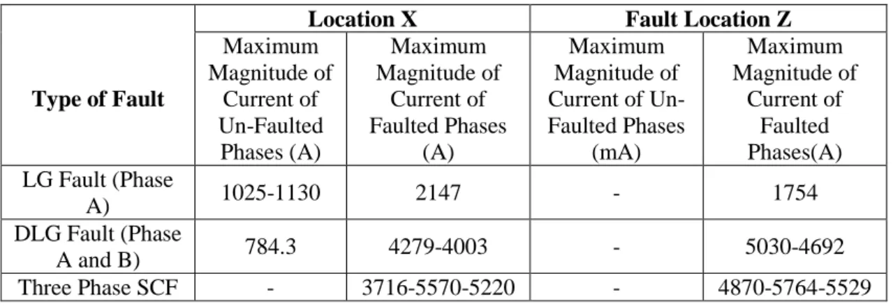
Table 7.8 Maximum magnitudes of fault current at location X and Z for different types of fault on conventional power system ... ....68
Table 7.9 Maximum magnitudes of voltages of faulted and un-faulted phases at locations X and Z for different types of fault on conventional power system ... 71
Table 7.10 Data for PV generator ... 73
Table 7.11 Data of Hybrid Transformers T2 ... 73
Table 7.12 Magnitude of 3-Phase SCF currents at different locations on PV hybrid system ... 75
Table 7.13 Effect of 3-Phase SCF at location G ... 76
Table 7.14 Effect of fault resistance on fault current at location C and fault location A on PV hybrid power system ... 78
Table 7.15 Maximum magnitude of faulted phase current against line length at location C and fault location A and effects of PV on it ... 83
Table 7.16 Data for wind Generator ... 87
Table 7.17 Data of Hybrid Transformers T3 ... 87
Table 7.18 Maximum magnitude of 3-Phase SCF currents when fault occurs at different location on wind hybrid power system ... 88
Table 7.19 Effect of 3-phase SCF at bus P on wind hybrid power system ... 90
Table 7.20 Effect of 3-phase SCF at bus K on conventional generator side and maximum magnitude of Voltages at bus K ... 91
Table 7.21 Effect of 3-Phase SCF on Voltages at bus P ... 92
Table 7.22 Effect of fault resistance on fault current at bus Z and X on wind hybrid power system ... 94
xvi
location X: when SLG fault occurs with fault resistance varies from 1 Ω to 100 Ω ... 98 Table 7.24 Maximum magnitudes of faulted phase currents at fault location X on wind hybrid system due to SLG fault and 3-phase SCF for different fault resistances ... 102 Table 7.25 Maximum magnitude of faulted phase current against line length at location Z and fault location X and effects of wind on it ... 104 Table 7.26 Maximum Magnitude of 3-Phase SCF currents at different locations on Wind/PV hybrid power system ... 108 Table 7.27 Effect of 3-phase SCF at bus P on wind generator side hybrid power system ... 109 Table 7.28 Effect of 3-phase SCF at bus G on PV generator side hybrid power system ... 111 Table 7.29 Effect of 3-phase SCF on at bus K on conventional generator side and maximum magnitude of Voltages at bus K ... 112 Table 7.30 Effect of 3-Phase SCF on Voltages at bus P at wind generator and maximum magnitude of Voltages at bus K ... 113 Table 7.31 Effect of fault resistance on fault current at location Z and fault location X on Wind/PV hybrid power system and its comparison with conventional system alone ... 116 Table 7.32 Maximum magnitude of voltage of un-faulted phases at bus Z and fault location X: with fault resistance varies from 1 Ω to 100 Ω ... 120 Table 7.33 Maximum magnitudes of faulted phase currents at fault location X on Wind/PV hybrid system due to SLG fault and SCF for different fault resistances ... 124 Table 7.34 Maximum magnitude of faulted phase current against line length at location fault location X on Wind/PV hybrid power system ... 127 Table 7.35 Maximum magnitude of faulted phase current against line length at location Z and effects of Wind/PV system on it ... 128 Table 7.36 Maximum magnitude of faulted phase current at fault location X on Wind/PV GCS ... 134 Table 7.37 Minimization of fault currents at fault location X on Wind/PV GCS due to SCF for different values of Peterson coil ... 137 Table 7.38 Comparison between solidly grounding and Peterson coil grounding of 58.6H inductance on Wind/PV GCS under various fault condition ... 141
xvii
LIST OF SYMBOLS/ABBREVIATIONS
SYMBOLS EXPLANATION
ATP Alternative Transients Program
AC Alternating Current
Ra Armature winding resistance
ρair Air density
A Area swept by the rotor blades
β Blade pitch angle
CMRESSS Combined Multiple Renewable Energy Sources System Simulator
Z0 Characteristic impedance of the line
DFIG Double Fed Induction Generator
DLG Double Line-to-Ground Fault
Q Differential operator
Rd D-damper winding resistance
vo Downstream wind velocity
EPIA European Photovoltaic Industry Association EMTP Electromagnetic Transient Program
FF Fill Factor
Flux linkage
IF Fault current
Rf Field winding resistance
f (t) Flux linkage linking field winding
d (t) Flux linkage linking D-damper winding
q (t) Flux linkage linking the Q-damper winding
xviii
F Fault location
GCPS Grid connected photovoltaic system
GUI Graphic User Interface
Zg Ground impedance
GCS Grid Connected Systems
HV High Voltage
XFMR Hybrid Transformer
IGS Integrated Generation System
IG Induction Generator
LG Line-to-Ground
l Length of the line
MPPT Maximum Power Point Tracker
Pmax Maximum power
Km Mass flow rate
NISM Numerical Integrator Substitution Method
PCC Point of Common Coupling
P and O Perturb and Observe
PDT Phase-Domain Techniques
PV Photovoltaic
γ Propagation constant
Rq Q-damper winding resistance
Re Real part of the integration
Rr Radius of turbine blade
RMM Root Matching Method
Rr Radius of turbine blade
xix
SEIG Self-Excited Induction Generator
SPE Solar Power Europe
SG Synchronous Generator
SCIG Squirrel Cage Induction Generator
SCF Short Circuit Fault
VS Sending end voltage
IS Sending end current
TL Transmission Line
PT Theoretical power
TSR Two-Sided Recursions
τ Travel time of the traveling wave
Cg Turn to earth capacitor
nr Turbine rotating speed in rpm
ULM Universal Line Model
WR Wound Rotor
WECS Wind Energy Conversion System
1. INTRODUCTION
1.1 Hybrid Power System
The global reduction fossil-fuel has necessitated an urgent search for alternative energy resources. The wind, PV and hydro sources of energy are inexhaustible, pollution-free, and freely available. The hybrid systems have been considered as attractive and preferred alternative resources (Borowy, 1996; Patel, 2000).
Hybrid power system used number of generation sources i.e. PV, wind, hydro and/or with other conventional systems. PV and wind powers are the most significant part of the globally produced generation (Bhandari and etc., 2015).
1.1.1 Transient Analysis
Transient analysis of faults in hybrid systems is one of the most challenging and vital task. Transients occur in power system due to various reasons resulting because of power system configuration changes i.e. switch opening switch closing, faults, lightning strikes or load variations.
The time of transients is short and equipment faces high transient current and high transient voltage during a transient period. It causes severe damage i.e. thermal stress, fire risk that possibly damages the power system apparatus (Velasco, 2014; Sluis, 2001).
Two types of stress can be caused by transient phenomena in power system
Over-currents
Over-voltages
In order to provide adequate protection against both types of stresses, it’s important to calculate their main features, location and estimate the most unfavourable operating conditions. Accurate analysis of transients is hard due to the size of the system, complexity of the interaction between power devices. Now the study of transients is done with the help of computer (Velasco, 2014).
Power system engineer must understand transients and quantify transients so that, system components are designed to withstand or control transients to avoid damage from high transient voltages and high transient currents. Transients include higher frequencies up to kHz and MHz
When the network changes from one steady state into another transient occurs. It can be due to lightning hits the earth or when it strikes a substation directly. Most of the transient are due to switching action i.e. load disconnect switches. Fuses and circuit breakers interrupt high currents and clear small currents during fault (Sluis, 2001).
Fault contributes the system to an abnormal condition. Transients occur in the system due to various types of faults i.e. SLG LL, DLG and SCFs. SCFs result in a switching action, which often results in transient over-voltages (Velasco, 2014; Sluis, 2001).
1.2. Research Objective
This research examines the behaviour of hybrid power system against transients during symmetrical and asymmetrical faults. The objectives of this research are given below:
Analyse the transients due to symmetrical and asymmetrical faults on a hybrid power system.
Examine the variation of fault currents and voltages under the influence of various factors such as types of faults and fault locations in the hybrid power system studied.
Investigate the transient voltages and currents resulting from various types of faults under the effect of non-linear protective devices.
1.3. Research Methodology
Literature study and collection of data for hybrid power system.
Selection of a hybrid power system (Integration of conventional power system, PV and Wind).
Modelling of PV, Wind and conventional power systems.
Analyse the symmetrical and asymmetrical faults in the hybrid power system considered.
A theoretical background & Literature review is given in Chapter 2. Numerical & theoretical discussion related to distributed generation resources is done in Chapter 3. A theoretical background of different methods of transient analysis for short circuit fault is given in Chapter 4. Types of fault, Mathematical calculation of different types of fault & representation of short circuit faults are given in Chapter 5. In Chapter 6, a representation of transmission system component, generator, hybrid transformer (XFMR) and transmission line models are all presented. A general analysis of the transient short circuit fault is presented in Chapter 7. The analysis presented in Chapter 6 and 7 allow determining the transient short circuit currents and voltages of different system configuration. Chapter 8 summarizes the conclusions of this thesis & few suggestions for future study.
2. Literature Review
2.1 Overview
Several researchers have been studied transient analysis of hybrid power systems due to faults, switching transient etc. Some of such studies are mentioned below.
It has been shown in (Ünver, 1995), that severity of fault and its transient component in transmission systems depends on several factors, such as the magnitude of voltage when fault occur, type of fault and fault location. These factors have important influence on magnitude and shape of voltage and current waveforms.
Demetrios in (Tziouvaras, 2008), use the two-port theory based on symmetrical component transformation for the analysis of simultaneous faults in power systems. Similarly, LEVA applied time-dependent symmetrical components in (Leva, 2009) to study the dynamic analysis of asymmetrical faults in power system. This approach explored Lyon state model of faulted line to examine the transient over-voltages and current due to short circuit.
Wilson and Schmidt in (Wilson, 1974), analysed the behaviour of transmission line for open & short circuit. The voltage and current can be symbolized by both space and partial differential equations, and the solution of such equation become tedious especially when it involves a complex network. But the numerical methods after usage of computers has made the whole process easy and several methods have been developed. Dommel combined the trapezoidal integration for lumped parameters and method of characteristics for transmission lines to solve power system transients (Dommel, 1969). In (Phukan and etc., 2013), a Waveform matching technique is used based on Bare Bones Particle Swarm Optimization techniques of diagnosed short circuit fault.
Valarmathi worked on PV/Wind hybrid system and MATLAB and Model-sim was used for simulation. In this work a VLSI based fuzzy logic controller is used into the hybrid system for supply of continuous power to the grid. Static and dynamic behaviour of the system is analysed. Different type of faults such as LG, LL, DLG and symmetrical faults are studied on 25 kV side of wind generator and also results are
analysed. The results show that hybrid system provided continuous power to the grid under faulty wind farm by means of VLSI based fuzzy logic controller (Valarmathi and etc., 2012).
Jafar Zangina Sulaiman worked on transient behaviour of a hybrid power system (wind and conventional power system) due to SC fault and investigates the effect of type of fault and fault location. EMTP/ATP is used to simulate short circuit faults resulting in transient over voltages and currents. The system components are connected in cascades with a power line of 132 kV. The first power system studied is a conventional power system, in which the TL is fed at one end by a SG. The short circuit occurs at the receiving end of the line. Several scenarios have been considered in the studies. These include the effect of line length, source impedance and fault type. The second power system studied is a Wind hybrid system. In this system, conventional system integrated with a wind power system. The system under study is a balanced system, but the models of various components such as load, wind turbine control system etc. have effects on the transient behaviour of the system during fault. It’s proved from the results that severity of fault transients in the power system studied varies on line length, source impedance and fault location. The analysis carried out in this work is fundamental designing and operating stages of a hybrid system (Sulaiman, 2014).
Lin Ye (2012) in his paper ATP/EMTP is used for simulations. A dynamic model of wind/PV/hydropower system created in EMTP/ATP software. These sources are directly connected to grid through power electronic devices and have direct impression on grid frequency and voltage. Case study has done to examine the dynamic behaviour of DGs during faulty and steady states and short circuit faults on LV 400 V (Lin Ye and etc., 2012).
Seul-Ki Kim worked on modelling and simulation of a GCPS to examine the behaviour grid interface and performance of the design. Grid connected photovoltaic system was presented for transient analysis. It included detailed model of the PV and its controllers. PSCAD/EMTDC was used for modelling. This simulation analyse the dynamic performance and control of a PV system and its interaction behaviour with the power system i.e. harmonics, anti-islanding performance, and response to grid faults i.e.
SCF and LG fault. The faults occurred at 380 V and 100 m long lines away from PCC at 0.1sec (Kim and etc., 2009).
Seul-Ki Kim in his paper worked on modelling of PV and Wind generator on PSCAD/EMTDC software. Author worked on control of a wind/PV hybrid system for interconnection operation & it consists of variable speed wind/PV generators, converter and grid interface inverter. It is used to compute the maximum energy available from varying condition of wind speed and solar irradiance and MPPT is applied for PV. The simulation results demonstrate dynamic behaviour and control performance of the wind/PV system (Kim and etc., 2006).
F. Bonanno in his paper deals with the implementation in a continuous simulation language of the dynamic model of an IGS named CMRESSS. It is useful tool to determine the IGS electric transient behaviour during the planning stage. GUI is easy handling for events scheduling and input data, it simulated transient under normal faulty condition. Transient behaviour of IGSs is analysed during dump load insertions and sudden load variations, which have various features, to calculate the electrical quantities either in normal or in faulty condition. This analysis assists to limit or reduce electrical and mechanical stresses. Results verified the consistency of the simulation package and the advantages are achieved in design by comparative analysis of various power plants (Bonanno and etc., 1999).
Jin Yang in his paper studied transient behaviour of SCF and LG fault analyses of VSC based dc systems. The analysis of the most severe SCF provides a critical time limit for switchgear operation. Fault location method is used for LG faults with analysis due to different fault distances and resistances. Single iteration method has been suggested and modifies the accuracy of the distance and estimated resistance. The proposed method is a prerequisite for determining the fault location to meet the relay protection & coordination (Yang and etc., 2012).
E. M. Natsheh in his paper has developed a model of WT/PV hybrid system. It uses MATLAB for modelling of PV/WT, IG, converters and controller. P and O algorithm is used for implementation of MPPT. The dynamic behaviour of the model is analysed under various operating conditions, irradiance, temperature and wind speed data collected from a 28.8 kW PV system connected to grid, situated in Manchester.
The proposed model and its control scheme give a right tool for the performance optimization of WT/PV hybrid system (Natsheh and etc., 2011).
Sweeka Meshram in his paper worked on complete modelling of PV-grid connected system at 132 kV. In this paper, 10 kW PV systems and 7.5 kW hydro are considered as RESs integrated with grid. To insure the uninterrupted power flow due to the irregular nature of PV and hydro sources, grid is integrated with system. SEIG and converters are used by hydro generation system. To set the generated voltage to the rated voltage of grid, AC/DC/AC converter is used. The control of PV/hydro system is supported by constant current controller. Results show that the proposed system has ability to place into service and can supply power to users (Meshram and etc., 2013).
Y. Kang in his research worked on a new method for transient analysis of power system. This method has combined benefits of state variable method and Dommel's nodal analysis method but it efficiently prevents their drawbacks. This method is capable for the problems of transient analysis of power system with and without power converters. It might apply the nodal analysis method for improvement such as EMTP (Kang and Lavers, 1996).
In this work author presents contribution of SC current for various type of Wind generator. The resulted waveforms are analysed for understanding the behaviours i.e. rate of decay and maximum value of WT. The consequences of the control algorithms of converters on SCF are also examined (Muljadi and etc., 2010).
3. DISTRIBUTED ENERGY RESOURCES
3.1 Introduction
The demand of the improved and environment friendly energy system has grown worldwide. Wind and solar energy systems are most widely used energy systems (E.ZB, 2010). Distributed generation (DG) are more cost effective, inexhaustible and high reliability than conventional systems. Although DG comprises a small fraction of the total capacity, DG technologies are considered to be a solution to achieve a better energy system (Ackermann and etc., 2001). Hybrid systems are considered as an efficient way to decrease fuel demand and emissions as compare to conventional systems (Shahirinia and etc., 2005).
3.2 Photovoltaic System as a Resource of Electric Energy
The sun is the main source of all the alternative energies on the earth’s surface. It’s shown in Figure 3.1 that the solar radiation is lower when it comes to the surface because of atmospheric medium among the sun and surface (Ghosh and Prelas, 2011).
Figure 3.1 Energy received on earth’s surface (Ghosh, 2011)
3.3 Worldwide Growths of Photovoltaics
Today photovoltaic has become a globally critical issue and at the end of 2014 its demand has arrived up to 178 GW. The growing demand of PV market from 2006 to 2014 is shown in Figure 3.2 (Wikipedia, 2015; IEA, 2014).
Figure 3.2 worldwide growths of photovoltaics (Wikipedia, 2015)
3.3.1 Estimation for 2015
In June 2015, SPE, the former EPIA issued its current report for power projection from 2015–2019 as shown in Figure 3.3 (“International Energy Agency Photovoltaic Power Systems Program”, 2015; “Global Market Outlook for Solar Power 2015-2019”, 2015).
Figure 3.3 Projected global growth MW (SPE, 2015)
3.4 Photovoltaic Cell
A typical single crystal silicon PV cell consists of several layers:
An antireflective coating
Treated surface layer
A thin layer of silicon n-type which is a collector
A silicon based layer p-type doped oppositely to the collector
Back contact electrode.
Single-crystal silicon PV cell is given in Figure 3.4
Figure 3.4 A typical single crystal silicon PV cell (Mahela, 2013)
3.4.1 Voltage-current characteristics and maximum power of PV system
To calculate the current & voltage from solar cells, we can consider an equivalent circuit given in Figure 3.5. Output current (I) from a solar cell is given by Equation 3.1 (Mahela and Ola, 2013).
Figure 3.5 The equivalent electrical circuit for a solar cell (Mahela and Ola, 2013)
𝐼 = 𝐼𝑃 − 𝐼0 [ 𝑒𝑞(𝑉+𝐼 𝑅𝑆)𝑛𝐾𝑇 − 1] − 𝑉 +𝐼 𝑅𝑆
𝑅𝑆𝐻 (3.1)
Figure 3.6 A typical I -V curve for a solar cell (Mahela and Ola, 2013)
Maximum power will appear between ISC and VOC as given in Figure 3.7. Fill
factor is defined as the ratio of 𝑃𝑚𝑎𝑥to PT and FF is considered to be a measure of the
quality of a solar cell.
Figure 3.7 Maximum power curve for a solar cell (Mahela and Ola, 2013)
3.5 Series and Parallel Circuits of PV Cells
PV modules are the system's building blocks and they can be connected either in series or shunt to get a required voltage.
3.5.1 Series connection of solar cells
Usually PV cells are not operated separately because of their low voltage. Cells are mostly connected in series in PV modules as given in Figure 3.8. Bypass diodes are usually connected across strings of cells as shown in Figure 3.9.
Figure 3.8 Series Connection (Quaschning, 2005)
The current Ii through all cells is same & the cell voltages 𝑉𝑖 are added to obtain the overall module voltage V:
I = I1 = I2 = … … … . . In (3.2)
V = ∑ni =1Vi (3.3)
V = n Vi (3.4)
Figure 3.9 By pass diodes connected across series PV cells (Quaschning, 2005)
3.5.2 Parallel connection of PV cells
PV cells can also be connected in parallel. Parallel connections are rarely used because increase in current results in higher losses in transmission. Parallel connection is shown in Figure 3.10. Parallel bypass diodes are used for cell protection as shown in Figure 3.11 (Quaschning, 2005).
Figure 3.10 Parallel connections (Quaschning, 2005)
V = V1 = V2 = … … … . . Vn (3.5) I = ∑n Ii
i =1 (3.6)
Figure 3.11 Forward diodes connected across parallel PV cells (Quaschning, 2005)
3.5.3 Cells to Arrays
A single PV cell is the basic unit of a PV system. Number of individual cells are connected together to form larger unit called modules. Modules are then connected to form arrays as given in Figure 3.12 (Patel, 2000).
3.6 Classifications of PV Systems
PV systems are classified according to the diagram in Figure 3.13. Stand-alone and grid connected systems are the two main classifications; however the hybrid systems are of significant value (Ventre et al, 2004).
Figure 3.13 Classification of PV systems (Ventre et al, 2004)
3.7 Wind System as a Resource of Electric Energy
Wind energy is one of the fastest growing technologies. Wind energy is a crucial part for clean energy substitute. The development of wind technology provided advances in drive system, control systems. Wind farm is a group of wind turbines in the same location (Patel, 2000). It’s a common practice to represent the entire WPP as a single turbine generator (Muljadi and Ellis, 2010).
Total generation increases by 2.9%/year from renewable resources and will grow 29% in 2040. Figure 3.14 shows that hydro and wind energy each account for 33% and solar energy for 15% during projection period (EIA, 2016).
Figure 3.14 Global net renewable energy generation by fuel type from 2012-2040 (EIA, 2016)
3.8 Wind Energy System
Wind energy systems convert kinetic energy of wind into electrical energy. The kinetic energy of air of mass m moving at speed v can be expressed as in Equation 3.7.
Ek=12 m v2 (3.7)
m = ρ A v t (3.8) Wind power is given by Equation 3.9
P =12 ρ A v3 (3.9)
3.8.1 Power extracted from wind
Power extracted by the rotor blades from wind is the difference between the up and down stream wind powers
Where v0& v are the up & down stream wind velocity respectively. Km is the flow rate of mass.
Mechanical power obtained by the rotor is given by: P =12 [ρ A v+ v0 2 ] (v 2− v 02) (3.11) Let Cp =1 2 [1 + v0 v] [1 − (1 − v0 v) 2
] and rearrange the terms in Equation 3.11, we have:
P =12 ρ A v3 C
P (3.12)
Equation 3.13 is used to calculate the extractable mechanical power.
Pw =12CP(Rrv nr, β) ρairπRr2v3 (3.13)
ρair: Air Density; Rr ∶ Radius of turbine blade; v: Wind speed respectively
Cp: Rotor Power Coefficient; nr ∶ Turbine rotating speed in rpm; β: Blade Pitch angle
3.8.2 Conversion system for wind energy
The block diagram of a wind energy conversion system is shown in Figure 3.15 (Masters, 2004). The main parts of a wind turbine are the tower, the yaw, the rotor and nacelle, which accommodate the gear box and the generator. Wind turbine is categorized in terms of rotor configuration, and the speed at which a wind turbine begins to generate electricity is referred as cut-in speed while cut-out speed at which the turbine must fold to protect itself from being overwhelmed (Gilbert, 2004).
Figure 3.15 Block diagram of wind system (Gilbert, 2004)
There are two types of wind energy conversion systems: constant and variable speed systems as shown in Figure 3.16. In Figure 3.16 (a), SCIG is connected to a grid directly, since generator is directly coupled, the wind turbine rotates at a constant speed. Generation systems, shown in Figure 3.16 (b) and (c), are variable speed systems. In Figure 3.16 (b), the generator is a DFIG (WR). The rotor is fed by a back to back voltage source converter and the stator is directly connected to grid. Figure 3.16 (c) is completely decoupled from load or grid through a power electronic interfacing circuit. The generator can either be a SG or an IG (Slootweg, 2003). In this thesis, WECS, similar to that shown in Figure 3.16 (a), is used.
Figure 3.16(a) Constant speed WEC (Gilbert, 2004)
Figure 3.16(b) Variable speed WECS (Gilbert, 2004)
4. COMPUTITIONAL TECHNIQUES OF TRANSIENT ANALYSIS
4.1 Introduction
For understanding the performance of power systems, explanation of failures of components, calculating ratings of equipment & analysis of electromagnetic transients are key methodology. In general study of transients is a develop field that plays significant role for designing of power systems. Various numerical methods, GUI and simulation tools are available for study of transients (Velasco, 2015). There are various analytical methods used for transient analysis of power system such as
Modified Fourier Transform
Travelling Wave Technique
Phase Domain Technique
Graphical Technique
Root Matching Technique
State Variable Technique
4.1.1 Modified Fourier Transform
The solution of this technique involves both time and frequency domain, and the complexity posed by the element of frequency dependence within the system parameter is resolved by using modified Fourier integral transform (Kim, 2009). The principal Fourier transform is determined by the following equations:
f(t) =2π1 ∫ F(ω)−∞∞ ejωt dω (4.1)
f(ω) =2π1 ∫ F(t)−∞∞ ejωt dt (4.2)
The modified Fourier transform is attained by shifting the integration path of Equation 4.1 in the jω plane below the real axis by a constant factor α, since all poles of the integral lies above or on the real frequency axis for real and stable system. Thus, all the executable poles within the axis may induce imbalance in finding the inverse
transform. The value of integral would be unaffected if the direction of integration is lowered, since there is no pole in the lower half plane.
Let ω′ be the new angular frequency due to the lowered path of integration and be given by
ω′ = ω + jα
Then, the inverse modified transform can be expressed by f(t) =2π1 ∫∞− jα F(ω′− jα) −∞− jα e[j(ω ′−jα)] dω′ (4.3) f(t) =e2π(αt) ∫∞− jα F(ω′− jα) −∞− jα e[jω ′t] dω′ (4.4)
In Equation 4.4 real part of the integral is even and the imaginary part is odd, so that the integration of the odd part within the limits of −∞ − jα to ∞ − jα become zero. But then, making use of the consistency of the real part, that is, integration of the real part within the limit of −∞ − jα to 0 equal to that within the limit of0 𝑡𝑜 ∞ − 𝑗𝛼, Equation 4.4 may be simplified to
f(t) =e(αt)π Re∫0∞− jαF(ω′− jα) e[jω′t] dω′ (4.5)
4.1.2 Travelling Wave Technique
Traveling wave phenomenon for HV lines establishes one of the smallest system transients and it occurs for m-sec to µs (Krzysztof and etc., 2011). A fast and substantial vary in voltage within the HV line as shown in Figure 4.1, an electromagnetic wave which transmits in reverse directions from that point.
Figure 4.1 Transmission of electromagnetic wave due to fault (Krzysztof and etc., 2011)
Electromagnetic wave can be separated into a voltage wave. A significant characteristic of such wave is moving the particular values of current and voltage with
finite speed along lines. Wave propagation in high voltage TL is given Equations 4.6 and 4.7, for lossless line (R=0, G=0) are:
∂v(x,t) ∂x = −L ∂i (x,t) ∂t (4.6) ∂i(x,t) ∂x = −C ∂v (x,t) ∂t (4.7)
Where, L = Inductance unit length of line⁄ , C = Capacitance unit length of line⁄ Equations given above have voltage wave and current wave that describe electrical and propagation of magnetic field respectively. Lattice diagram of the propagation field assigned using Bewley method (Bewley, 1951) accepted that if the travelling wave of the above expression can travel without distortion or attenuation on strips line, then both the reflection and refraction coefficient can be found from the understanding of line surge impedances.
4.1.3 Phase-Domain Technique (PDT)
The complexity of transformation matrices dependent on frequency could be avoided by doing transient measurement of the transmission system with phase quantities. Initially the PDTs based on numerical convolution in time domain (Mahmutcehajic and etc., 1993). Though, in simulating using these techniques is consuming long time, as it required a lot of time steps.
An effective tactic is based on the usage of TSR (Martinez and etc., 2010). Let us consider a brief approaches given below, the basic frequency domain input output is showed as given below:
y(s) = H(s) u(s) (4.8) y(s) = D′ (s) N (s) u(s) (4.9)
Where, y(s) is O/P, u(s)is I/P & H(s) is response of a transfer function D(s) is the polynomial matrix for rational approximation of H(s) N(s)is also a polynomial matrix for approximation of H(s)
4.1.4 Graphical Techniques
Graphical methods are beneficial teaching tools in understanding the incident of transient phenomena but they cannot come to the more exact analytical method. Bewley Lattice became awkward method for large systems (Dommel, 1971). Graphical method was used to create computer programs for large systems. An influential graphical technique that provided additional details into travelling wave theory is described in (Alrett and Shelley, 1996). Actually, non-linear elements and complex system setup are adopted in this technique. Transformers are represented by shunt and series elements, large surge impedance with lumped inductance and capacitance are all considered for precise transient study.
There are several mode of propagation as there are many conductors within the system; as such attenuation is attainable by introducing series resistance. The transient analysis with graphical method is effective, but when compared with analytical technique, there is a little discrepancy which might be as a result of complex equipment approximation.
4.1.5 Root-Matching Method (RMM)
The integration techniques based on Taylor's series having tendency to numerical oscillations while simulation respond. The implementation of this technique needs the use of RMM. The aim RMM is to transfer zeros and poles from the s to z plane. It explains how RMM can apply in simulation of electromagnetic transient and it’s performance is compared with conventional NISM.
The application of NISM and trapezoidal rule, to a series RL branch gives the following equation for branch:
ik= e(−∆tR L⁄ ) ik−1+ (1 − e(−∆tR L⁄ )) vk (4.10) The RMM gives a rigorous technique. The root matching technique precisely transfers the poles and zeros of a transfer function from s to z plane. Exponential form of difference equation is regarded as the basis of implementing this method. Consider Equation 4.11 representing transfer function relating current and voltage in a network.
H(s) = (s− sz1)(s− sz2)…….(s− szM)
(s− sP1) (s− sP2)……(s− sPN) (4.11)
Transformation to discrete domain is done by substituting the s, sz and sP with z = esZ t & z = esP t
H(s) = D(z− e(s− esP1 tsZ1 t) (s− e)(s− esP2 tsZ2 t)……(s− e)…….(s− esPN tsZM t)) (4.12) Equation (4.12) is called a matched Z transform. Where, the subscript z, p represent zero and pole respectively. The D is a constant that stand for comparison of a specified excitation steady state response. The matching technique can be attained by using a first order differential pole to develop a difference equation for transient study (Watson and Arrillaga, 2003).
4.1.6 State Variable Method
State variable analysis method uses an indefinite numerical integration of the system variables in conjunction with the differential equation to achieve the derivatives of the states.
The significance of this technique are its straightforwardness and absence of command, a significant attribute in the presence of power electronic devices to guarantee that the steps are made to coincide with the switching instants. In addition, non-linearity is easier to represent in state variable analysis (Chua and Lin, 1975). The main drawbacks are difficulty to model distributed parameters, greater solution time and extra code complexity.
Figure 4.2 Simple RLC circuit (Chua and Lin, 1975)
Consider a simplified mathematical model of the hybrid network below in which the input vector is related with the variable output vector.
ic = C dvdtc & vL= L didtL
x1 = vc (t)
x2 = iL (t)
KCL at node a: dxdt1 = 1C x2 (4.13)
KVL dxdt2 = −1L x1−RL x2 + 1L u (4.14) Equation 4.13 and 4.14 can be more compactly written in matrix form:
[xx1̇ 2̇ ] = [ 0 1 C⁄ −1 L⁄ −R L⁄ ] [ x1 x2] + [1 L0⁄ ] u (4.15) Equation 4.15 is called the State. State and output equations in general are written in the following form:
ẋ = Ax + Bu (4.16) y = Cx + Du (4.17)
5. COMPUTATION OF SHORT CIRCUIT FAULT
5.1 Introduction
In a power system consisting of generators, switchgear, transformers and transmission lines sooner or later in such a large network some failure will occur somewhere in the system. Fault means abnormal condition which reduces the basic insulation strength between:
Phases or
Phase and earth conductors or any earthed screens surrounding the conductors.
Until it produces some effect on the system such reduction of the insulation is not considered as a fault, i.e. until it results either in an excess of current or reduction of the impedance between phases and earth. Main causes of failures:
Breakdown at normal voltage on account of: Deterioration of insulation
Damage due to unpredictable causes such as the perching of birds, accidental short circuiting by snakes, kite strings, tree branches, etc.
Breakdown at abnormal voltages on account of: Switching surges
Surges caused by lightning
Few faults are also occurred by switching mistakes (Sriyananda et al, 1986).
5.2 Consequences of Faults
Fire is a serious result of major un-cleared faults, may destroy the equipment of its origin, but also may disperse widely in the system causing complete failure. Short circuit fault may have any of the following after effects:
Decrease of the line voltage to the main parts of system, leading to the breakdown of the electrical supply to the consumer and may produce wastage in production,
An electrical arc – often accompanying a short circuit may damage the other apparatus in the system,
Damage of equipment because of overheating and mechanical forces,
Disturbances to the stability of the electrical system and this may even lead to a complete blackout of a given power system,
Considerable reduction of voltages of healthy feeders, which can cause abnormal currents drawn by motors or the motors will be stopped (causing loss of industrial production) and then will have to be restarted (Tleis, 2007).
5.3 Fault Statistics for Different Items of Equipment in a Power System
Power systems have been in operation for over a hundred years now. Accumulated experience shows that all faults are not equally likely. The probability of fault occurrence is given in Table 5.1
Table 5.1 Probability of fault occurrence
Fault Type Probability of
Occurrence %
L-G 85
L-L 8
L-L-G 5
L-L-L 2
It is very important in fault analysis, how faults are distributed in different sections of a power system. However, fault distribution is shown in Table 5.2.
Table 5.2 Fault statistics for different equipment in a power system
Equipment Fault Statistics %
Overhead lines 50 Cables 10 Switchgear 15 Transformers 12 CTs/PTs 2 Control Equipment 3 Miscellaneous 8
The probability of the failure is more on overhead lines. This is so due to their:
Exposure to the atmosphere
Most of the faults occur on overhead TLs. There are fault probabilities which show that more than 75% of faults occur on TLs. This exposes high significance of fault analysis for TLs. Statistics of faults occurrence on overhead lines are given in Table 5.3 and 5.4 (Izykowski, 2008).
Table 5.3 Statistics of faults on overhead TLs at various voltage levels
AREA (RESOURCE) VOLTGE: 300 kV ≤ V ≤ 500 kV
Poland 1–3
CIGRE 0.4-4.68
IEEE 0.83
NORDEL (Denmark, Finland,
Norway, Sweden) 0.3
Former Soviet Union 1
Table 5.4 Statistics of faults on overhead TLs at various voltage levels
FAULT TYPE VOLTAGE: 300 kV ≤V ≤500 kV
Phase-to-earth 2.2
DLG 0.16
Faults involving more than
one circuit 0.06
Faults between systems of
different voltages 0.004
5.4 Fault Types
There are two types of faults usually related with a power networks, these are symmetrical and unsymmetrical faults. The balance three phase faults rarely occur on system unlike the case of unbalanced faults. Fault can further be categorized as series and shunt faults (Gonen, 2015). The study in this thesis is mainly emphasis on transient analysis of Wind/PV hybrid systems under shunt types of fault condition.
5.4.1 Series faults
Series faults represent open line and occur when series impedance of the lines is unbalanced are introduced. Series fault occurs when one or two broken lines holds by
system, or impedance inserted in one or two lines. Series faults occurs, when CBs controls lines and do not open all phases (Gonen, 2015). Series faults causes decrease in current of the faulted phases and increase of frequency and voltage.
5.4.2 Shunt faults
The most common type of fault is shunt faults. It includes power conductors or LG or SC between lines. One of the most significant features of shunt fault is the rise of the current and drop in voltage. Classification of shunt faults can be divided into following categories.
a) Line-to-ground (LG) fault b) Line-to-line (LL)fault
c) Double line-to-ground (DLG) fault d) Three phase short circuit fault (SCF)
First three of these faults are known as asymmetrical faults (Wadhwa, 2006; Saadat, 1999).
a. Line-to-ground fault
The LG fault occurs when it makes contact with the neutral wire or one line drop to earth. The general representation of LG fault is given in Figure 5.1 where F is the fault location with impedanceZf. Figure 5.2 shows the sequences network, usually it is presumed that fault takes place on phase A and it’s for simplicity in the fault analysis calculations (Saadat, 1999).
Figure 5.2 Sequence network diagram of LG fault (Saadat, 1999)
Since only phase A, is connected to ground at the fault, phases B and C are open circuited i.e.Ib = 0, Ic = 0 and the fault current isIa. The voltage at fault point F is Va = Zf Ia
At fault location symmetrical components of fault current in phase A, can be written as [ 𝐼𝑎0 𝐼𝑎1 𝐼𝑎2 ] = 13 [11 𝛼1 𝛼12 1 𝛼2 𝛼] [ 𝐼𝑎 𝐼𝑏 𝐼𝑐 ] (5.1) [ 𝐼𝑎0 𝐼𝑎1 𝐼𝑎2 ] = 13 [11 𝛼1 𝛼12 1 𝛼2 𝛼] [ 𝐼𝑎 0 0 ] =𝐼𝑎 3 [ 0 0 0 ] (5.2) 𝐼𝑎0 = 𝐼𝑎1 = 𝐼𝑎2 = 13 𝐼𝑎 (5.3) For a balance system
Ea0 = Ea2 = 0 and Ea1 = Vf
The phase voltages Va, Vb and Vc at the fault location F can be found from the following relations: [ Va Vb Vc] = [ 1 1 1 1 α α2 1 α2 α] [ Va0 Va1 Va2] (5.4)
Fault current flow through phase a is given in equation 5.5 If= Ia = 3Vf
Za0+ Za1+ Za2+ 3Zf (5.5)
Ib= Ic = 0
b. Line-to-line fault
LL fault may take place when two lines are short circuited. The general representation of a LL fault is given in Figure 5.3 and Figure 5.4 represents sequences network diagram (Saadat, 1999).
Figure 5.3 Sequence network diagram of a LL fault (Saadat, 1999)
Figure 5.4 Sequence network diagram of LL fault (H.Saadat, 1999)
The boundary conditions are
Ia = 0 (5.6) Ib= −Ic (5.7) Vb− Vc = Zf Ib (5.8)
Fault Current If= Ib (5.9) The sequence currents can also be found by matrix method as follows:
I012 = A−1 Iabc [ Ia0 Ia1 Ia2 ] = 13 [11 1α α12 1 α2 α] [ Ia Ib Ic ] (5.10) [ Ia0 Ia1 Ia2] = 1 3 [ 1 1 1 1 α α2 1 α2 α] [ 0 Ib −Ib ] (5.11) Ia0 = 0 and Ia1 = − Ia2
The sequence components of voltages at the fault location are found by the given relation V012 = E − Z012 I012 [ Va0 Va1 Va2] = [ 0 Vf 0 ] − [ Za0 0 0 0 Za1 0 0 0 Za2 ] [ Ia0 Ia1 Ia2] (5.12) Ia1 = Z Vf a1+ Za2+ Zf (5.13)
The fault current is given by If= Ib = −Ic
If= Ib = Z −j √3 Vf
a1+ Za2+ Zf (5.14)
Equation 5.14 shows that for a LL fault the zero sequence component of current Ia0 is zero.
c. Double line-to-ground (DLG) fault
A DLG fault is a serious fault that results an important asymmetry in a 3-phase symmetrical system and it may spread into a three-phase fault when not clear in appropriate time (Zhu, 2004).
The representation of a DLG fault is shown in Figure 5.5 where Zf and Zg are the
fault impedances and ground impedance. Figure 5.6 shows the sequences network diagram (Saadat, 1999).
Figure 5.5 General representation of a DLG fault (Saadat, 1999)
Figure 5.6 Sequence network diagram of a DLG fault (Saadat, 1999)
Positive sequence of currents is
Ia1 = Vf
Za1+ Zf+ [(Za2+ Zf) (Za0+ Zf+3Zg)Za2+ Za0+2Zf+3Zg ]
(5.15)
The negative sequence current is Ia2 = − Ia1 ( Za0+ Zf+3Zg
Za2+ Za0+2Zf+3Zg) (5.16)
The zero sequence current is found from Ia0 = − (Ia1+ Ia2) Ia0 = − [ (Za2+ Zf) (Za2+ Zf)+ (Za0+ Zf+3Zg)] Ia1 (5.17) [ Va0 Va1 Va2] = [ 0 Vf 0 ] − [ Za0 0 0 0 Za1 0 0 0 Za2 ] [ Ia0 Ia1 Ia2] (5.18)
Phase voltages can be expressed as
𝑉𝑎 = 𝑉𝑎0+ 𝑉𝑎1+ 𝑉𝑎2 = 3 𝑉𝑎1 (5.19) 𝑉𝑏 = 𝑉𝑐 = 0 (5.20)
d. Three phase fault
Three phase fault occur least frequently and known as symmetrical fault. It is the most severe fault (Markovic, 2009). Representation of a balanced three-phase fault is shown in Figure 5.7 with impedancesZf and Zg. Figure 5.8 shows the sequences networks diagram of SCF.
Figure 5.7 General representation of SCF (Markovic, 2009)
Figure 5.8 Sequence network diagram of a SCF (Markovic, 2009)
Currents for each of the sequences is given as Ia0 = 0
Ia2 = 0 Ia1 = Vf
If the fault impedance Zf is zero, Ia1 = ZVf
a1 (5.22)
If equation is substituted into equation
[ Ia Ib Ic] = [ 1 1 1 1 α2 α 1 α α2] [ 0 Ia1 0 ] (5.23) Solving Equation 5.23 Ia= Ia1 = Vf Za1+ Zf Ib= α2I a1 = α 2 V f Za1+ Zf (5.24) Ic = α Ia1 = α Vf Za1+ Zf (5.25) Va0 = 0 Va1 = Zf Ia1 (5.26) Va2 = 0
If Equation 5.26 is substituted into Equation 5.23
[ Va Vb Vc ] = [11 α12 1α 1 α α2] [ 0 Va1 0 ] (5.27) Therefore, Va = Va1 = Zf Ia1 (5.28) Vb = α2 Va1 = Zf Ia1 < 2400 (5.29) Vb = α Va1 = Zf Ia1 < 1200 (5.30) If 𝑍𝑓 equals to zero, Ia= 1< 0Z 0 a1 (5.31) Ib= 1< 240 0 Za1 (5.32) Ic = 1< 120Z 0 a1 (5.33)
The phase voltages becomes,